Noise Reduction for High-Accuracy Automatic Calibration of Resolver Signals via DWT-SVD Based Filter


Abstract
:1. Introduction
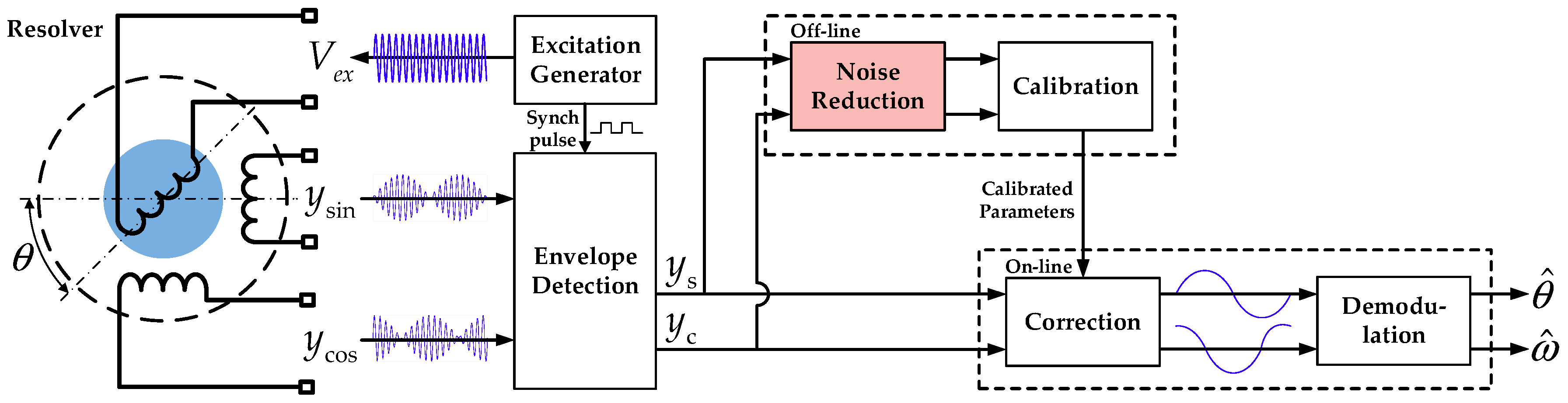
2. Calibration Principle and Problem Formulation of Resolver
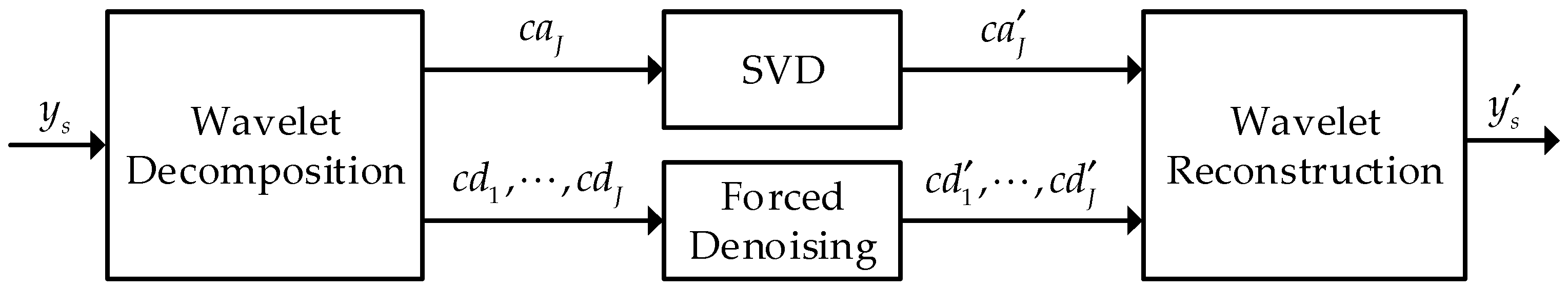
3. Design of DWT-SVD Based Filter
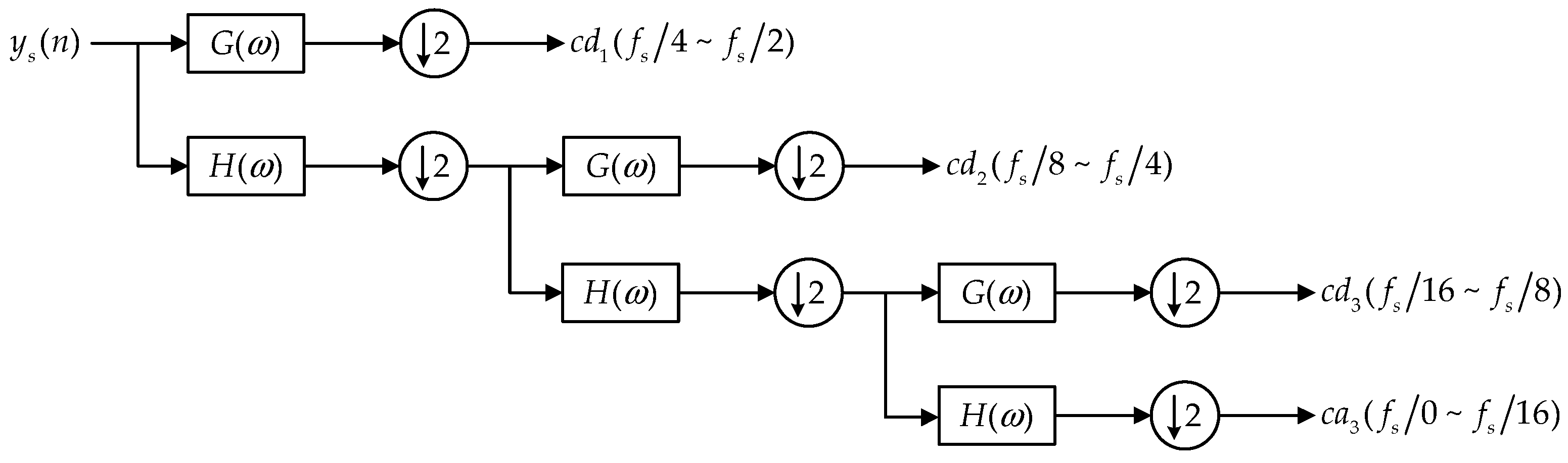
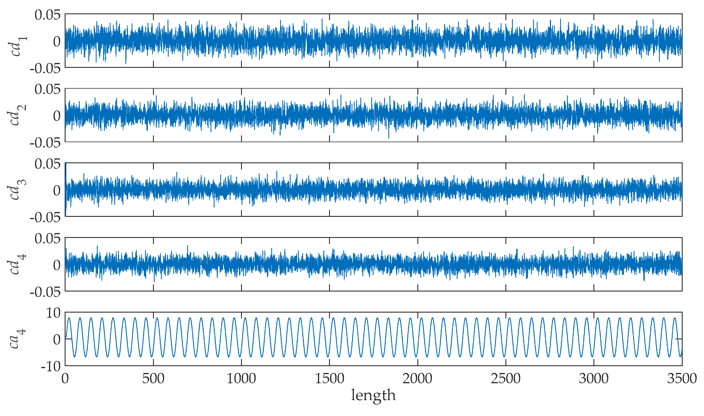
3.1. Signal Decomposition
3.2. Coefficient Processing
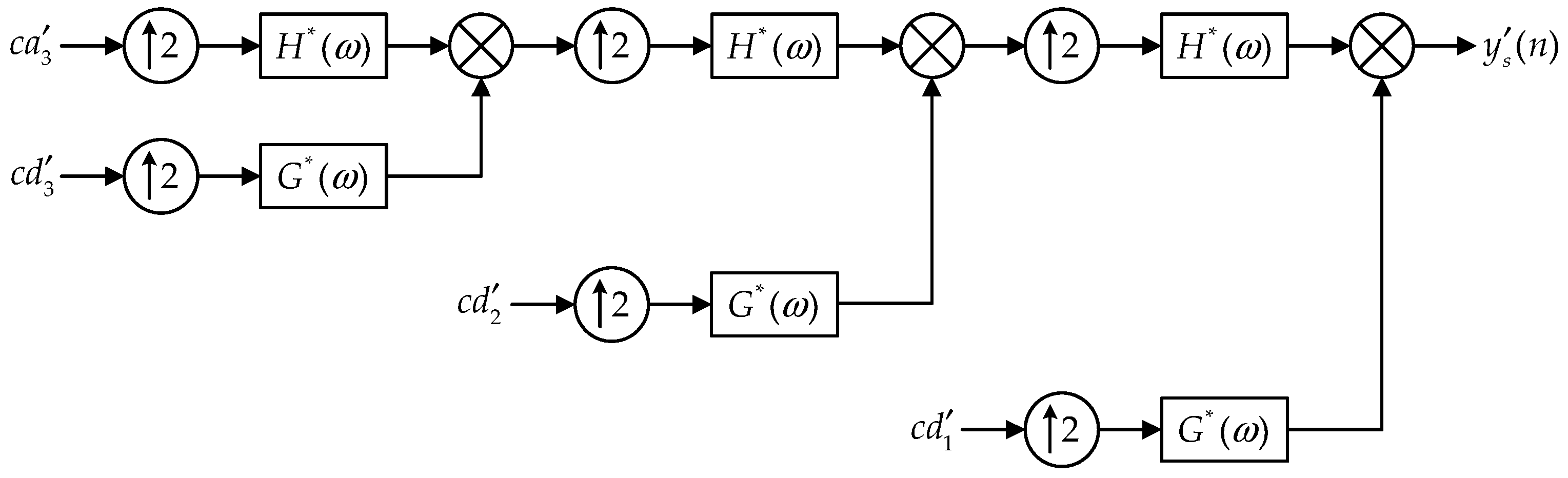
3.3. Signal Reconstruction
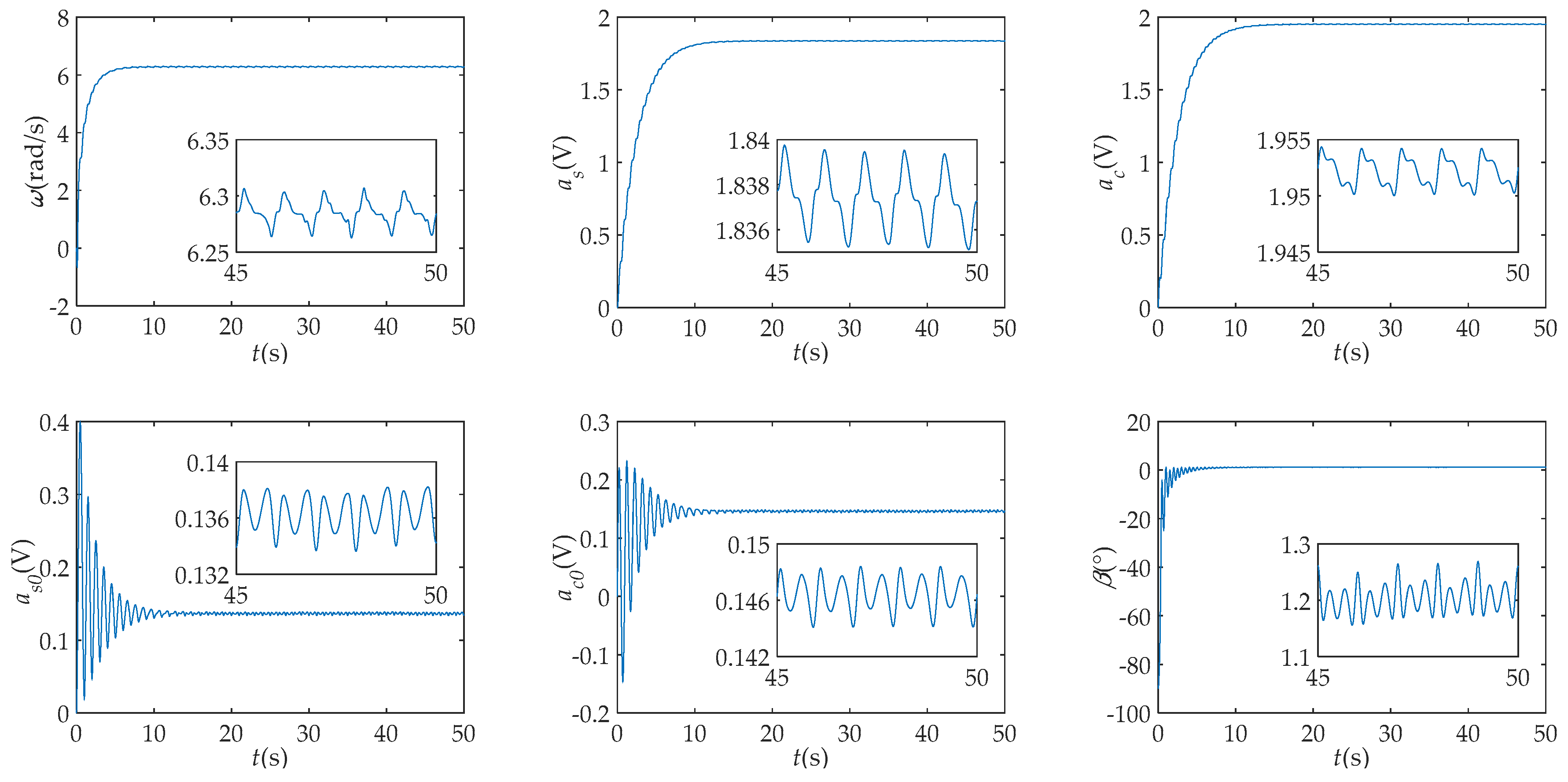
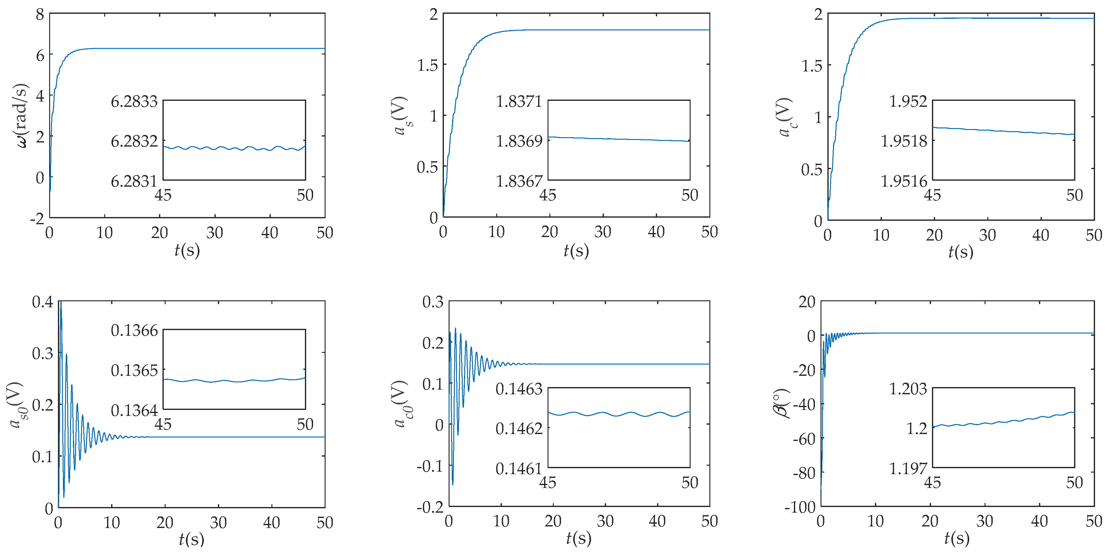
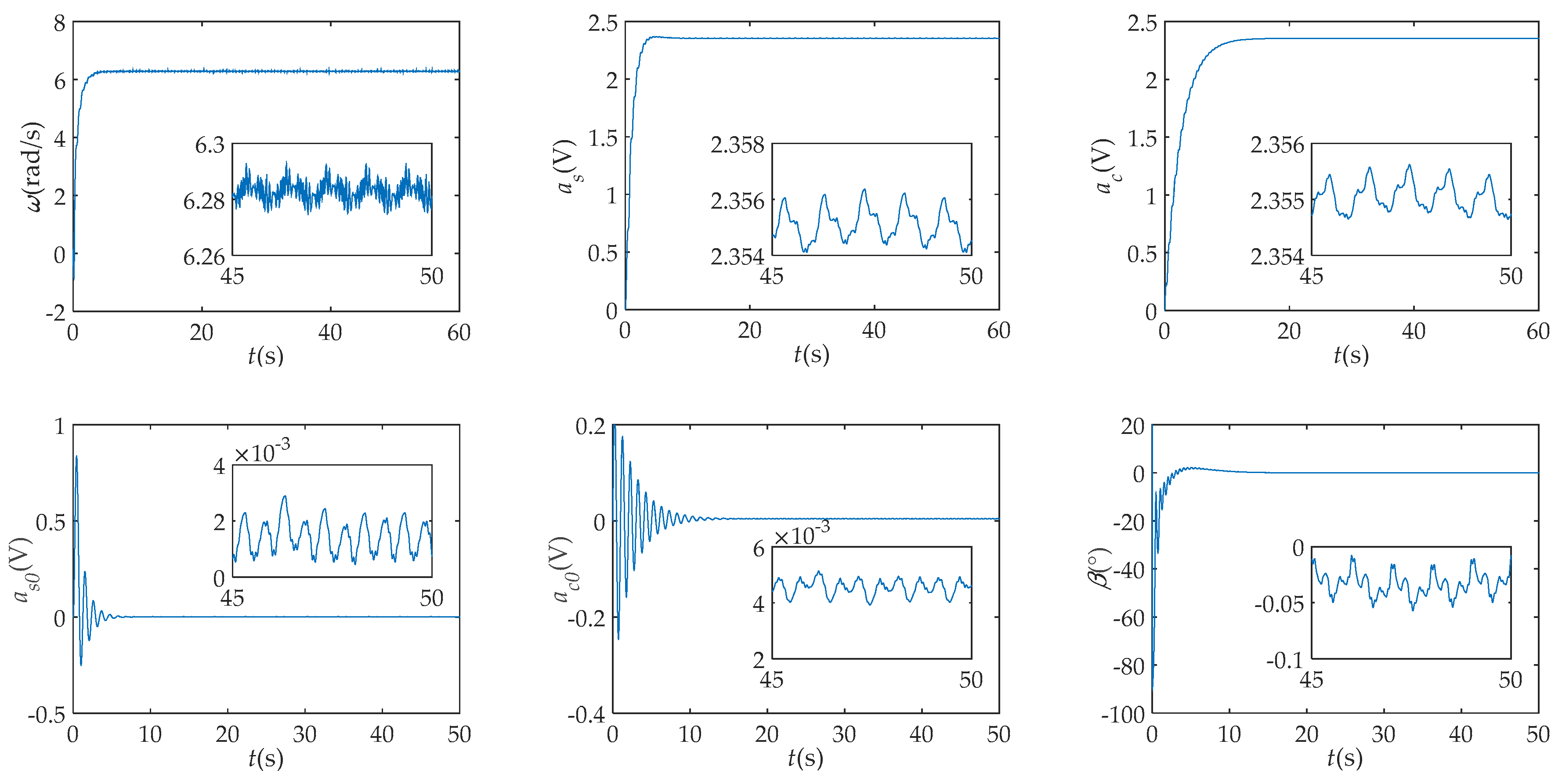
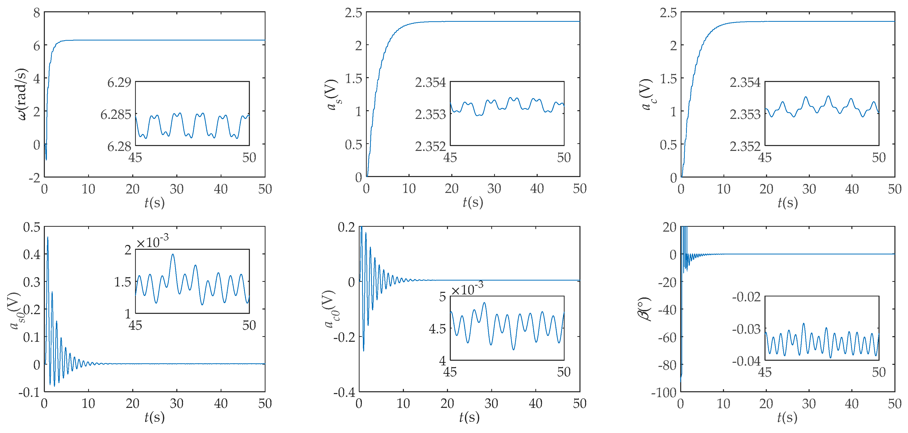
4. Simulation and Experimental Results
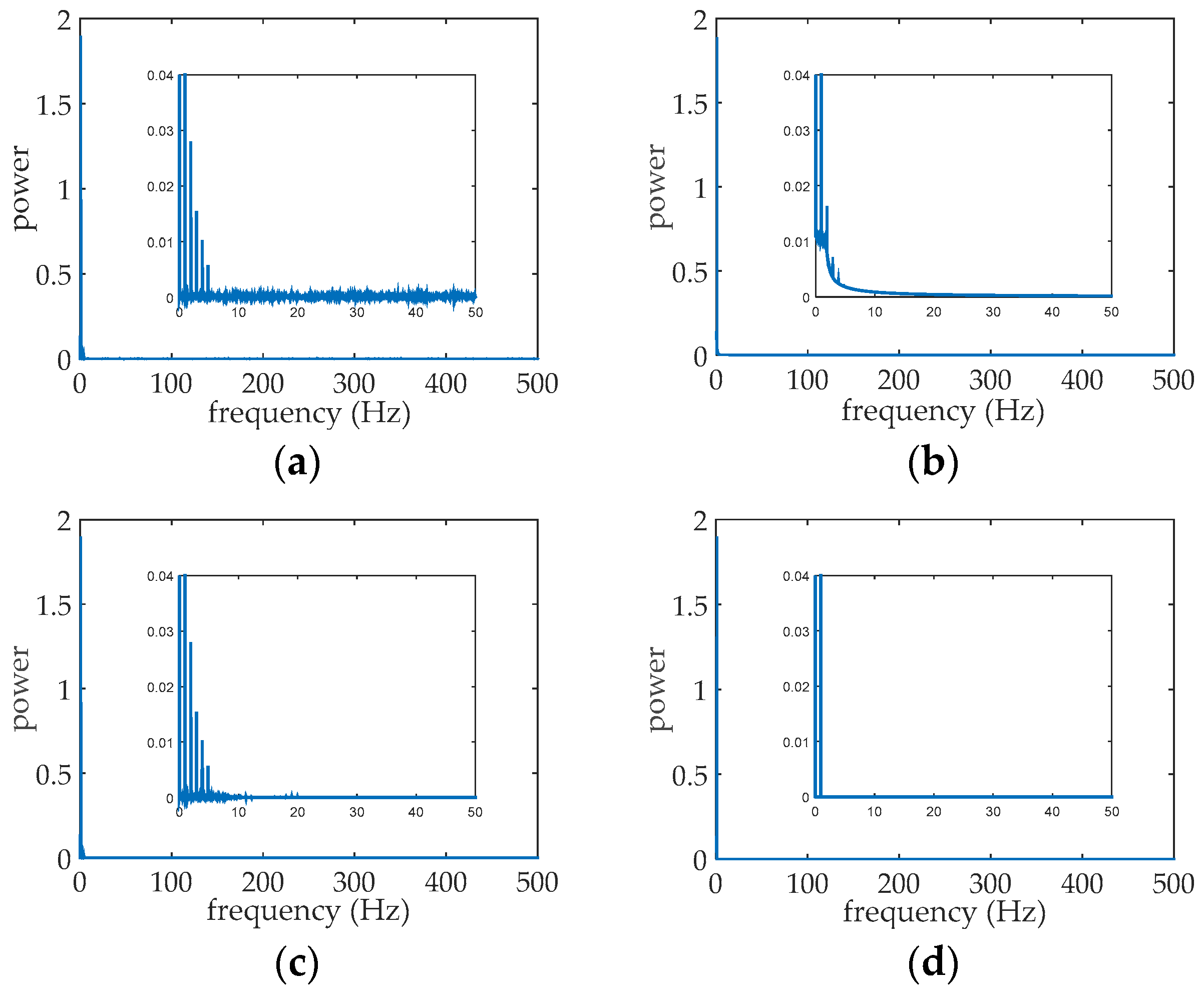
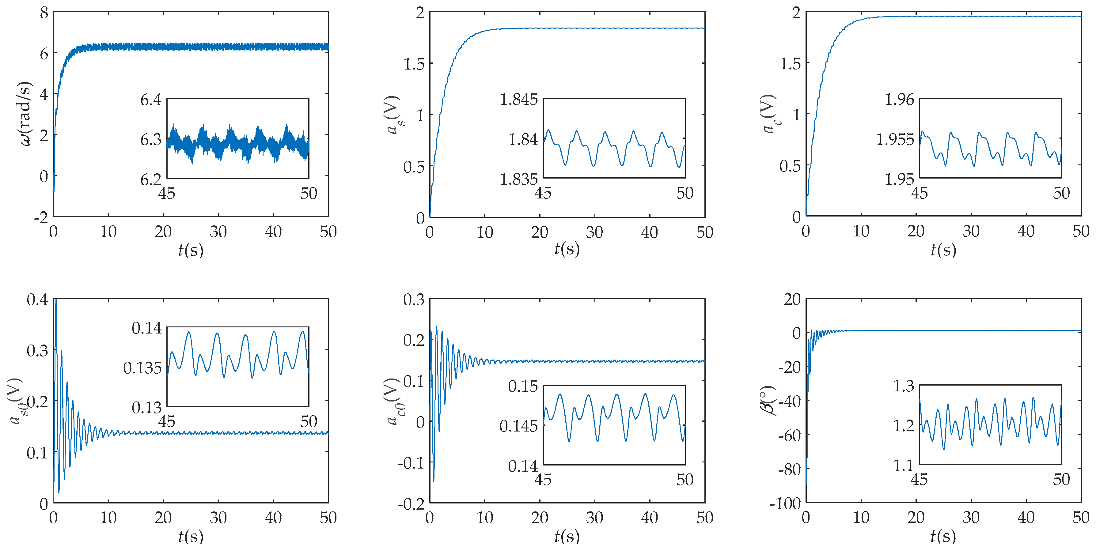
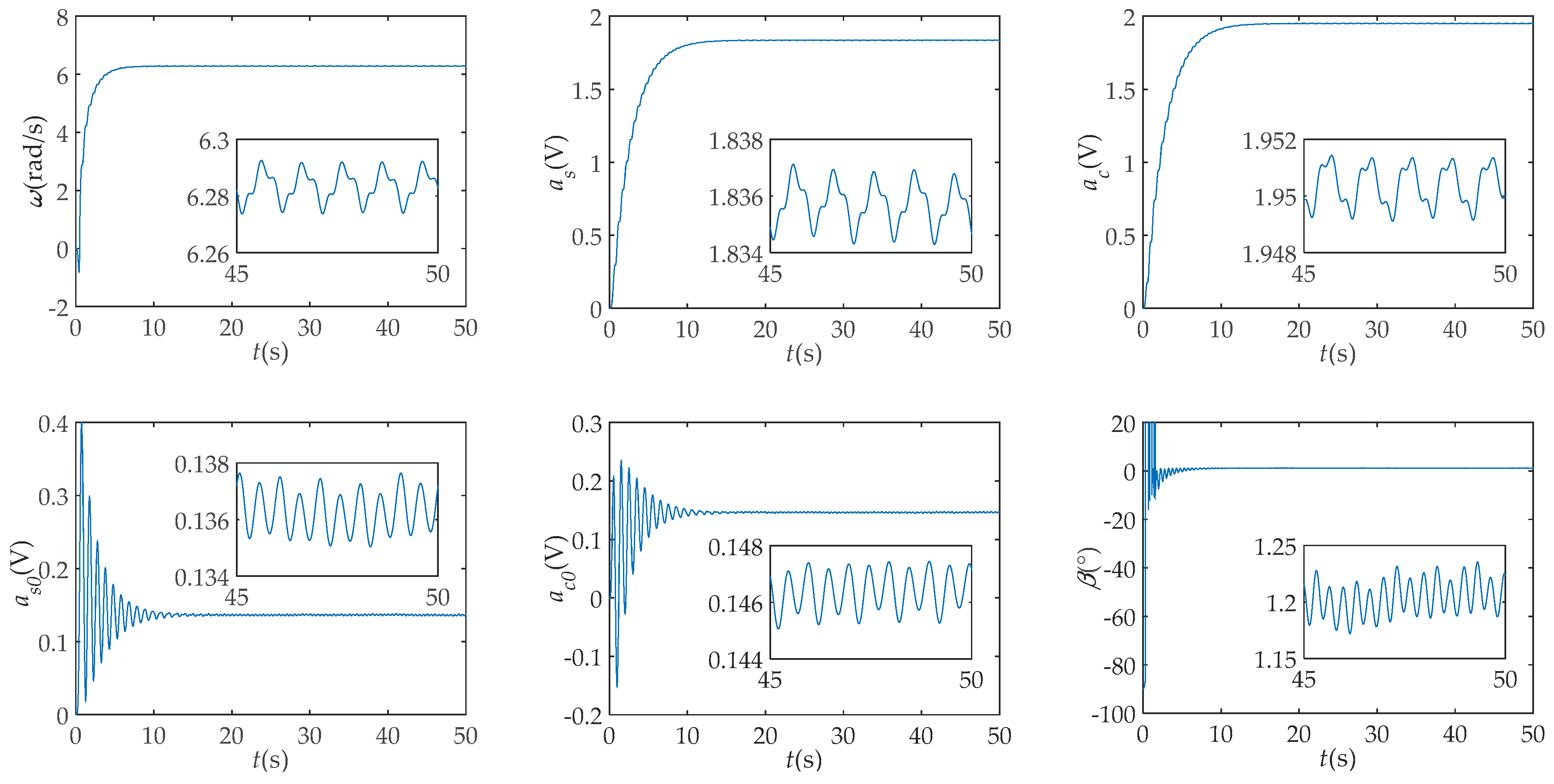
4.1. Simulation Results
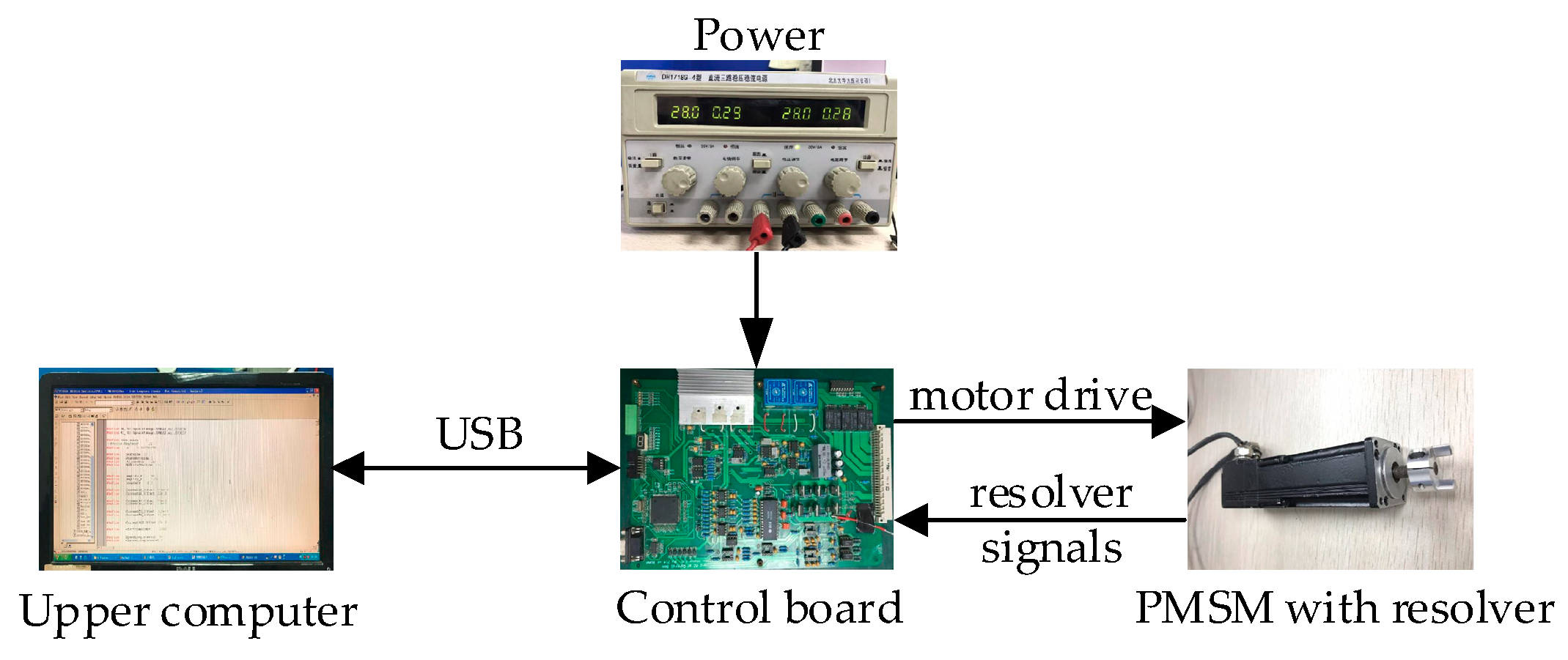
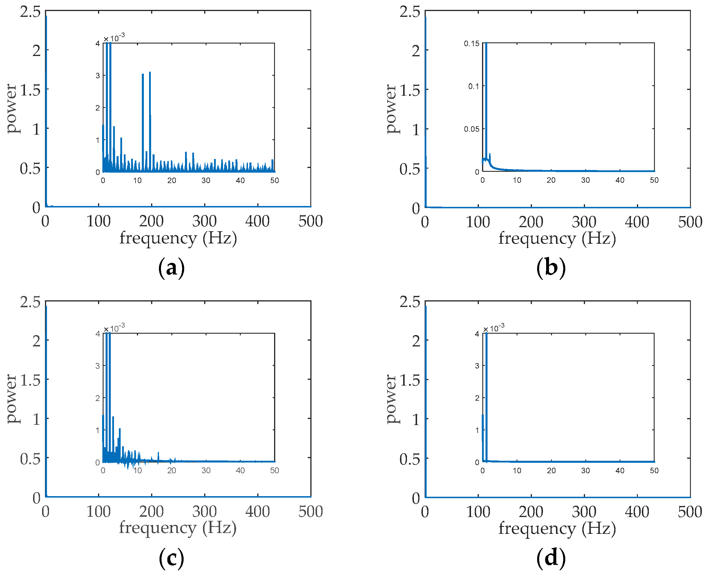
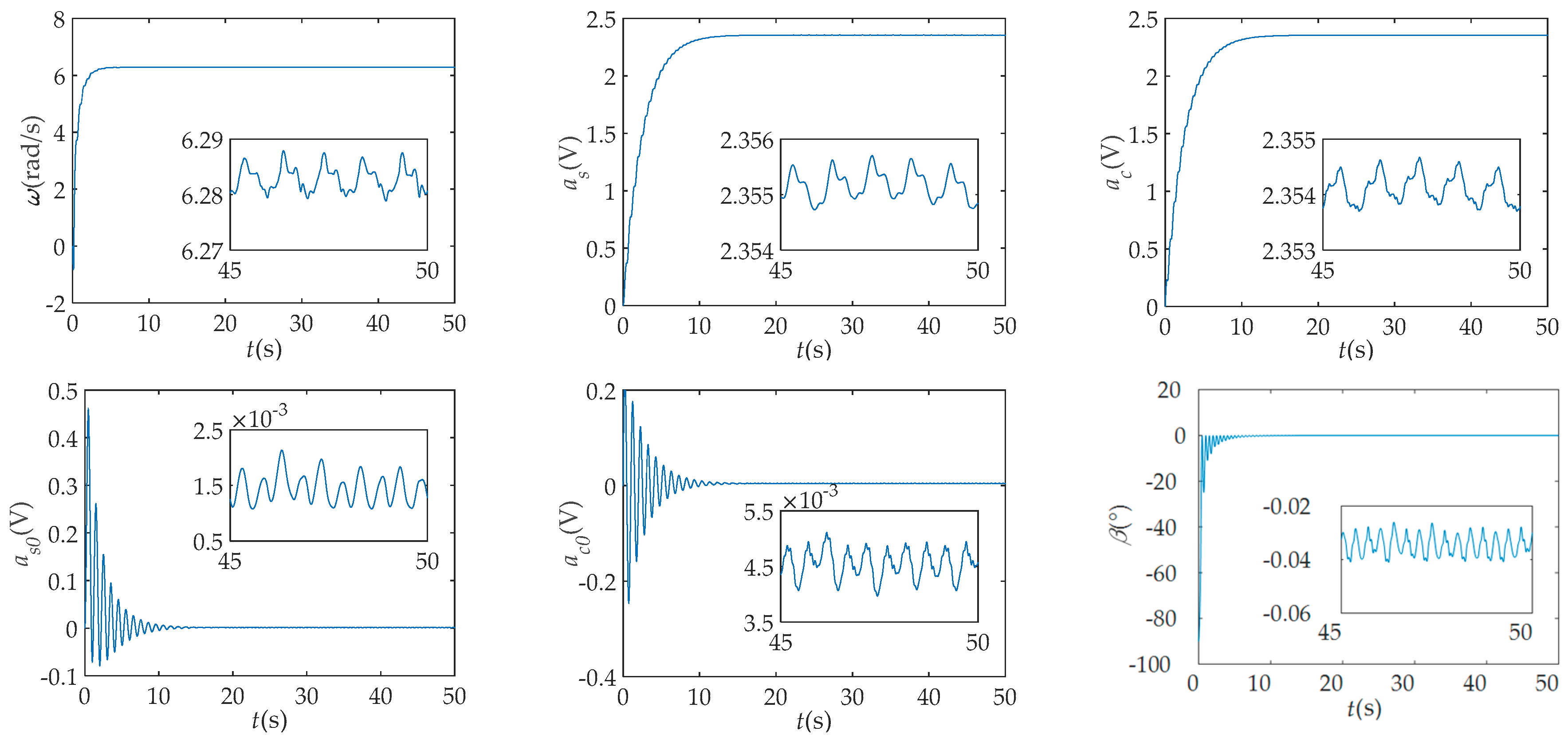
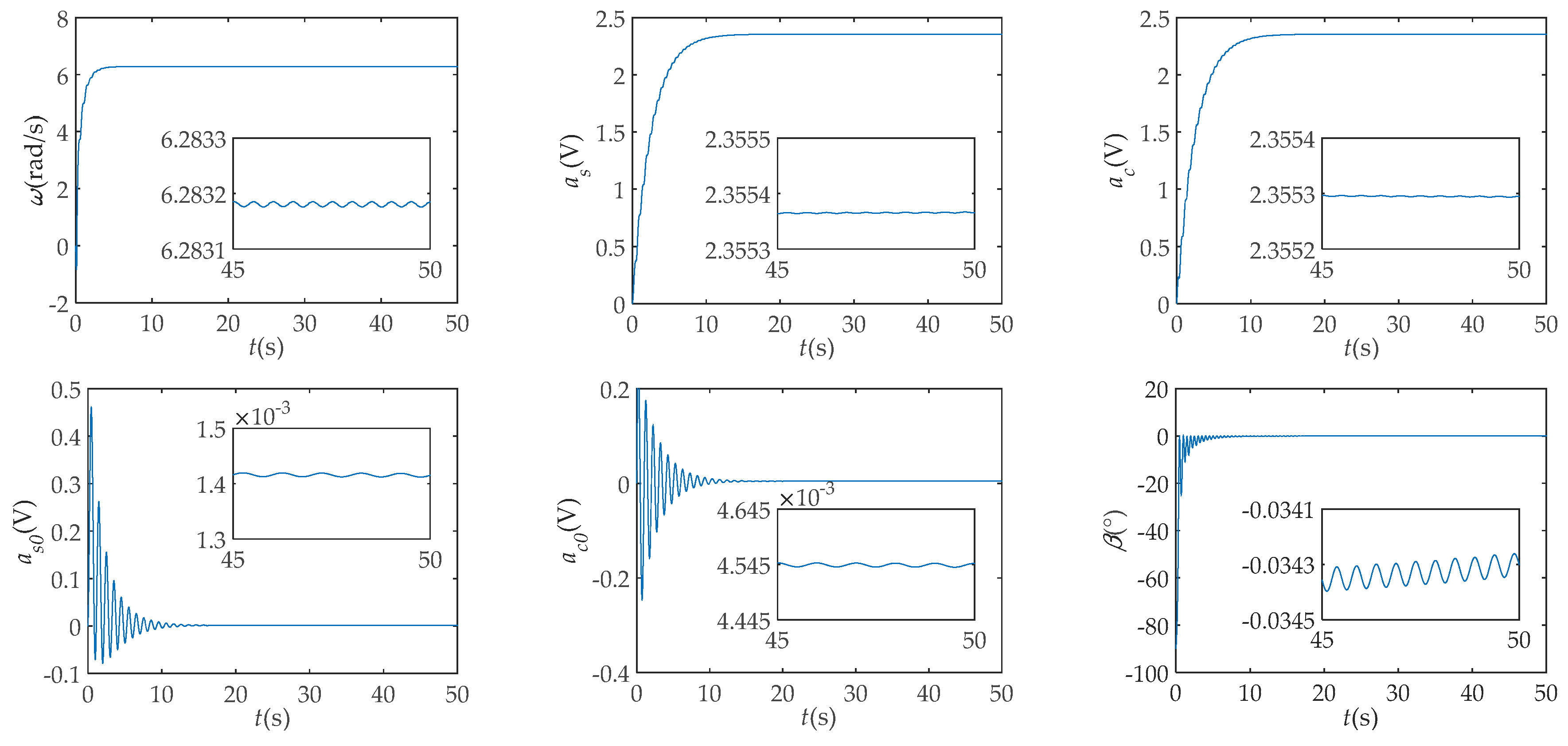
4.2. Experimental Results
5. Conclusions
Author Contributions
Funding
Conflicts of Interest
References
- Alipour-Sarabi, R.; Nasiri-Gheidari, Z.; Tootoonchian, F.; Oraee, H. Performance analysis of concentrated wound-rotor resolver for its applications in high pole number permanent magnet motors. IEEE Trans. Ind. Electron. 2017, 17, 7877–7885. [Google Scholar] [CrossRef]
- Liu, H.; Wu, Z. Demodulation of angular position and velocity from resolver signals via Chebyshev filter-based type III phase locked loop. Electronics 2018, 7, 354. [Google Scholar] [CrossRef]
- Hanselman, D.C. Resolver signal requirements for high accuracy resolver-to-digital conversion. IEEE Trans. Ind. Electron. 1991, 37, 556–561. [Google Scholar] [CrossRef]
- Tan, K.K.; Zhou, H.X.; Lee, T.H. New interpolation method for quadrature encoder signals. IEEE Trans. Instrum. Meas. 2002, 51, 1073–1079. [Google Scholar] [CrossRef]
- Heydemann, P.L.M. Determination and correction of quadrature fringe measurement errors in interferometers. Appl. Opt. 1981, 20, 3382–3384. [Google Scholar] [CrossRef] [PubMed]
- Balemi, S. Automatic calibration of sinusoidal encoder signals. In Proceedings of the 16th Triennial World Congress, Prague, Czech Republic, 3–8 July 2005; pp. 1189–1195. [Google Scholar]
- Hoang, H.V.; Jeon, W.J. Signal compensation and extraction of high resolution position for sinusoidal magnetic encoders. In Proceedings of the International Conference on Control, Automation and Systems, Seoul, Korea, 17–20 October 2007; pp. 1368–1373. [Google Scholar]
- Hoseinnezhad, R.; Bab-Hadiashar, A.; Harding, P. Calibration of resolver sensors in electromechanical braking systems: A modified recursive weighted least-squares approach. IEEE Trans. Ind. Electron. 2007, 54, 1052–1060. [Google Scholar] [CrossRef]
- Zhang, J.; Wu, Z. Automatic calibration of resolver signals via state observers. Meas. Sci. Technol. 2014, 25, 095008. [Google Scholar] [CrossRef]
- Wu, Z.; Li, Y. High-accuracy automatic of resolver signals via two-step gradient estimators. IEEE Sens. J. 2018, 18, 2883–2891. [Google Scholar] [CrossRef]
- Gao, Z.; Zhou, B.; Hou, B.; Li, C.; Wei, Q.; Zhang, R. Self-calibration of angular position sensors by signal flow networks. Sensors 2018, 18, 2513. [Google Scholar] [CrossRef]
- Lara, J.; Chandra, A. Position error compensation in quadrature analog magnetic encoders through an iterative optimization algorithm. In Proceedings of the Industrial Electronics Society IECON 2014—40th Annual Conference of the IEEE, Dallas, TX, USA, 29 October–1 November 2014; pp. 3043–3048. [Google Scholar]
- Wang, H.; Shang, J.; Li, Y.; Xu, Y. The finite element analysis and parameter optimization of the axial flux variable-reluctance resolver with short pitch distributed winding. Int. J. Appl. Electromagn. Mech. 2014, 45, 441–447. [Google Scholar] [CrossRef]
- Kaul, S.K.; Tickoo, A.K.; Koul, R.; Kumar, N. Improving the accuracy of low-cost resolver-based encoders using harmonic analysis. Nucl. Instrum. Methods Phys. Res. 2007, 586, 345–355. [Google Scholar] [CrossRef]
- Faber, J. Self-calibration and noise reduction of resolver sensor in servo drive application. In Proceedings of the 2012 Elektro of the IEEE, Rajeck Teplice, Slovakia, 21–22 May 2012; pp. 174–178. [Google Scholar]
- Sarma, S.; Venkateswaralu, A. Systematic error cancellations and fault detection of resolver angular sensors using a DSP based system. Mechatronics 2009, 19, 1303–1312. [Google Scholar] [CrossRef]
- Zhu, M.; Wang, J.; Ding, L.; Zhu, Y. A Software based robust resolver-to-digital conversion method in designed in frequency domain. In Proceedings of the 2011 International Symposium on Computer Science and Society, Kota Kinabalu, Malaysia, 16–17 July 2011; pp. 244–247. [Google Scholar]
- Minaee, S.; Abdolrashidi, A.A. Highly accurate palmprint recognition using statistical and wavelet features. In Proceedings of the 2015 IEEE Signal Processing and Signal Processing Education Workshop, Salt Lake City, UT, USA, 9–12 August 2015. [Google Scholar]
- Huang, Z.; Li, W.; Wang, J.; Zhang, T. Face recognition based on pixel-level and feature-level fusion of the top-level’s wavelet sub-bands. Inf. Fusion 2015, 22, 95–104. [Google Scholar] [CrossRef]
- Minaee, S.; Abdolrashidi, A. On The power of joint wavelet-DCT features for multispectral palmprint recognition. In Proceedings of the 2015 49th Asilomar Conference on Signals, Systems and Computer, Pacific Grove, CA, USA, 8–11 November 2015; pp. 1593–1597. [Google Scholar]
- Xu, X.; Luo, M.; Tan, Z.; Pei, R. Echo signal extraction method of laser radar based on improved singular value decomposition and wavelet threshold denoising. Infrared Phys. Technol. 2018, 92, 327–335. [Google Scholar] [CrossRef]
- Xu, J.; Zhang, L.; Zuo, W.; Zhang, D.; Feng, X. Patch group based nonlocal self-similarity prior learning for image denoising. In Proceedings of the 2015 IEEE International Conference on Computer Vision, Santiago, Chile, 7–13 December 2015; pp. 244–252. [Google Scholar]
- Zhang, K.; Zuo, W.; Zhang, L. FFDNet: Toward a fast and flexible solution for CNN based image denoising. IEEE Trans. Image Process. 2018, 27, 4608–4622. [Google Scholar] [CrossRef]
- Guo, Q.; Zhang, C.; Zhang, Y.; Liu, H. An efficient SVD-based method for image denoising. IEEE Trans. Circuits Syst. Video Technol. 2016, 26, 868–880. [Google Scholar] [CrossRef]
- Zhao, X.; Ye, B.; Chen, T. The relationship between non-zero singular values and frequencies and its application to signal decomposition. Acta Electron. Sin. 2017, 45, 2008–2018. [Google Scholar]
- Paul, J.S.; Reddy, M.R.; Kumar, V.J. A transform domain SVD filter for suppression of muscle noise artefacts in exercise ECG’s. IEEE Trans. Biomed. Eng. 2000, 47, 654–663. [Google Scholar] [CrossRef] [PubMed]
- Bhatnagar, G.; Raman, B. A new robust reference watermarking scheme based on DWT-SVD. Comput. Stand. Interfaces 2009, 31, 1002–1013. [Google Scholar] [CrossRef]
- Kallel, F.; Hamida, A.B. A new adaptive gamma correction based algorithm using DWT-SVD for non-contrast CT image enhancement. IEEE Trans. Nanobiosci. 2017, 16, 666–675. [Google Scholar] [CrossRef]
- Kumar, M.; Vaish, A. An efficient encryption-then-compression technique for encrypted images using SVD. Digit. Signal Prog. 2017, 60, 81–89. [Google Scholar] [CrossRef]
- Jiang, Y.; Tang, B.; Qin, Y.; Liu, W. Feature extraction method of wind turbine based on adaptive Morlet wavelet and SVD. Renew. Energy 2011, 36, 2146–2153. [Google Scholar] [CrossRef]


| Order | 2 | 3 | 4 | 5 |
|---|---|---|---|---|
| (V) | 0.0255 | 0.0130 | 0.0078 | 0.0032 |
| (V) | 0.0243 | 0.0128 | 0.0082 | 0.0025 |
| Number | 1 | 2 | 3 | 4 | 5 |
|---|---|---|---|---|---|
| Value | 6896.7 | 6893.6 | 1026.7 | 95.2 | 95.1 |
| Parameters | |||||||
|---|---|---|---|---|---|---|---|
| Preset values | 6.283185 | 1.83700 | 1.95200 | 0.13650 | 0.14520 | 1.2000 | |
| Calibrated directly | Estimates | 6.285769 | 1.83893 | 1.95372 | 0.13643 | 0.14632 | 1.2019 |
| STD | 1.20 × 10⁻² | 1.25 × 10⁻³ | 1.26 × 10⁻³ | 1.63 × 10⁻³ | 1.63 × 10⁻³ | 3.02 × 10⁻² | |
| After the Butterworth filter | Estimates | 6.283505 | 1.83577 | 1.95035 | 0.13644 | 0.14631 | 1.2017 |
| STD | 5.20 × 10⁻³ | 7.32 × 10⁻⁴ | 7.00 × 10⁻⁴ | 7.54 × 10⁻⁴ | 6.95 × 10⁻⁴ | 1.48 × 10⁻² | |
| After the DWT | Estimates | 6.283640 | 1.83741 | 1.95210 | 0.13644 | 0.14632 | 1.2019 |
| STD | 1.01 × 10⁻² | 1.22 × 10⁻³ | 1.23 × 10⁻³ | 1.25 × 10⁻³ | 1.18 × 10⁻³ | 2.55 × 10⁻² | |
| After the designed filter | Estimates | 6.283179 | 1.83691 | 1.95187 | 0.13648 | 0.14623 | 1.2002 |
| STD | 2.49 × 10⁻⁶ | 1.11 × 10⁻⁵ | 2.28 × 10⁻⁵ | 4.59 × 10⁻⁶ | 3.44 × 10⁻⁶ | 4.23 × 10⁻⁴ | |
| PMSM | Resolver | ||
|---|---|---|---|
| Pole pairs | 2 | Pole pairs | 1 |
| Rated voltage | 110 V(AC) | Input voltage | 5 V ± 0.2 V (AC) |
| Rated speed | 3000 r/min | Input frequency | 10 kHz |
| Torque constant | 0.15 Nm/A | Output voltage | >2 V |
| Phase resistance | 8 Ω | Transformer ratio | 0.5 ± 5% |
| Phase inductance | 10 mH | Electrical error | |
| Number | 1 | 2 | 3 | 4 | 5 | 6 | 7 |
|---|---|---|---|---|---|---|---|
| value | 9418.9 | 9410.4 | 19.8 | 19.7 | 11.7 | 9.3 | 9.2 |
| Parameters | |||||||
|---|---|---|---|---|---|---|---|
| Calibrated directly | Estimates | 6.28288 | 2.3551 | 2.3550 | 1.446 × 10⁻³ | 4.548 × 10⁻³ | −0.03450 |
| STD | 2.88 × 10⁻³ | 2.54 × 10⁻⁴ | 2.56 × 10⁻⁴ | 2.85 × 10⁻⁴ | 2.86 × 10⁻⁴ | 3.99 × 10⁻³ | |
| After the Butterworth filter | Estimates | 6.28304 | 2.3532 | 2.3532 | 1.445 × 10⁻³ | 4.545 × 10⁻³ | −0.03462 |
| STD | 1.80 × 10⁻³ | 1.54 × 10⁻⁴ | 1.57 × 10⁻⁴ | 1.70 × 10⁻⁴ | 1.66 × 10⁻⁴ | 2.44 × 10⁻³ | |
| After the DWT | Estimates | 6.28299 | 2.3552 | 2.3541 | 1.447 × 10⁻³ | 4.547 × 10⁻³ | −0.03448 |
| STD | 2.19 × 10⁻³ | 2.48 × 10⁻⁴ | 2.53 × 10⁻⁴ | 2.56 × 10⁻⁴ | 2.57 × 10⁻⁴ | 3.83 × 10⁻³ | |
| After the designed filter | Estimates | 6.28318 | 2.3553 | 2.3532 | 1.416 × 10⁻³ | 4.544 × 10⁻³ | −0.03436 |
| STD | 3.30 × 10⁻⁶ | 7.99 × 10⁻⁶ | 1.07 × 10⁻⁷ | 2.48 × 10⁻⁶ | 2.54 × 10⁻⁶ | 4.16 × 10⁻⁵ | |
© 2019 by the authors. Licensee MDPI, Basel, Switzerland. This article is an open access article distributed under the terms and conditions of the Creative Commons Attribution (CC BY) license (http://creativecommons.org/licenses/by/4.0/).
Share and Cite
Guo, M.; Wu, Z. Noise Reduction for High-Accuracy Automatic Calibration of Resolver Signals via DWT-SVD Based Filter. Electronics 2019, 8, 516. https://doi.org/10.3390/electronics8050516
Guo M, Wu Z. Noise Reduction for High-Accuracy Automatic Calibration of Resolver Signals via DWT-SVD Based Filter. Electronics. 2019; 8(5):516. https://doi.org/10.3390/electronics8050516
Chicago/Turabian StyleGuo, Meishan, and Zhong Wu. 2019. "Noise Reduction for High-Accuracy Automatic Calibration of Resolver Signals via DWT-SVD Based Filter" Electronics 8, no. 5: 516. https://doi.org/10.3390/electronics8050516
APA StyleGuo, M., & Wu, Z. (2019). Noise Reduction for High-Accuracy Automatic Calibration of Resolver Signals via DWT-SVD Based Filter. Electronics, 8(5), 516. https://doi.org/10.3390/electronics8050516