1. Introduction
With the increasing complexity of the electromagnetic environment, the existing radar signal recognition techniques cannot meet the needs of practical application. At the same time, recognition of radar signals arriving at the receiving device has become a key technique in the field of electronic countermeasures [
1]. In a real electromagnetic environment, there are usually many radars detecting transmitter signals to steal information from transmitters. After radar signals are detected by the receiving device, they should be separated and recognized in time, and the types, quantity, and threat level of threat radars should then be analyzed with other pulse parameters, so as to take effective measures to jam radar to protect transmitter information from being stolen.
Considering the strategic value of radar signal recognition, many scholars devote themselves to signal recognition. In the early study of radar signal recognition, it is generally accepted and widely used to achieve parameter matching by studying pulse description word (PDW), thus recognizing several common modulation types of radar signals into corresponding categories [
2]. The non-Gaussian, non-stationarity, and non-linearity of radar signals limit time domain or frequency domain analysis [
3]. As a bilinear time-frequency distribution, the Wigner–Ville Distribution (WVD) has excellent characteristics, such as high resolution, energy concentration, and time-frequency edge characteristics [
4]. However, Pachori points out that WVD is prone to cross-term interference when dealing with multi-component signals [
5]. In [
6], Lunden combines WVD, Choi–Williams distribution (CWD), and a classification system to achieve accurate pulse compression waveform recognition. When the signal-to-noise ratio (SNR) is 6 dB, the recognition rate can reach 98% on the premise that each signal takes 1.65 s. It cannot be ignored that the increasing variety of signal types makes it difficult to extract features manually, which makes it difficult to represent the characteristics of the recognized signals comprehensively [
7]. Deep learning (DL) applies an unsupervised or semi-supervised feature learning algorithm to achieve automatic feature extraction [
8]. As important branches of DL, convolutional neural networks (CNNs) and deep belief networks (DBNs) have achieved good results in the field of image recognition by virtue of their own advantages [
9]. In [
10], a CNN-based system for recognizing radar signal was proposed to achieve a recognition rate up to 90% at an SNR of −6 dB by training a large number of samples. However, due to the deep layers and complicated structure of the CNN, the entire recognition process takes a long time. Compared with a CNN, the structure of a DBN more easily obtains basic features of a signal. The application of a DBN to recognize a radar signal may achieve better performance.
Due to the increasingly complex electromagnetic environment in the battlefields of electronic warfare, intercepted radar signals often have many modulations. The adaptive separation of radar emitter signals and the accurate recognition of their modulations have become the most important tasks. At present, the most widely used and practical method of signal separation is blind source separation (BSS), which can accomplish signal separation with little or no prior knowledge. Independent component analysis (ICA) [
11], fast independent component analysis (FastICA) [
12], and sparse component analysis (SCA) [
13] have successively become the mainstream of BSS. However, in the actual battlefield electromagnetic environment, there is only a single receiving device. The above-mentioned multi-channels BSS methods cannot meet those needs. The current popular processing technique is to virtualize a single channel problem into multi-channel BSS, and it then applies prior arts for subsequent processing. EMD can decompose signals into multiple components to construct virtual multi-channels with its adaptability. The biggest challenge is that it is prone to modal aliasing [
14]. An improved algorithm named ensemble empirical mode decomposition (EEMD) is proposed to deal with the disadvantage of EMD. It is worth mentioning that EEMD can only limit modal aliasing to a certain extent and cannot solve the problem fundamentally [
15]. The variational mode decomposition (VMD) explored by Dragomiretskiy is a non-recursive way to decompose signals, which completely solves the drawbacks of EMD and EEMD [
16]. Note that the performance of the VMD is completely dependent on setting the penalty factor and the number of components, which determine the component bandwidth and the degree of decomposition. The group intelligent optimization algorithms is a parameter optimization technique that does not rely on expert experience and can be applied to solve engineering optimization problems. Theoretically, applying a group intelligence algorithm to the parameters of the optimized VMD will achieve the desired effect [
17]. In addition, the common problem of all group intelligent optimization algorithms is that it takes a high amount of time to iteratively search. Signal separation necessarily results in partial loss of the secondary component, especially at low SNR. It makes most classifiers unable to extract representative features when recognizing the secondary component. With the gradual deepening of AlexNet [
18], VGGNet [
19], and GoogleNet [
20], a CNN can alleviate this difficulty to a certain extent with its strong adaptability and automatic feature extraction capabilities. In view of the fact that the increase in the number of layers makes the network unable to effectively train, ResNet adds the connected channel to the network directly, which well solves the problem of degradation of existing network coexistence [
21]. Moreover, it does not introduce additional parameters and computational complexity on the premise of further deepening the layer. However, a CNN faces the challenge of over-extracting features, and it is urgent to choose the most representative features. There are many analytical methods that use matrix decomposition to solve practical problems such as principal component analysis (PCA) [
22], singular value decomposition (SVD) [
23], and linear discriminant analysis (LDA) [
24]. In all of these methods, the original large matrix approximation is decomposed into a low rank form. Note that there can be no negative pixels in the image data, and these dimensionality reduction techniques cannot guarantee non-negativeness of the original data. Furthermore, a CNN has its limitations that cannot be overcome. For example, the training samples required by a CNN are large, and the extracted features do not reflect the nature of the signal [
25,
26,
27]. The combination of multi-classifier and transfer learning can give full play to the advantages of each classifier and overcome the problem of sample loss. The proposed method should obtain better recognition performance in theory.
The main contributions of this paper can be summarized as follows: (1) Regression variational mode decomposition (RVMD) combines support vector regression (SVR) to quickly fit the optimal VMD parameters corresponding to signals while exploring the artificial bee colony (ABC) algorithm to optimize VMD. (2) The technique of regarding VMD as the separator and denoiser is proposed, and DBN is explored as a feature extractor and classifier to speed up recognition while improving the recognition rate of the first component. (3) Aiming at the problem of sample loss in CNN training, the performance of ResNet50 is improved by developing transfer learning, and the effectiveness of the system is further improved by non-negative matrix factorization (NMF). (4) A new fusion network based on DBN and ResNet50 is explored to recognize the secondary component in real time accurately. The proposed system can separate and recognize eight types of radar signals, which are described in context.
The paper is organized as follows.
Section 2 introduces the system model and signal types involved in this paper. The optimal recognition scheme when faced with different numbers of source signals is explored in
Section 3.
Section 4 explains and discusses the experimental results. The conclusions are drawn in
Section 5.
2. System Overview
Considering that our retrieval ability is limited, no mature radar signal separation and recognition technique has been found, so this paper mainly studies the mixing of double signals. As we all know, BPSK, LFM, Costas, Frank code, P1–P4 codes, and T1–T4 codes are the most common modulations of radar emitter signals. Among them, the differences between the four types of polytime codes are more obvious. The main purpose of this paper is to realize the recognition of radar signals with similar performance in various domains, so we selected eight types of radar signals, including BPSK, LFM, Costas, Frank code, and P1–P4 codes. In this section, we show the model of the received signal, the eight types of radar emitter signals considered in this paper, and the structure of the proposed system.
2.1. Signal Model
It is essential to construct a reasonable signal model before conducting experimental verification. Assume that the received signals are polluted by additive white gaussian noise (AWGN) and the amplitude is constant for time. Consider the discrete time model
can be expressed as
where
k is the sample index increasing every
for a sampling
,
is AWGN of power
and mean of 0,
N is the number of the components of the received signals,
A is an invariant constant, and
is the instantaneous phase of the corresponding sub-signal, the analytic signal of the
nth component
. If the received signal is real, the Hilbert transform is used:
where the Hilbert transform of
is given by
where
means the integral taken in the sense of the Cauchy principal value. In this model, when
, the proposed system can recognize the signal’s modulation after denoising directly. Similarly, when
, the modulation mode of each sub-signal needs to be separated first and then recognized. In this paper, only the cases of
are considered for the time being, but the other cases can also be analogized to achieve satisfactory results using the proposed technique.
The eight types of common radar emitter signals considered in this paper are as follows: BPSK, LFM, Costas code, and five polyphase codes (such as Frank and P1–P4 codes).
can be expressed jointly by instantaneous frequency
and the phase offset
as follows:
The eight radar emitter signals mentioned above can be divided into two kinds of pulse compression methods: FM (frequency modulation) and PM (phase modulation), as shown in
Table 1.
In addition, for Frank, P1, and P2 codes, , , whereas i for P3 and P4 codes satisfies .
2.2. System Structure
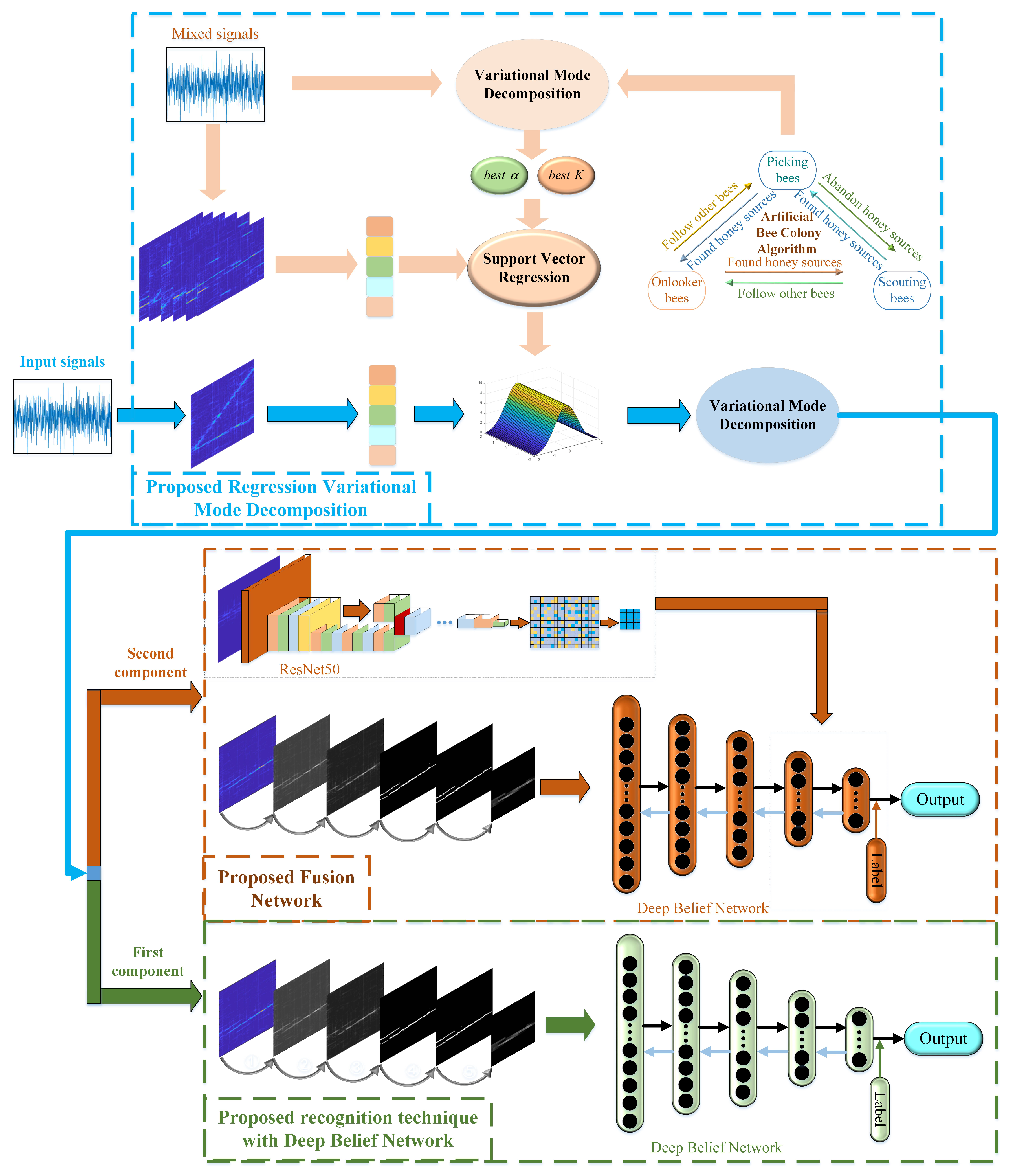
Assume that the number of received signals is known to be two, and the two signals are equal power. Meanwhile, the modulations of the two mixed signals are different. The block diagram of the proposed system that depicts single radar signal recognition, multiple signal separation, and multiple signal recognition of the proposed system is given by
Figure 1. The main objective of this paper is to recognize each sub-signal accurately and in real time when source signals are received. Note that we use the components separated by RVMD to represent the sub-signals. Firstly, when signals are intercepted by the receiving device, the proposed system can quickly establish a fitting relationship between the VMD parameters optimized by an offline ABC algorithm and the Renyi entropy of the received signals by means of SVR. VMD is used to separate the signals and remove the noise of the signals, and the preprocessed time-frequency image of the first component is then sent to DBN for recognition. Next, ResNet50 is combined with the technique of transfer learning and with NMF as the feature extractor of the secondary component. Finally, the secondary component is preprocessed and sent to the fusion network composed of the DBN and the feature extractor.
3. Proposed System
3.1. Single Signal Recognition
3.1.1. Denoising Technique with VMD
The signal intercepted by the receiving device is bound to be polluted by noise. If noise is eliminated to a certain extent before the signal is recognized, the recognition rate can be further improved.
As an emerging signal decomposition technique, VMD is able to separate the components of the signal. VMD is a variable-scale signal processing method with theoretical support to decompose the complex signal into
K component signals [
16]. First, transform the optimization problem to an unconstrained optimization problem, as shown in Equation (
5):
where
is the center frequency,
,
,
. The value of
a ensures the accuracy of the reconstruct signal. The combination of
a and
not only makes
a with limited weight have well convergence, but also makes restrictions keep strict. The variational problem is then solved, and detailed steps are shown in Algorithm 1.
| Algorithm 1 The solution of variational problem. |
| Input:Output: |
| 1: Initialize: , , , |
| 2: Repeat |
| 3: for do |
| 4: Update :
|
| 5: end for |
| 6: for do |
| 7: Update : |
| 8:
|
| 9: end for |
| 10: Dual ascent:
|
| 11: Until convergence: |
| 12:
|
Considering that this technique is suitable for receiving single radar signals, the penalty factor and the component number K of VMD can be set to 2000 and 2 by default. Finally, the principal sub-signal separated by the VMD is taken out for subsequent processing.
3.1.2. Recognition Technique with DBN
Because the traditional manual extraction of image features is limited in practice, it is urgent to explore an effective method for extracting features that can improve the reliability of radar signal recognition. A DBN can extract the essential features of samples more quickly and accurately. It combines the advantages of unsupervised learning and supervised learning and has a good recognition ability for high-dimensional data. The application of a DBN in radar signal recognition requires preprocessing images of the signals and training the DBN model with a training set.
A. Image preprocessing
In order to recognize the modulation mode of the radar signal, it is necessary to extract features with high discrimination. However, there will be a high amount of overlap in the time and frequency domains, which makes the extracted signal’s features unsatisfactory. Therefore, the signal will be converted to a time-frequency domain before extracting the features. CWD is a time-frequency transformation that can effectively suppress cross-terms [
6]:
where
is the kernel function,
is the controllable factor,
is the time delay, and
k and
represent time and frequency components of time-frequency analysis, respectively. As a parameter to weigh cross-terms and resolution, the control factor satisfies
. If time and frequency are expressed as
x- and
y-axes respectively, the time-frequency analysis can be regarded as two-dimensional images that are shown in
Figure 2.
In addition, a fast CWD based on fast Fourier transform (FFT) is presented in [
7]. The number of sampling points is recommended to be a power of two, such as 128, 256, 512, etc. In this paper, 1024 × 1024 points are selected. If the sequence length is less than 1024, it is complemented by zero. Furthermore, a reasonable preprocessing method for images can effectively eliminate noise and redundant information while effectively enhancing signal information.
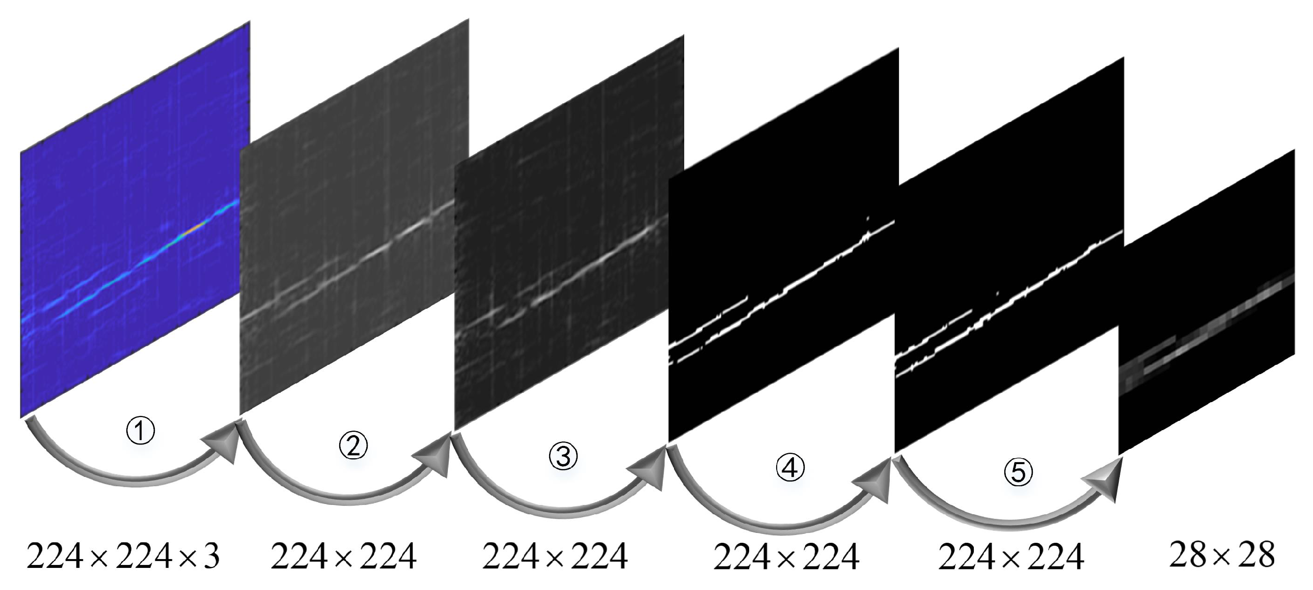
Figure 3 shows the specific scheme of image preprocessing used in this subsection.
Step 1: The gray image is carried out to reduce the computational complexity of the subsequent image:
Step 2: The gray values of the gray image are normalized to reduce the imbalance between data:
Step 3: Binarize the resulting image to save storage space:
Step 4: Implement close operation for improving the recognition rate, which makes the contour components of the image smooth and further reduces noise:
where
,
, and
denote the gray values of the three channels of the color image,
is the preset threshold, ⊕ denotes an expansion operation,
denotes an expansion corrosion operation,
is the structural element, and
represents the image after close operation on
.
B. DBN Training
DBN consists of a multi-layer unsupervised restricted Boltzmann machine (RBM) network and a supervised back propagation (BP) network [
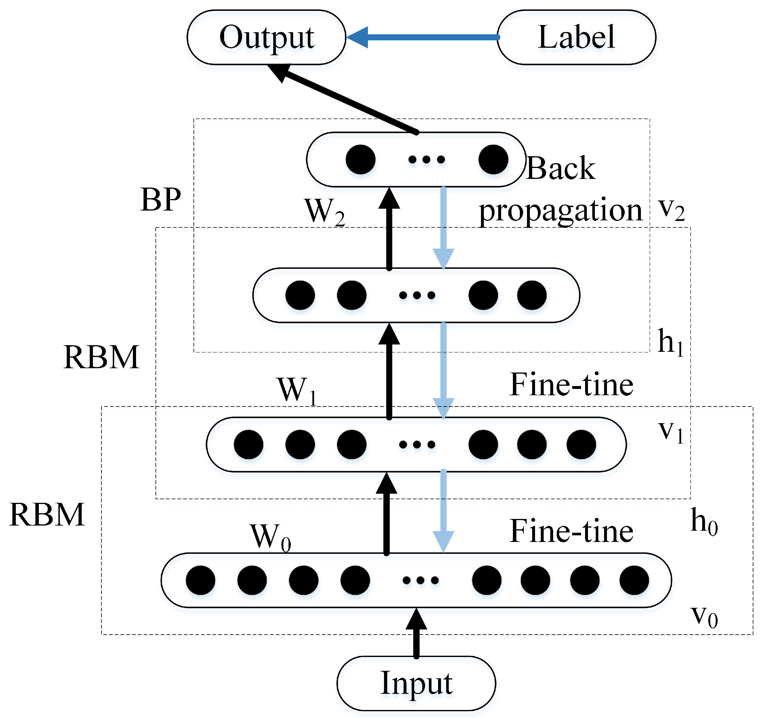
27], which trains a hidden layer to capture the correlation of high-order data in the visual layer. The RBM acts as a data compressor when the number of neurons in the hidden layer is less than that in the visual layer. The typical architecture of the DBN is shown in
Figure 4. Because the image composition of the radar signal is not complex, the number of RBMs is set to 3, and the DBN corresponding to the number of neurons in each hidden layer is 200. This can fully meet the needs of radar signals recognition.
The preprocessed image of the radar signal is transformed into one-dimensional information
x and input into the RBM. The DBN trains the RBM in each layer by the training layer, as shown by the dark arrow. There is a weight
W between any two connected neurons in the RBM to indicate their connection strength. Each neuron has its own bias coefficients
b (for visual neurons) and
c (for hidden neurons) to express its own weight. In this way, the following functions can be used to represent the energy of an RBM:
where
and
are neurons in the visual and hidden layers, and
and
represent the number of visual and hidden neurons, respectively. There is a certain probability that the hidden layer neuron
will be activated:
Because of the bidirectional connections between neurons, the visual neurons can also be activated by the hidden neurons.
where
is a Sigmoid function, which can also be set to other functions. The RBM is trained iteratively by the contrast divergence algorithm, and the weight is updated continuously. After several training sessions, the hidden layer can not only accurately display the characteristics of the visual layer, but also restore the visual layer. Because the output of the visible layer of the upper RBM is used as the input of the hidden layer of the lower RBM, it is necessary to train the RBM of the upper layer thoroughly before training the RBM of the current layer, and and this process must continue to the last layer of the RBM.
However, each layer of the RBM network can only guarantee that the weight of its own layer is optimal for its eigenvector mapping, not for the whole DBN. Therefore, a BP network can fine-tune the DBN network by transmitting error information from top to bottom to each layer of the RBM, as shown by the light arrow [
28]. In the last layer of the DBN, the BP network receives the output eigenvector of the RBM as its input eigenvector. Then we train the classifier of DBN according to the input of BP network.
3.2. Regression VMD with Double Signals
Theoretically, a DBN can achieve ideal results in recognizing the modulation mode of a radar signal. However, in an actual electromagnetic environment, it is common for multiple signals to arrive at the receiver at the same time. At present, there is no effective technique that can recognize the modulation mode of each sub-signal in the received signals directly. Therefore, the effective separation of received signals is the first priority.
Similarly, when double signals are intercepted by the receiving device, it is separated by VMD. After intensive study, it is found that the penalty parameter in the VMD algorithm also has a greater impact on the decomposition results. The smaller is, the wider the bandwidth of each IMF component is, and, on the contrary, the smaller the bandwidth of the component signal is. Because the actual signal to be analyzed is complex and changeable, it is usually difficult to determine the two influencing parameters of K and . Selecting the appropriate combination of parameters is key to the separation of multiple signals using the VMD algorithm. Since this paper only considers the mixing of double signals, regardless of where K goes, only the first two components will be selected for analysis.
3.2.1. ABC Algorithm for VMD
As a better global swarm intelligence optimization algorithm, the ABC algorithm is proposed to select the best combination of VMD parameters [
29]. Because there are two parameters to be optimized, the solution space of the problem is two-dimensional. Assuming that the number of employer bees and onlooker bees is
, which is equal to the number of honey sources, the ABC algorithm will search in the two-dimensional search space.
In addition, when using the ABC algorithm to search the influence parameters of the VMD algorithm, it is necessary to determine a fitness function. The fitness value is calculated once every time the particle updates its position. The fitness value is updated by comparing the fitness value of the new particle. Envelope entropy can quantify the fluctuation and flatness of the signal envelope and reflect the sparse characteristics of the original signal. Envelope entropy of
can be expressed as
where
is the normalized form of envelope signal obtained by Hilbert demodulation of
. When radar multiple signals are separated by VMD, the signals with smaller IMF component noise have stronger sparsity and smaller envelope entropy. The minimum of all IMF components of a food source is calculated as the local minimum entropy value, but the component is only the local optimal component. In order to find the global optimal component, the local minimum entropy can be used as a fitness value in the optimization process, and the reciprocal of the local minimum entropy can be used as the ultimate optimization objective. Algorithm 2 shows the steps of VMD parameter optimization.
| Algorithm 2 ABC algorithm for VMD. |
| Input:: envelope signal of Output: best K, best |
| 1: Initialize: : the initial solutions of population |
| 2: : the initial fitness value |
| 3: |
| 4: repeat |
| 5: for each employed bee
|
| Apply greedy selection process
|
| 6: for each onlooker bee |
| 7: Select a solution depending on |
| Apply greedy selection process |
| 8: If exist an abandoned solution |
| 9: Then replace it with a new solution
|
| Memorize the best solution so far |
| 10: |
| 11: until |
where
,
,
, and
is a random number in
. The correlation between the original honey source location
and the random honey source location
affects the new honey source location
,
is the fitness value of
,
R is a random number in
, and
and
are upper and lower bounds of the
jth dimension, respectively.
3.2.2. Adaptive Signal Separation
Although it is easier to obtain the global optimal solution by optimizing the parameters of VMD with the ABC algorithm, its search speed is slow. This is a fatal problem of swarm intelligence optimization algorithm, which needs to be solved urgently. As a statistical analysis method to study the relationship between two groups of variables, regression can build a bridge between them quickly. Thus, the technique named RVMD is proposed to realize rapid adaptive separation of radar multiple signals.
SVR is a powerful machine learning method, which is of great significance to the construction of data-driven non-linear empirical process model. SVR has the unique ability to find the best compromise between model complexity and learning ability according to limited sample information and to finally transform the problem into a quadratic programming problem. At the same time, introducing the idea of a kernel function can solve the problems of a small sample, non-linearity, and high dimension ideally. It has been extended to solve the problem of non-linear regression estimation. Assume the sample training set
, where input
and output
. SVR can find a relatively flat function to approximate the relationship between input and output of the sample set through training samples and can also give an accurate output to the new input [
30]. The regression function
can be expressed as
where
and
b denote weight vector and threshold, respectively,
denotes the inner product of vectors, and
denotes the high dimensional feature space that is nonlinearly mapped from the input space. According to the structural risk minimization principle,
is equivalent to solving the following optimization problems:
where
and
denote slack variables that measure the cost of error pertaining to up-side and down-side of the regression respectively,
C denotes the penalty factor,
denotes the true value of
,
denotes the accuracy of approximation, and
. By introducing the Lagrange function, Equation (
29) can be solved by means of their dual problems
where
denotes the kernel function.
can be expressed as
where
and
denote the relaxation variable. Moreover, selecting suitable model variables is a necessary step for regression analysis using SVR.
Renyi entropy is a method of quantitatively describing signal information, which can reflect the amount and complexity of signal information [
31]. Therefore, Renyi entropy is proposed as the input variable of support vector regression. Renyi entropy of an image can be expressed as
Obviously, the stability condition of Equation (
29) is
Since the even Renyi entropy of multi-component signals and non-linear FM signals is easily affected by cross-terms, this paper mainly considers the odd order with better stability. Meanwhile, the higher the order, the smaller the Renyi entropy of the time-frequency distribution. With the increasing of , the Renyi entropy of all signals will converge to the same value gradually. Hence, the Renyi entropy of the third, fifth, seventh, ninth, and eleventh order with higher discrimination is regarded as an independent variable. Renyi entropy and the parameters of VMD are defined as input variables and output variables, respectively. In addition, since the current research has not provided an appropriate method of selecting the kernel function and parameters in theory, only by experimental means can they be selected. In this paper, the cross validation method is used, and the kernel function of the SVR model is chosen as an RBF kernel function. Furthermore, an appropriate training set is selected to establish an ideal support vector machine model, which lays a solid foundation for the follow-up empirical prediction.
On the basis of the ABC algorithm and SVR, the relationships between the features of signals and the optimal VMD parameters can be established by pre-offline training. When the multiple signals arrive at the receiving device, the ideal VMD parameters can be obtained quickly by extracting only a few features of the signal. However, there are some unpredictable problems when using the DBN to recognize the modulation modes of sub-signals: the recognition rate of the principal sub-signal is very ideal, but the recognition rate will decrease sharply as the component becomes weaker. Therefore, how to recognize each sub-signal accurately is an urgent problem.
3.3. Fusion Network with Double Signal
Because the advantage of a DBN is that the extracted features can reflect the essence of the signal, it can be used to separate the principal component to achieve an ideal recognition rate. However, the incomplete separation of weak sub-signals causes some basic information to be hidden, and a DBN is no longer suitable for it. In order to realize rapid accurate recognition of each sub-signal, the fusion network is proposed. The DBN is combined with ResNet50 to extract signal features more comprehensively. In view of the shortcomings of ResNet50, which lacks a large number of training samples, the transferable ResNet50 is explored.
3.3.1. Transferable ResNet50
As a network with outstanding performance in image classification, ResNet50 can extract image details more comprehensively. Meanwhile, in order to solve the gradient dispersion problem of a deep network training a CNN, a fast connection method of deep ResNet is proposed. On the premise of guaranteeing data fluency between networks, the problem of under-fitting caused by the disappearance of gradient is avoided, which deepens the network level and effectively improves the expressive ability of the model.
Assuming that
is the network output corresponding to the input sample
x in the neural network [
21], it can fit any function and be consistent with the input dimension. Let
be a residual function. It can be verified that the objective of fitting is equivalent to that of fitting
. On this basis, the original function
can be expressed as
. The output of the network can be obtained by adding the output of
x after several residual layers to the original
x. The output is defined as
where
z is the output vector of the network, and
is a residual mapping to be learned. If the dimensions of
x and
are different, the calculation between input and output can be realized by linear projection
on shortcut connection.
In order to simplify the symbols, the deviation term is omitted in the output formula. The residual module must contain at least two convolution layers. If there is only one convolution layer, the residual module is a linear layer, which loses the advantage of residual learning. All in all, ResNet50 realizes data superposition between input and output by a shortcut connection without increasing the number of network parameters and computational complexity.
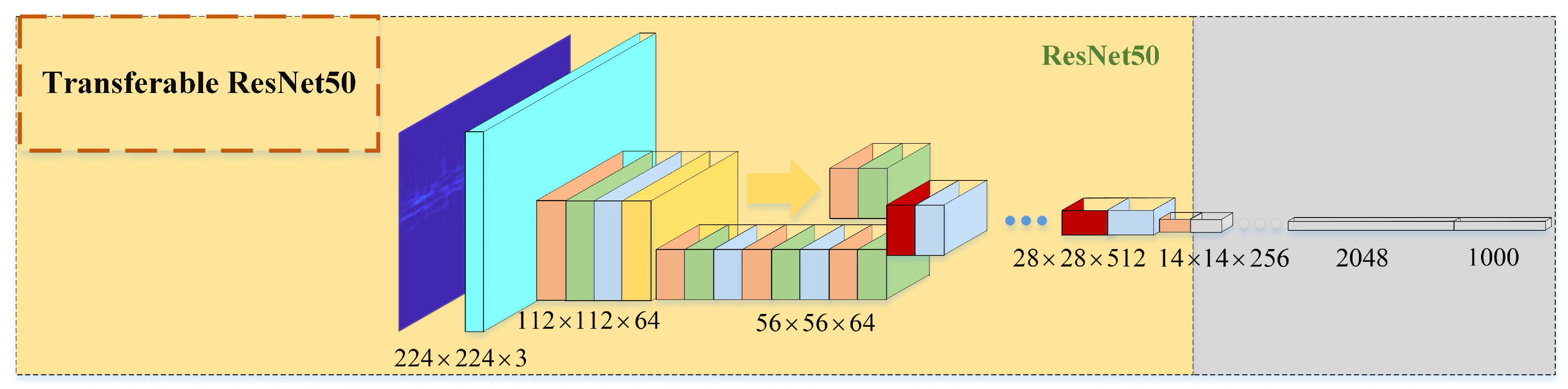
In this paper, ResNet50 is selected as a feature extractor for the secondary component besides the DBN, considering that the recognition rate is obviously improved while the minimum running time is sacrificed. However, ResNet50 needs a high amount of training data, but in reality there is a lack of radar signal samples. Inspired by the transfer learning, the proposed technique utilizes the pre-training ResNet50 model provided by Matconvnet. On the premise of fixing the original parameters of Resnet50, the res4a_branch2a layer, which can extract the details of the image, is set as the output layer. The network structure of Transferable Resnet50 is given by
Figure 5. The CWD images of the secondary component is then fed into the module to extract the detailed features of the radar signal.
3.3.2. Feature Dimension Reduction and Network Fusion
In order to solve the problem of a high dimension and a large amount of computation of features extracted by the ResNet50 module, the NMF technique is used to reduce the dimension of features to improve the recognition rate [
32].
Given a non-negative
matrix
and a preset positive integer
, NMF finds matrix
and matrix
, which satisfy
. The common way to find
and
is to minimize the Euclid distance between
and
.
The row vectors of are features after dimension reduction. After dimensionality reduction, features extracted by Resnet50 and DBN are fused to form final features, which are fed into the BP network of the DBN to recognize the modulation mode of the secondary sub-signal.
4. Simulation Results and Discussion
In this section, the performance of the proposed system is analyzed by presenting simulation results. In AWGN channels, separation and recognition performance are measured as a function of the SNR. SNR can be expressed as
, where
and
are the variances of the original signal and noise, respectively. The sampling points are set to 1024. In practice, in order to save the cost of the project and reduce the sampling requirements of the analog-to-digital converter on the premise of guaranteeing the receiving quality, the received high frequency radar signals are usually down-converted. Therefore, we define the sampling frequency of the radar signals as 256 MHZ in the experiments. In addition, in order to reduce the errors caused by unpredictable factors, we obtain the average value of the 200 times result. The parameter settings of eight radar signals are shown in
Table 2.
4.1. Performance with Single Signal Recognition
In this section, the training set and test set for single signal recognition are generated randomly according to
Table 2. The SNR of the signal will be increased from −6 dB to 6 dB at an interval of 2 dB. It is worth mentioning that there are 600 samples for each signal type per SNR, 500 samples for the training set, and the remaining samples for the testing set.
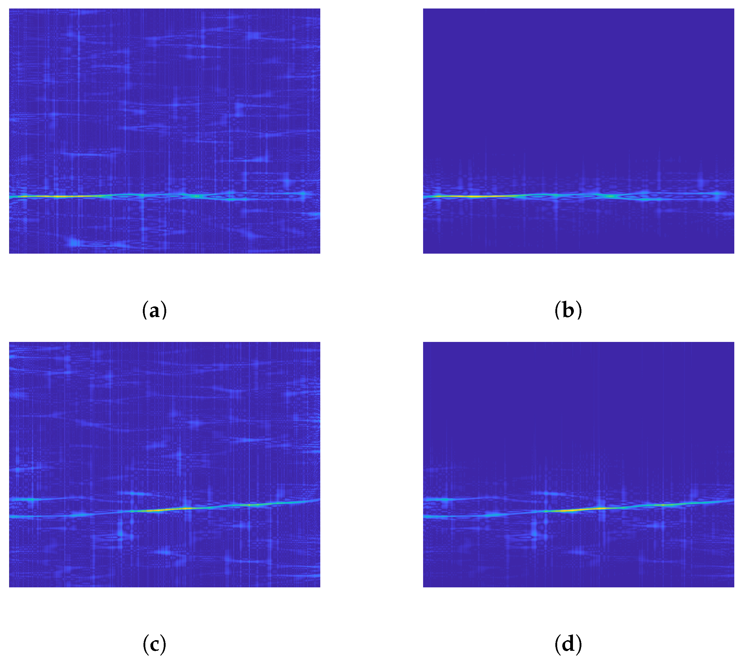
Figure 6 shows the effect of applying the proposed denoising technique before recognizing BPSK and Frank code when the SNR is −6 dB. Obviously, the image noise points after VMD denoising are significantly reduced, which is due to the ability of VMD to quickly find the critical point of each component when facing a simple noisy signal.
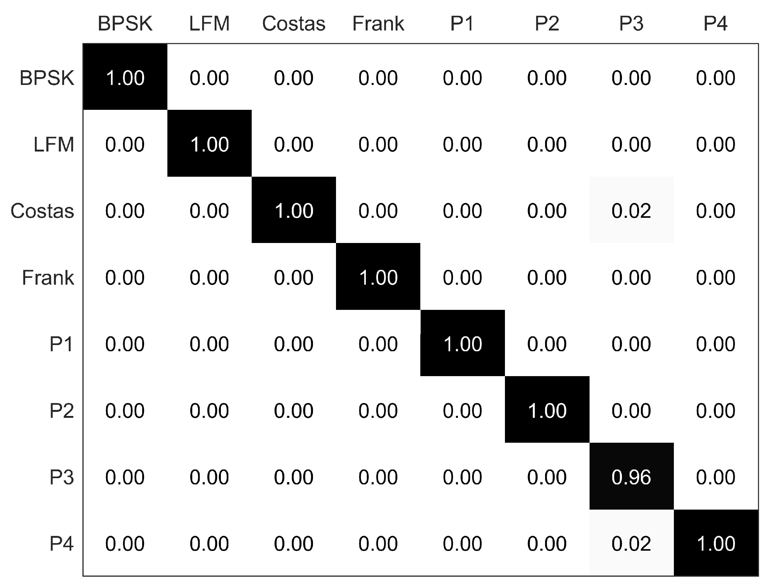
The confusion matrix of eight radar emitter signals at the SNR of 0 dB is presented in
Figure 7. The overall recognition rate can reach 99.50%. It is noteworthy that there are some errors in the P3 codes; they are misjudged as Costas and P4 codes. The high recognition rate achieved by the DBN benefits from the superior self-training and feature extraction capabilities of the DBN.
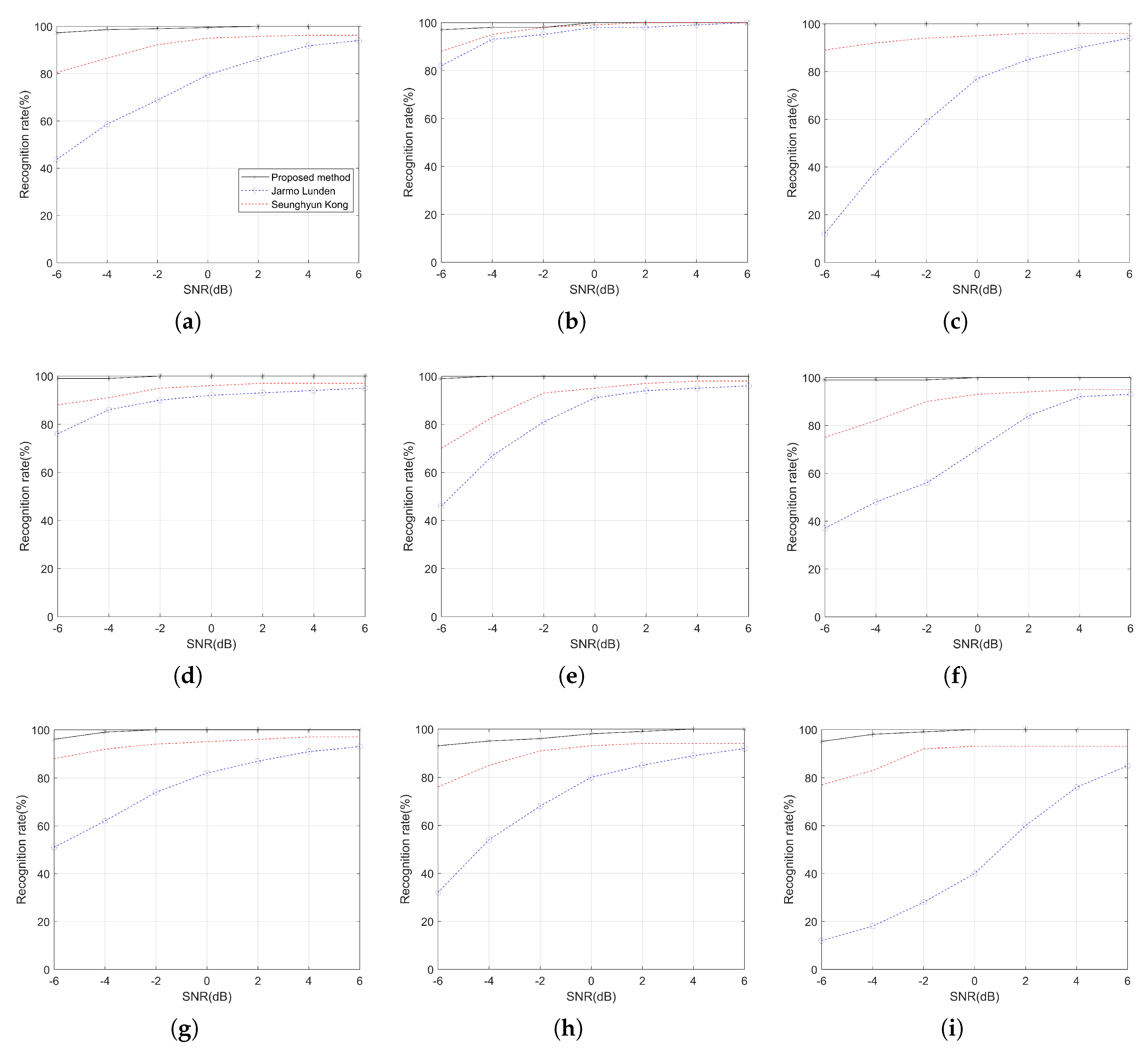
The recognition rates overall, and each signal using the DBN at different SNRs, are shown in
Figure 8. The same experimental conditions are set to achieve a comparison of the results with Lunden’s [
6] and Kong’s [
10] systems, which are systems for radar signal recognition. The solid line represents the proposed signal recognition system applying DBN, and the dotted lines represent Lunden’s and Kong’s systems. Obviously, the recognition rates of the three systems have something in common; that is, the higher the SNR, the higher the recognition rate. Compared with Kong’s system, the recognition rate of each signal under a low SNR is significantly improved on the premise that the recognition rate of the system is more ideal under any noise condition. However, the recognition rates of BPSK and Costas are slightly higher than that of the Lunden’s system. The recognition rates of the other seven signals in the proposed system are much higher than that of Lunden’s system. Undoubtedly, the DBN is able to automatically extract features, and the extracted features are closer to the nature of the signal, thus achieving a higher recognition rate than existing systems.
Of course, the advantages of the proposed method are not limited to a high recognition rate. Lunden introduces features such as second-order statistics into the recognition system and sacrifices the effectiveness of the system in order to improve the recognition rate. Meanwhile, Kong’s system requires a large number of training samples as a basis, and the network structure is more complicated than the DBN. Compared to the 1.65 s and 1.35 s cost of the two existing systems, the proposed technique shortens the time required to recognize the signal at 0.8 s. This is due to the DBN’s unique self-training advantage when dealing with small samples. In addition, considering the structure of the DBN, the input image size of the DBN is much smaller, and the number of layers is small.
4.2. Separation Performance with RVMD
With the increasing complexity of the electromagnetic environment and the emergence of new institutional radars, multiple signals arrive at the receiving device at the same time in most cases. This section shows the specific performance of the proposed system in establishing a regression relationship and separating signals. It should be noted that this section only considers the case of linear mixing of double signals.
The validation of the regression relationship between the Renyi entropy of the signal and the parameters of VMD is based on randomly choosing two of eight signals as a group. Five samples of each combination form are randomly selected under each SNR as a training set. In order to establish a more comprehensive and accurate relationship between them, the SNR range of each signal is −6 to 6 dB, and the interval is 2 dB. Thirty samples satisfying the requirements of the above SNR environment and training set were randomly selected as the test set to test the regression performance.
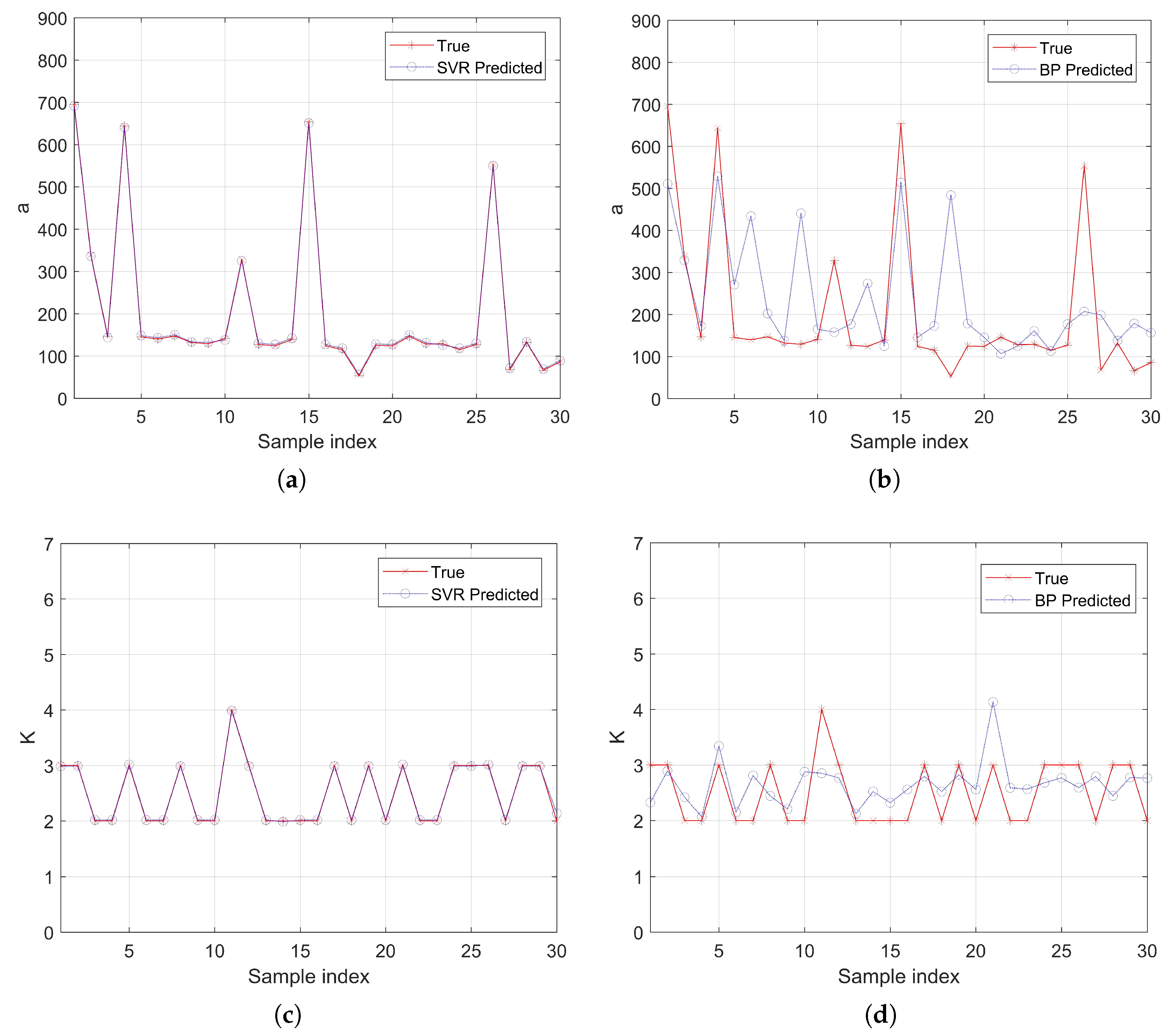
Figure 9 shows the performance of using SVR and BP networks to establish regression relationships, respectively. It is clear from the figures that the VMD parameters corresponding to different signals are not fixed. Compared with the BP network, SVR can fit
and
K perfectly, except for the slight difference in the 30th sample of
K. In addition, since the values of
K are all integers, they can be rounded. Therefore, the success rate of using SVR to establish the regression relationship between Renyi entropy and VMD parameters can be regarded as 100%. The simulation results are due to the difference of mechanism between the BP network and SVR. SVR solves the problem of over-reliance on learning samples by constructing a regression estimation function, which further enhances the generalization ability of the BP network. In addition, the slow convergence of the BP network can be perfectly overcome by SVR.
After the regression relationship is established, test signals are needed. When the test signals arrive at the receiving equipment, the optimal
and
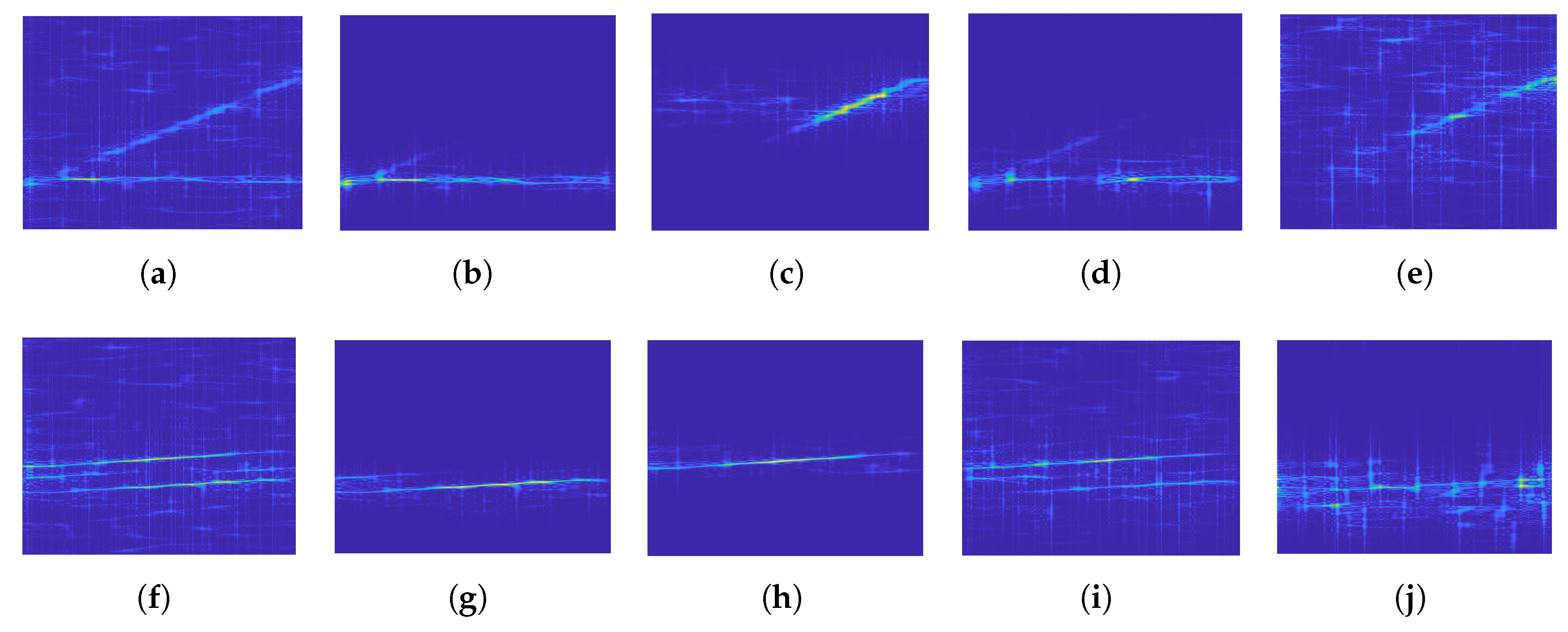
K can be obtained quickly according to the regression relationship. As shown in
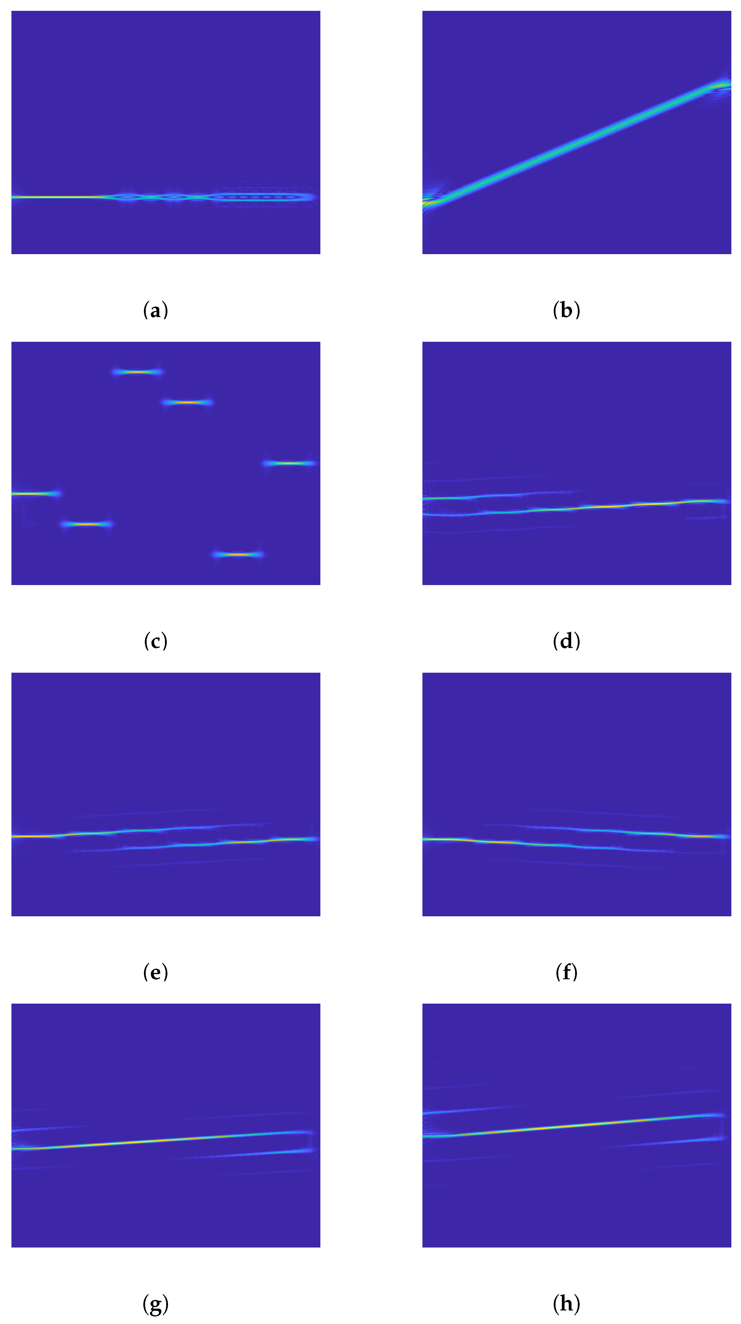
Figure 10, we randomly selected two combinations with an SNR of 0 dB as test signals. From left to right in the sub-graphs are the received multiple signals, the two sub-component signals separated by RVMD and separated by EEMD. Obviously, all the principal sub-signals separated by RVMD remain intact and highly differentiated. For the secondary sub-signals separated by RVMD, the first group has a certain loss, while the second group is almost perfect. However, the performance of the two groups of signals separated by EEMD is unsatisfactory: in the first group, there are noise disturbances and missing signals; in the other group, the separation effect is so detrimental that serious modal aliasing occurs.
When separating signals, RVMD pursues both the maximization of restored signals and the optimization of separation. Therefore, when they contradict each other, it is necessary to weigh them so that some information may be missing from the separated sub-signals. Obviously, EEMD must work only when the mixed signals are not overlapped in the time-frequency domain, otherwise it will lead to serious modal aliasing of each sub-signal. Moreover, compared with the received multiple signals, the noises of the separated signals are significantly reduced, which is conducive to the accurate recognition of radar signals.
On one hand, the improvement of reconstructing precision of each component of signals benefits from the reasonable selection of penalty factor , which enhances the robustness and anti-noise of signal separation. On the other hand, we have to point out that we cannot avoid the loss of secondary sub-signal energy. This problem can be solved if we consider putting forward a new technique for feature extraction.
4.3. Performance with Multiple Signals Recognition
The signal separation based on RVMD is ideal in visual perception. Whether this method is effective and whether the proposed fusion network can accurately recognize signals remains to be verified. The SNR condition and the combination form of test signals are the same as when testing the validity of regression. In order to verify the superiority of the proposed fusion network, 100 groups were randomly selected for testing.
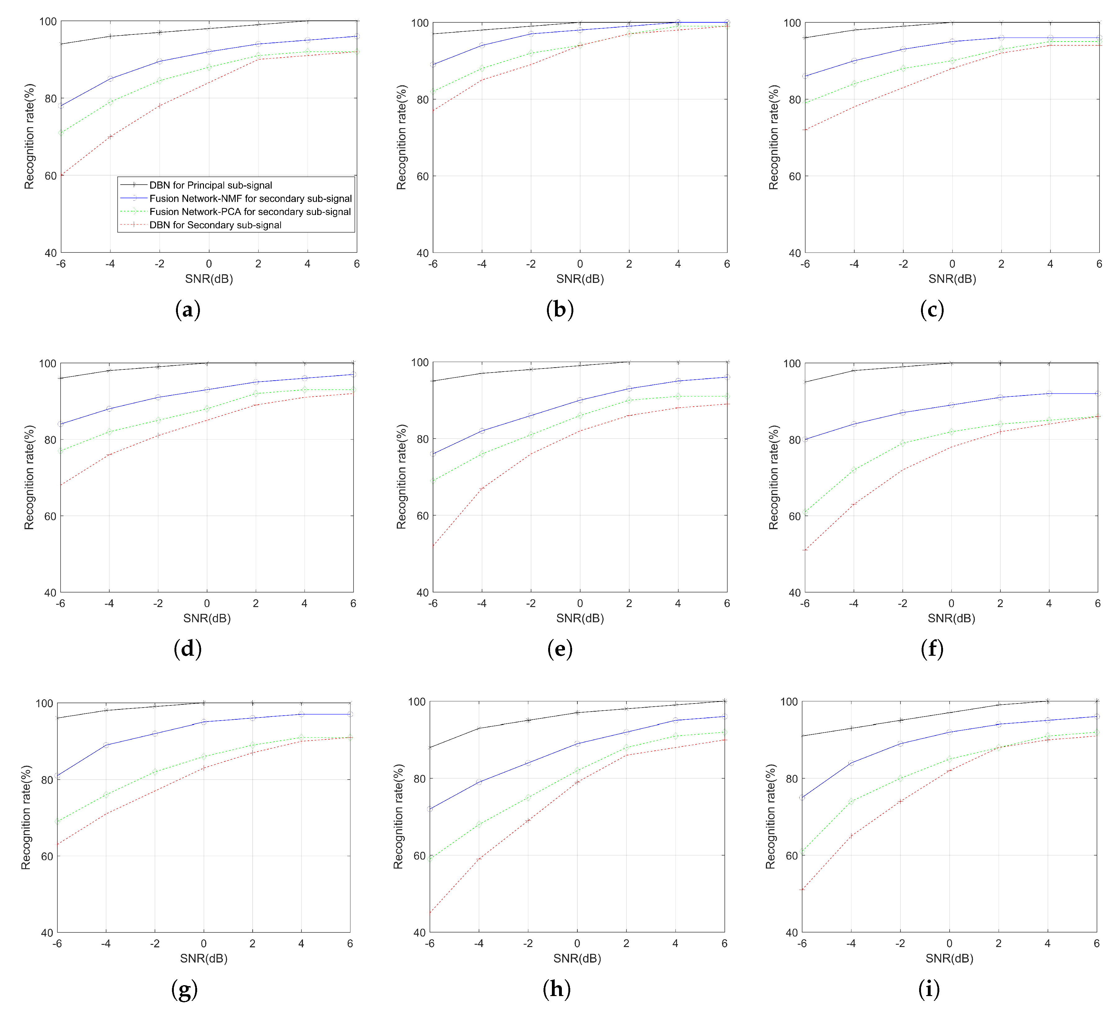
Figure 11 shows the performance of applying different networks to recognize each sub-signal. The black solid lines represent the recognition rate of the principal sub-signals by the proposed DBN technique. The blue solid lines represent the recognition rate of the secondary sub-signals by the proposed fusion network. The recognition rate of the fusion network combined with PCA and DBN for the secondary sub-signals are denoted by the green and red dotted lines, respectively.
With the improvement of SNR, the recognition rate of all methods gradually improved. Whether it is a low SNR or a high SNR, the proposed DBN technology achieves an ideal recognition rate in recognizing principal sub-signals. For secondary sub-signals, compared with the DBN and the fusion network combined with PCA, the proposed fusion network can achieve a better recognition rate at any SNR and a 94% overall recognition rate at an SNR of 0 dB. We also note that the gap between them decreases with the increase of SNR. In addition, the proposed fusion network is far superior to the above two technologies in recognizing polyphase codes, especially at a low SNR. In conclusion, these results show that the proposed fusion network has unique advantages in recognizing secondary sub-signals.
It is worth mentioning that the recognition rates of various signals as principal sub-signals are insensitive to noise. This phenomenon is due to the integrity of the principal sub-signals after RVMD. With the increase in SNR, the separation effect of each sub-signal is better; the energy loss of the secondary sub-signal is smaller. Therefore, the feature extraction advantage of the DBN is re-established. Multiphase codes have high similarity in shape and contour, which results in a low recognition rate of separated polyphase codes in the DBN. The advantage of the fusion network is that it combines the powerful image detail expression ability of Resnet50 with the premise that the DBN cannot obtain basic features of the signal. It is worth mentioning that, compared with the proposed fusion network using an NMF, the recognition rate of the fusion network combining PCA is worse, which is due to the strong characterization of image features by NMF.
4.4. Runtime Performance of the Proposed Method
As is known to all, besides the recognition rate, the key index of signal recognition technique is computational burden. Three groups are selected randomly. and 100 samples are selected for each group to test the running time of adaptive precise separation when the SNR is −4 dB, 0 dB, and 4 dB.
Table 3 shows the running environment.
Table 4 depicts the test results for recognizing per double signals with and without SVR.
Table 4 shows the time required to process the test signals. Note that there is a slight difference in the time required to recognize signals of different combinations, which is due to the difference in the parameter selection of the VMD, resulting in different separation time. The average running time for adaptive separation of multiple signals and accurate recognition of sub-signals is 2.23 s. In addition, we also test the technique without SVR under the same conditions, and the average running time is 37.17 s. Obviously, the fast regression ability of SVR has made a great contribution to shortening the time needed for recognition.
It is worth mentioning that there is currently no technology that can integrate signal separation and recognition. Therefore, the proposed technique really achieves rapid and accurate adaptive recognition of mixed signals. Moreover, the running time of the proposed method is not sensitive to the signal type and SNR, and the running time is relatively stable in general. The experimental results show that the proposed technique can find the optimal parameters of VMD in a short time, and the application of fusion network technique to recognize signals is faster than the current popular CNN.


