Abstract
To improve the positioning accuracy of an inertial/geomagnetic integrated navigation algorithm, a combined navigation method based on matching strategy and hierarchical filtering is proposed. First, the PDA-ICCP geomagnetic matching algorithm is improved. On basis of evaluating the distribution of magnetic measurements, a number of controllable magnetic values are regenerated to participate in the geomagnetic matching algorithm (GMA). As a result, accuracy of the matching algorithm is ensured and its efficiency is improved. Secondly, the integrated navigation filter is designed based on the hierarchical filtering strategy, in which the navigation information of the geomagnetic matching module and inertial navigation module are respectively filtered and fused in the main filter. In this way, the shortcoming that GMA is unable to provide continuous and real-time navigation information is overcome. Meanwhile, precision of the inertial/geomagnetic integrated navigation algorithm is improved. Finally, the feasibility and validity of the proposed algorithm are verified by simulation and physical experiments. Compared with the integrated filtering algorithm which directly uses the error equation of inertial navigation system (INS) as the state equation, the proposed hierarchical filtering algorithm can achieve higher positioning precision.
1. Introduction
An inertial navigation system (INS) can provide continuous and real-time navigation information for the carrier, and it is characterized by strong autonomy and good concealment. However, the navigation error of INS will accumulate over time, therefore it is hard to adapt to a long endurance mission. On the other hand, geomagnetic navigation is based on Earth’s geophysical field, which is passive, radiation-free and displays good stealth. Most importantly, the location error of geomagnetic navigation does not accumulate over time [1,2,3,4]. Therefore, constructing an inertial/ geomagnetic integrated navigation system can not only overcome the disadvantages of INS, such as accumulated navigation errors and poor long-term stability, but also can realize all-weather and all-region navigation.
According to their different combinations, inertial/geomagnetic integrated navigation algorithms can be divided into two categories, namely the loose and tight navigation algorithm. Generally speaking, the loose navigation algorithm mainly consists of the geomagnetic matching algorithm (GMA) and integrated navigation algorithm (INA), in which the locations evaluated by the GMA are used as observations of the integrated filter to estimate INS’s error [5]. The structure of loose navigation is beneficial for fault diagnosis, and is convenient for adding other navigation subsystems, but its filtering accuracy is largely affected by the location precision of GMA. As for the tight navigation algorithm, the measured magnetic values are directly used as observations of the integrated navigation filter [6]. As the measurement equation of tight navigation system is always nonlinear [7,8], the Extended Kalman Filter (EKF) [9], Unscented Kalman Filter (UKF) [10] and Particle Filter (PF) [11,12,13] are most commonly used. A linear approximation of the geomagnetic map is needed in EKF and UKF, but not for PF. Considering the non-linearity of the geomagnetic map, the EKF may easily diverge. Secondly, when other navigation subsystems are added, the loose INA is easier to implement.
It should be noted that the GMA is the core of loose INA, which estimates the carrier’s position by matching the geomagnetic characteristics measured in real time with the geomagnetic map previously stored in the navigation computer. Once the accuracy of the magnetic map is fixed, GMA is mainly affected by the magnetic measurements. Generally, the geomagnetic measurement error includes the instrument error, which is caused by the structure and materials of the magnetometer [14] and the interference field error, which is caused by the superposition of external interference field. Among them, the external interference field is mainly led by the hard and soft magnetic material of the carrier, and the random magnetic field which is difficult to describe using the magnetic model. In general, the non-random interference field in geomagnetic measurement can be processed by model compensation algorithms, but for the random interference field and other unknown interference factors that may appear in practice, the compensation result is always unsatisfactory. Currently, there are two ways to solve the problem: (1) In order to reduce the influence of interference field, process the magnetic measurements, such as Hilbert-Huang transform (HHT) [15], wavelet transform [16] and so on. (2) To study new GMA with good robustness.
The Iterated Closest Contour Point (ICCP) algorithm is a common method in geomagnetic matching, whose basic principle is shown in Figure 1. As is illustrated, suppose the matching length of ICCP algorithm is 5; C1 to C5 are five geomagnetic contour lines of a navigation area; M1 to M5 denote the real trajectory of the carrier; the carrier’s coordinates offered by the reference navigation system (usually the INS) at the sampling points are denoted by I1 to I5.
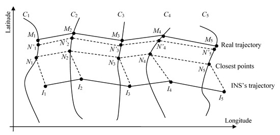
Figure 1.
Basic principle of ICCP algorithm.
If there is no magnetic interference, point Mn (n = 1, 2, …, 5) must be located on a geomagnetic contour line, but on which point of the contour is unknown. At the first step of geomagnetic ICCP algorithm, it finds the points closest to INS’s trajectory on the contour lines. The closest points are represented by N1 to N5 in Figure 1. Then ICCP algorithm will calculate the rigid transformation T (including rotation and transformation) between In and Nn (n = 1, 2, …, 5). Afterwards, the transformation T is applied to INS’s trajectory, and the new trajectory is denoted by N’1 to N’5. In next interaction, a new transformation will be used to minimize the distance between N’n (n = 1, 2, …, 5) and their closest points. The criterion to measure the distance between the points is in Formula (1). The above process will be iterated many times. Finally, In will continuously approximate the real trajectory of the carrier.
where d measures the distance of In and its corresponding contour line Cn.
The ICCP algorithm assumes that the magnetic sensor has no measurement error, and the real position of the carrier is located on or very close to the magnetic contour that corresponds to the magnetic measurement [17]. If the hypothesis is not satisfied, the accuracy of GMA would be hard to guarantee. Wu proposed a GMA based on the tree searching algorithm. It does not need to consider the distribution of measurement errors and has a certain anti-interference ability [18]. Xiao combined the probability data association (PDA) algorithm with the ICCP algorithm [19,20] and proposed a PDA-ICCP algorithm. It regarded all measurements of the magnetometer within a certain confidence range in interference environment as the effective measurements of a position, and finally evaluated the carrier’s location with the PDA fusion algorithm. The algorithm comprehensively considered the effects of measurement error and interference field and improved the GMA’s adaptability to a practical environment.
To guarantee the accuracy of the integrated inertial/geomagnetic navigation under interference environment, the PDA-ICCP algorithm is improved in our study and on basis of it, a new integrated navigation filter is designed. Finally, the feasibility and effectiveness of the proposed algorithm are verified through simulation physical and experiments.
2. Improvement of PDA-ICCP Algorithm
2.1. RM-PDA-ICCP Geomagnetic Matching Algorithm
In practice, due to the influences such as residuals of geomagnetic compensation, diurnal variation of magnetic field and measurement error of magnetometer, the magnetic measurement may not be equal to the corresponding value read from the geomagnetic map. If these magnetic measurements with noise are directly applied in GMA, the matching precision will be reduced. Even worse, it may lead to matching failure. To solve the problem, a PDA-ICCP algorithm is presented. Its basic idea is shown in Figure 2.
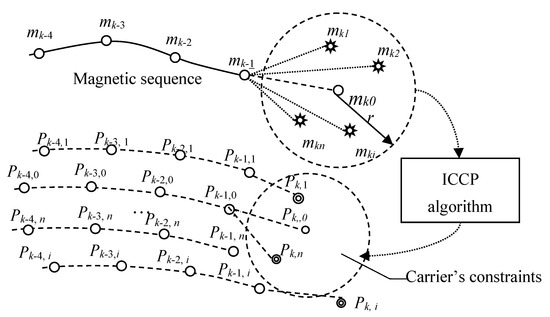
Figure 2.
Basic idea of PDA-ICCP algorithm.
As is illustrated in the figure, it is supposed that the matching length is 5. mk0, which is usually read directly from the magnetic map, is the ideal magnetic value at the kth matching point. mk1, mk2, …, mkn are the data measured n times at the kth point when interference field exists. mk-1, mk-2, …, mk-L+1 are the magnetic values of the other points of the geomagnetic matching sequence (GMS). Assuming the interference field follows the Gaussian distribution with mean 0, variance σ2, then according to the 3σ criteria, the magnetic measurements will fall within the circle of radius 3σ centered at mk0 with the probability of 99.74%. If the n measurements at the kth matching point are all within this circle (the upper circle in Figure 2), and each of them constitutes a GMS with mk-1, mk-2, …, mk-4, then there will be n matching results at kth point (denote as Pk, i, i = 1, 2, …, n) when the ICCP algorithm is executed. Considering the constraints of carrier’s kinematic performance, such as the heading and velocity constraints, its position should be within a reasonable scope. We denote the matching results in the scope as the valid estimations of the carrier’s location. Otherwise, the matching results are invalid. Finally, by fusing all valid estimations with PDA algorithm, the carrier’s final position can be estimated.
The essence of the method above is to select the positions where the carrier is most likely to appear and fuse them by PDA algorithm. In a statistical sense, if the magnetic field is measured enough times, there will always be a measurement close to the ideal magnetic value, thus the fusion effect of PDA algorithm is guaranteed. But, the more the ICCP algorithm is conducted, the worse the real-time performance it shows. In fact, if the magnetometer’s measurements are far away from the corresponding values read from the magnetic map, mismatches will appear in the GMA. These mismatched results are very likely to be eliminated due to the constraint of carrier’s motion in the fusion process of PDA. In other words, if number of the effective measurements is controllable and they are very close to the ideal geomagnetic value of the corresponding position, both the algorithm’s precision and real-time performance can be guaranteed. Based on this, an improved fusion algorithm based on regenerated measurements is put forward, which modified the first process of the PDA-ICCP algorithm to generate magnetic measurements. Its principle is shown in Figure 3:
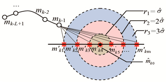
Figure 3.
Basic idea of RM-PDA-ICCP algorithm.
In Figure 3, the definition of mk-1, mk-2, …, mk-L+1 are the same with that in Figure 2, is the estimation of the ideal magnetic value at the kth matching point, is the estimated standard deviation of the magnetic measurements. Three circles, which are centered at with the radius of , 2 and 3, divide the confidence region of the magnetic measurements into three areas. RM-PDA-ICCP algorithm respectively regenerates several possible measurements in each area, which are denoted as m’k1, m’k2, …, m’km. They reconstitute the GMSs with the former L-1 matching points and participate the subsequent geomagnetic matching and fusion. To distinguish from the magnetic measurements in PDA-ICCP algorithm, these regenerated magnetic values are recorded as the regeneration measurements (RMs).
Rather than directly using the measured magnetic values for matching, the RM-PDA-ICCP algorithm regenerates a number of controllable RMs based on the statistical characteristics of the magnetometer’s measurements, which limits the number to execute the algorithm and enhances its real-time performance to a large extent. In addition, the RMs in r1, r2 and r3 can be adjusted to ensure the algorithm’s accuracy and the stability of the algorithm.
It can be concluded that the RM-PDA-ICCP algorithm contains the following steps:
- Firstly, estimate and , and regenerate the RMs.
- Secondly, conduct the ICCP algorithm with all the RMs.
- Thirdly, select effective matching results with the constraints of the kinematic performance of the carrier.
- Finally, calculate the associated probability and fuse all effective matching results.
Obviously, evaluating and , determining the constraints of carrier’s kinematic performance and calculating the associated probability of PDA algorithm are the key points in the RM-PDA-ICCP algorithm, which are explained respectively in the following parts.
2.2. Calculation of and
mk0 is the ideal magnetic value at a position in the PDA-ICCP algorithm, which is hard to achieve when the position error is very large. It is also challenging to measure the magnetic field of a position for many times while the carrier is moving. Nevertheless, measurement of the magnetometer is a random variable that follows a certain probability distribution. In addition, the carrier cannot move for a long distance within a short period, so the corresponding changes of the magnetic field are relatively small. In this sense, the magnetometer’s measurements within a short period can be considered as the random quantity of the measurements at a position, and the parameter estimation method can be used to evaluate the statistical characteristics of the magnetic measurements.
Suppose mk1, mk2, …, mkn are the values measured n times at the kth matching point, and they follow the Gaussian distribution, then according to the moment estimation method, the estimated value of mk0 and σ2 can be expressed as:
2.3. Constraints of Carrier’s Kinematic Performance
The position of the carrier at the kth matching point can be estimated by its kinematic performance at the (k-1)th matching point. As is shown in Figure 4, (xk-1, yk-1) and (xk, yk) respectively denote the carrier’s position at the (k-1)th and kth matching point. Considering the influence of velocity error and course error, and supposing the carrier’s velocity and course interval at (k-1)th point is [,] and [,], then at the kth point the carrier is restricted within the concentric circles with the radius of and by the velocity error, and in a fan-shaped area by the course error. Here, variable T measures the time between (k-1)th and kth point. Finally, the shadow part in Figure 4 shows the possible position of the carrier, which can be described by Formula (3).
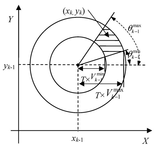
Figure 4.
Constrains of carrier’s movement on the matching results.
2.4. Calculation of the Associated Probability
Associated probability determines the fusion coefficient of every effective position restricted by Formula (3). Suppose the n measurements (mk1, mk2, …, mkn) at the kth matching point follow the normal distribution with the mean of mk0 and variance of σ02, then the probability Prki that the ith measurement derives from its ideal magnetic value can be expressed as:
where erf(x) is the error function and is defined as:
Define a matrix (A)1×n, where n is the measurement number at the kth matching point. Once the matching result of the ith measurement satisfies Formula (3), the ith element in A is set to 1. Otherwise, the corresponding element is 0. As a result, the associated probability of each effective matching result, denoted by (i = 1, 2, …, n) can be represented as:
Normalize , then the associated probabilities are:
Finally, the position of the carrier is estimated as:
where is the final position estimated by the RM-PDA-ICCP algorithm, Pk,i is the matching result of ICCP algorithm corresponding to the ith magnetic measurement mki.
3. Design of the Integrated Navigation System
According to different state variables, the loose integrated navigation algorithm can be divided into two types: the one based on position error [2] and the one based on location (and speed) [5]. The former usually takes the error equation of INS as the state equation of the integrated navigation filter, and the position error of GMA as the observations to estimate the attitude error, velocity error and position error of the carrier. While the latter directly takes the motion equation of the carrier as state equation, and updates the position and speed immediately. The above two integrated algorithms have been applied in integrated navigation system that based on geophysical fields such as geomagnetism, gravity and terrain. In our study, a hierarchical filter is put forward. The inertial/geomagnetic integrated navigation system is designed in Figure 5, which adopts the carrier’s location as the state variable. As is shown, the hierarchical filter is divided into two layers, the first layer consists of two subfilters, and the second one includes a main filter.
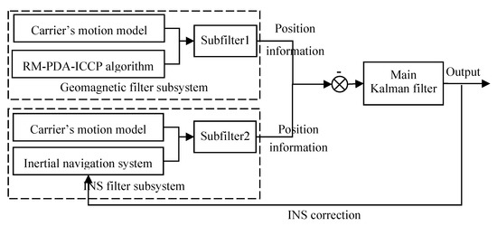
Figure 5.
Inertial/geomagnetic integrated navigation system.
The above system consists of two sub-filters and one main filter. First, the geomagnetic and inertial navigation subsystems independently execute the Kalman filtering algorithm and give an estimate of the carrier’s position. Then the main filter integrates the position information of two subsystems to evaluate the position error and velocity error of the carrier. Ultimately, the INS can be corrected. In the following, the state equation, measurement equation and filtering algorithm of the integrated navigation system are described in detail.
3.1. State Equation and Observation Equation of the Subsystem
Assume the carrier is in the uniform rectilinear motion, the matching results of GMA are taken as observations of the filter, and the position and velocity in longitude and latitude are taken as the state, namely , then the state equation and observation equation of the geomagnetic filter subsystem can be expressed as:
where , , , T is the time between two sampling points, Uk is the random disturbance during the movement of the carrier, Vk is the location estimation noise of GMA.
The RM-PDA-ICCP algorithm executes once a magnetic measurement is obtained. In the regions where the geomagnetic fluctuation is not very obvious, the RM-PDA-ICCP algorithm is prone to mismatching. If the mismatched results are sent to the main filter, the precision of integrated navigation system will greatly reduced. In this sense, the geomagnetic filter subsystem will evaluate a proper result for the main filter. Finally, the accuracy and real-time performance of the integrated navigation algorithm are ensured.
The state and observation equation of the inertial subsystem are the same as the geomagnetic filter subsystem, which are not discussed to keep our study concise.
3.2. State Equation and Observation Equation of the Main Filter
In the main filter, the position difference between two subsystems is taken as the observation. Its state equation and observation equation are:
where , wk is the system noise; λGMNS and λINS are the matching position of the geomagnetic filter subsystem and inertial subsystem in longitude respectively, LGMNS and LINS are the positions in latitude. nk is the location estimation noise, , .
3.3. Integrated Filtering Algorithm
As the state and observation equations of the integrated navigation system are all linear, a standard KF algorithm can be adopted. The difference between the subfilters and main filter is that a threshold is set in the geomagnetic filter subsystem to restrict the matching results whose error is very large. The filtering and updating process of the geomagnetic filter subsystem is shown in Figure 6, in which Q and R stand for the variance of the process noise Uk and measurement noise Vk; Zk is the observation, which is corresponding to the matching results of RM-PDA-ICCP algorithm. P0 and are the initial states of filtering; P is the covariance matrix, K is the filtering gain matrix, and is the state estimation of the subsystem. Other variables are the same with that in Formula (9)–(12).
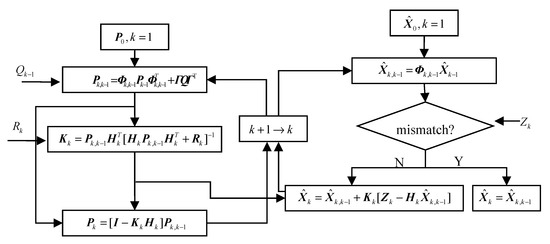
Figure 6.
Filtering process of the geomagnetic filter subsystem.
In Figure 6, the covariance matrix, gain matrix and filtering state are updated during the filtering process. If the observation Zk exceeds the presupposed threshold, the estimated state should be taken as current state , otherwise should be updated with the KF algorithm. The filtering process of the main filter is a standard KF.
In essence, the algorithm above belongs to the loose integrated navigation algorithm. Furthermore, only minor changes are needed when other auxiliary navigation methods are added to the integrated navigation system. In addition, introducing filtering algorithm to the geomagnetic matching module is beneficial to improve the adaptability to the geomagnetic environment.
In a word, the proposed algorithm can be summarized as follows:
- Step 1: To execute the RM-PDA-ICCP algorithm and obtain the estimated position of the carrier;
- Step 2: The result in Step 1 is taken as the observation of the geomagnetic filter subsystem;
- Step 3: The information offered by the inertial system is used in the INS filter subsystem;
- Step 4: The results of Step 2 and Step 3 are fused by the main filter. Finally, the positions of the carrier are continuously calculated.
4. Simulation Experiments
A local area of the magnetic anomaly field is randomly selected from the Y component of the NGDC-720 model to verify the proposed algorithm, its latitude and longitude respectively ranging from [49.8°, 50.8°] N and [36.5°, 37.5°] E. Then the Kriging interpolation method is used to establish the detailed magnetic map, as is shown in Figure 7. After interpolation, the resolution of the geomagnetic map is about 100 m.
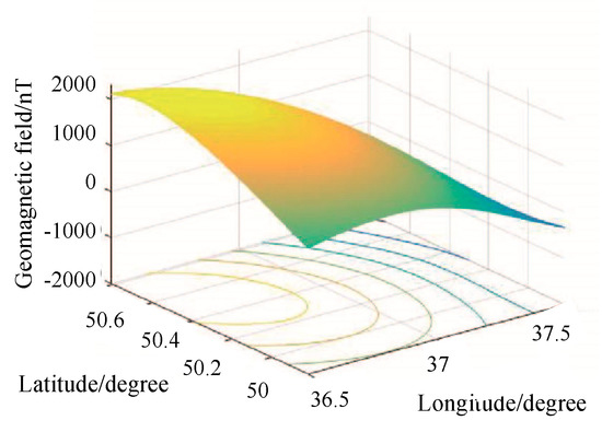
Figure 7.
The geomagnetic field of a mission area.
4.1. Effectiveness of the Proposed Algorithm
It is assumed the carrier is in uniform rectilinear motion, and the angle between its movement direction and X-axis is 135°. It’s velocity along the East and north are both 15 m/s. Suppose the proposed integrated navigation algorithm is conducted from the point [37.4° E, 49.86° N]. INS’s accumulated error is simulated by adding different rigid transformations to the real trajectory [21]. The measurement error is Gaussian white noise. Its original position errors in longitude and latitude are both 300 m, and the bias of gyroscope is 1 °/h. Suppose the magnetic interference follows the normal distribution, whose average is 0 nT and variance is 1 nT2.
Evaluate mk0 and σ2 by the method in Section 2.2, and then ten RMs at ± 1/4, ± 1/2, ± , ± 2 and ± 3 could be generated respectively. Assume the matching length of GMS is 5, and the allowable velocity error and course error of the carrier are respectively ±5 m/s and ±20°, then the RM-PDA-ICCP algorithm is conducted. If all matching results corresponding to the RMs do not meet the constraint of carrier’s kinematic performance, the algorithm does not output.
Afterwards, Formula (9) and (10) are used in the geomagnetic filter subsystem, where the matching results of RM-PDA-ICCP algorithm are taken as the observations, and the position and velocity are the filter’s state. The sampling interval is T = 2 s, and the location estimation noise covariance R and process noise covariance Q are set as follows:
where the unit of R is (m)2. In matrix Q, units of the elements representing the position are (m)2, units of the elements representing velocity is (m/s)2.
Since the matching length is 5, namely the matching result of RM-PDA-ICCP algorithm is output from the 5th sampling point, therefore the filtering initial value of the geomagnetic subsystem is set to X(4), and the initial covariance is:
where the unit of P0 is defined the same as that in matrix Q.
In order to quantitatively describe the effect of GAM and filtering algorithm, the total position error is defined as:
where (, ) is the estimated location at sampling point k, and (λk, Lk) is the real position of the carrier.
Figure 8. shows the filtering results of the geomagnetic navigation subsystem. It can be seen that although the matching results of RM-PDA-ICCP algorithm are effective at most sampling points, the matching errors are relatively large. When the filtering algorithm is conducted, the positioning accuracy of the geomagnetic filter subsystem is significantly improved. As is shown in Figure 8c, all positioning error is within 250 m, whereas the accuracy still needs to be improved.
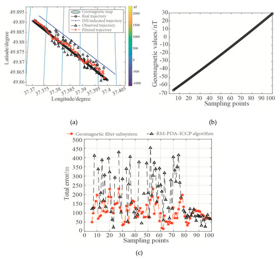
Figure 8.
Filtering results of the geomagnetic filter subsystem: (a) Filtering trajectory of geomagnetic filter subsystem; (b) The magnetic values along the trajectory; (c) Total filtering error of geomagnetic filter subsystem.
In addition, it is obvious that the outputs of RM-PDA-ICCP algorithm in Figure 8a are not continuous, and the position errors at some sampling points in Figure 8c are not displayed (such as the 45th sampling point). This is because the matching results corresponding to all RMs are too large to meet the constraint of carrier’s kinematic performance.
For the inertial subsystem, m. Other simulation parameters are the same as the geomagnetic filter subsystem. Figure 9 shows its filtering results.
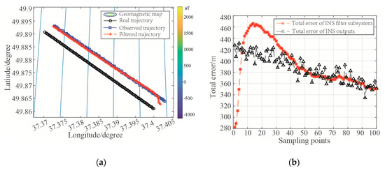
Figure 9.
Filtering results of the INS filter subsystem: (a) Filtering trajectory of the INS filter subsystem; (b) Total location error of the INS filter subsystem.
As is shown in the illustration, filtering results of the inertial subsystem change with the outputs of INS. However, considering the influence of INS’s accumulated error, the filtering result will diverge over time. Therefore, even if the filtering algorithm is applied, the geomagnetic filter subsystem still calls for correction.
Based on the filtering results of the geomagnetic and inertial subsystem, the main filter is established according to Formula (11) and (12). Other simulation parameters are the same as the geomagnetic filter subsystem. Figure 10 gives the filtering results of the integrated navigation system:
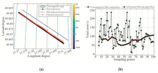
Figure 10.
Filtering results of the integrated navigation system: (a) Filtering trajectory of the integrated system; (b) Total error of the integrated system.
In Figure 10a, the filtering results of two subsystems are further integrated in the main filter. Obviously, the position accuracy is greatly improved. In Figure 10b, it shows the total error at each sampling point is less than 120 m, which is much better than the subsystem.
Table 1 lists some statistical characteristics of the location error of each system. The results are consistent with the above analysis.

Table 1.
Results of simulation experiment (Unit: m).
4.2. Algorithm Comparison
To further validate the proposed integrated navigation algorithm, comparison experiments are conducted in this section. First, set the original error of INS in latitude and longitude to 200 m, its total error is 282.8 m (about 2.82 magnetic grids). R and Q are set according to the actual equipment: the magnetic measurement error is based on the performance of the magnetometer; the error of INS is referenced to the parameters of a certain type of unmanned aerial vehicle (UAV). For the sake of privacy, the values are not exactly the same with actual equipment, but by experiment comparison, the conclusion still holds. Other simulation parameters are the same as that in Section 4.1. Then, the proposed algorithm is compared with the other loose integrated navigation algorithm, which takes the error equation of INS as state equation and the matching error as observation [2]. Its state and observation equation are shown below:
where , , and stand for the attitude angle error in north, up and east, corresponds to the velocity error in north and east, and are the position error in longitude and latitude; F is the state transfer matrix of INS’s error equation; mk is the system noise. F is the state transition matrix when the error is taken as the state variable, and a traditional Kalman filtering method is adopted. The detailed principle can refer to reference [22]; δrk represents for the location error of RM-PDA-ICCP algorithm, .
Figure 11 shows the comparative results:
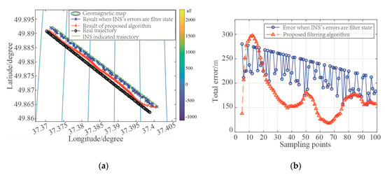
Figure 11.
Filtering results of integrated navigation system: (a) Filtering trajectories of different algorithms; (b) Total location error of different algorithms.
As is illustrated in the figure, the filtering results of different algorithms are located near the real position of the carrier, indicating that both algorithms are effective. But comparatively speaking, the total error of the proposed integrated navigation algorithm is less than 200 m (2 magnetic grids) when the filter is stable, and its positioning result is much closer to the real position of the carrier.
5. Flight Experiment
Considering the magnetic field in the air is relatively pure, a quadrotor is used in our study to test the proposed integrated navigation algorithm. The experiment system is shown in Figure 12.
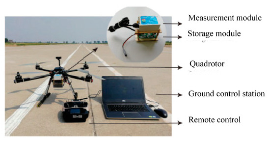
Figure 12.
Experiment system of INS/integrated navigation system.
As is shown, the inertial/geomagnetic integrated navigation system mainly includes the following parts: the measurement and storage module, the quadrotor and the ground control station. Among them, the measurement module is a 10-axis high precision attitude-angle sensor made by Wit Smart Company, which contains the RM3100 geomagnetic sensor, inertial element and GPS module. Its main parameters are listed in Table 2. The storage module uses a serial port to SD card to storage data. To avoid the influence of carrier’s material on the magnetic measurement, the frame of the quadrotor is made of carbon.
Table 2.
Main parameters of the sensor module.
In the system, the real position of the carrier is given by GPS; the ground control station is used to communicate with the quadrotor, to load the planed trajectory and to conduct the integrated navigation algorithm.
The total magnetic values of the sensor are applied in navigation. Finally, a measured geomagnetic field with the size of 1400 m × 600 m is taken as the background, whose grid resolution is 25 m. The quadrotor is in the uniform rectilinear motion at the speed of 5 m/s with the starting point being (199.3 m, 201.5 m) and altitude 40 m. Suppose the baud rate of sensor module is 9600, its output frequency is 10 Hz. Limited by the endurance time of the quadrotor, the INS element has worked for a while before the flight experiment, so its accumulated error is obtained. Assume the original position errors of INS in longitude and latitude are both 40 m, namely the total error of INS is 56.57 m (about 2.26 magnetic grids), bias of the gyro is 1 °/h.
Then the proposed integrated navigation algorithm is executed. In the geomagnetic filter subsystem, the state and observation equation follow Formula (9) and (10), where T = 5 s. The variance matrix of the observation noise , and the process noise .
In the main filter, the process noise . Other parameters are unchanged. Figure 13, Figure 14, Figure 15 and Figure 16 respectively show the filtering results of the geomagnetic filter subsystem and the integrated navigation system, and Table 3 lists some statistical characteristics of the location error of each system.
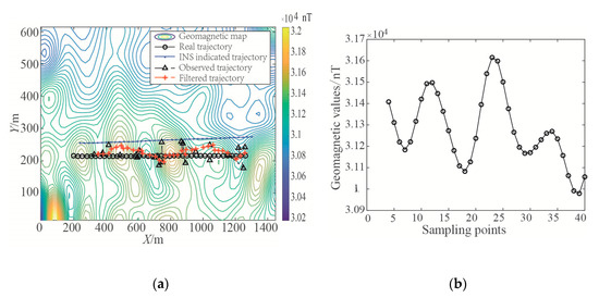
Figure 13.
Geomagnetic filtering result. (a) Filtering results of the geomagnetic filter subsystem; (b) The magnetic values along the trajectory.
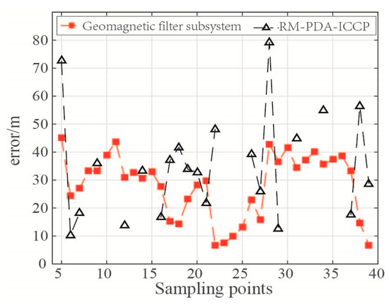
Figure 14.
Total error after geomagnetic filtering.
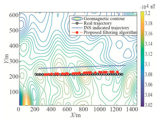
Figure 15.
Filtering result in flight experiment.
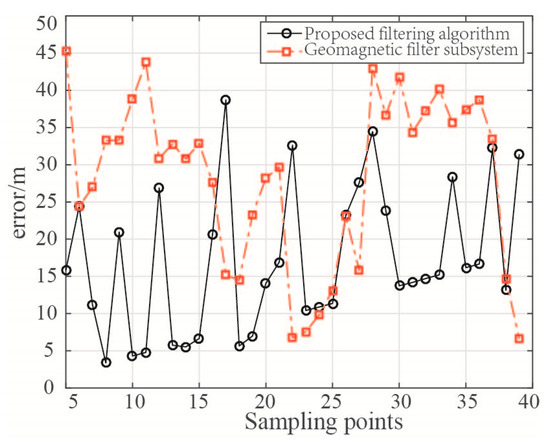
Figure 16.
Total error of integrated system.
Table 3.
Results of flight experiment (Unit: m).
In Figure 14, as all matching results corresponding to the RMs are beyond the threshold of effective matching, the RM-PDA-ICCP algorithm has no output at some sampling points. Besides, the matching errors at some points are too large, for example the 5th and the 28th sampling points. However, the total location error of the subsystem after filtering is within 50 m (about 2 magnetic grids). As a result, the locations of the carrier could be output continuously by the geomagnetic filter subsystem. Comparing the final filtered trajectory with the carrier’s real trajectory in Figure 13a, it is shown that the observations have a great influence on the filtering algorithm.
In Figure 15 and Figure 16, the filtering trajectory of integrated navigation system is very close to carrier’s real trajectory, and all the total filtering errors are less than 40 m (about 1.6 magnetic grids). Compared with the geomagnetic filter subsystem, the filtering results are obviously improved. This result proves the effectiveness of proposed combined navigation algorithm.
6. Conclusions
Filtering accuracy of the integrated navigation system is greatly impacted by the results of GMA. Due to the precision limitation of geomagnetic measurements and mapping, and the magnetic information in some areas being insufficient, the GMA is easy to mismatch. The RM-PDA-ICCP algorithm fuses each possible matching within a certain confidence region and improves the reliability of the location result. In addition, the hierarchical filtering and refusion strategy is able to fuse the results of each navigation subsystem, which guarantees the advantages of loose integrated navigation system and improve its accuracy at the same time.
In order to reduce the influence of the magnetic field of the carrier on magnetic measurements, the frame of the quadrotor is carbon. However, there are a lot of ferromagnetic materials and electromagnetic equipment in the actual system and as a result, the proposed integrated navigation algorithm will be further verified based on magnetic measurement compensation.
Author Contributions
X.D., J.X., and X.Q. conceived and designed the experiments; J.X. and Y.L. performed the experiments; X.D. and J.X. analyzed the data and wrote the paper.
Acknowledgments
Thanks for the financial support of Hebei Key Laboratory of UAV Detection Technology and Application, which is affiliated with Zhongke Hengyun Co., Ltd.
Conflicts of Interest
The authors declare no conflict of interest.
References
- Xiao, J.; Duan, X.; Qi, X.; Wang, J. Direction navigability analysis of geomagnetic field based on Gabor filter. J. Syst. Eng. Electron. 2018, 29, 378–385. [Google Scholar] [CrossRef]
- Goldenberg, F. Geomagnetic navigation beyond the magnetic compass. In Proceedings of the 2006 IEEE/ION Position, Location, and Navigation Symposium, Coronado, CA, USA, 25–27 April 2006; pp. 684–694. [Google Scholar]
- Shockley, J.A.; Raquet, J.F. Navigation of Ground Vehicles Using Magnetic Field Variations. J. Inst. Navig. 2014, 61, 237–252. [Google Scholar] [CrossRef]
- Canciani, A.J.; Raquet, F. Absolute positioning using the Earth’s magnetic anomaly field. In Proceedings of the 2015 International Technical Meeting of the Institute of Navigation, Tampa, FL, USA, 14–18 September 2015; pp. 265–278. [Google Scholar]
- Han, Y.; Wang, B.; Deng, Z.; Fu, M. An Improved TERCOM Based Algorithm for Gravity Aided Navigation. IEEE Sens. J. 2016, 16, 1. [Google Scholar] [CrossRef]
- Zhang, K.; Li, Y.; Zhao, J.; Rizos, C. A Study of Underwater Terrain Navigation based on the Robust Matching Method. J. Navig. 2014, 67, 569–578. [Google Scholar] [CrossRef]
- Stepanov, O.A.; Toropov, A.B. Nonlinear filtering for map-aided navigation. Part 1. An overview of algorithms. Gyroscopy Navig. 2015, 23, 102–125. [Google Scholar]
- Stepanov, O.A.; Toropov, A.B. Nonlinear filtering for map-aided navigation Part 2. Trends in the algorithm development. Gyroscopy Navig. 2016, 7, 82–89. [Google Scholar] [CrossRef]
- Wang, Z.; Bian, S. A local geopotential model for implementation of underwater passive navigation. Prog. Sci. Mater. Int. 2008, 18, 1139–1145. [Google Scholar] [CrossRef]
- Ning, X.; Huang, P.; Fang, J.; Liu, G.; Ge, S.S. An adaptive filter method for spacecraft using gravity assist. Acta Astronaut. 2015, 109, 103–111. [Google Scholar] [CrossRef]
- Teixeira, F.C.; Quintas, J.; Pascoal, A. AUV Terrain-Aided Navigation using a Doppler Velocity Logger. IFAC-PapersOnLine 2015, 48, 137–142. [Google Scholar] [CrossRef]
- Gustafsson, F.; Gunnarsson, F.; Bergman, N.; Forssell, U.; Jansson, J.; Karlsson, R.; Nordlund, P.-J. Particle filters for positioning, navigation, and tracking. IEEE Trans. Signal Process. 2002, 50, 425–437. [Google Scholar] [CrossRef]
- Gustafsson, F. Particle filter theory and practice with positioning applications. IEEE Aerosp. Electron. Syst. Mag. 2010, 25, 53–82. [Google Scholar] [CrossRef]
- Heller, W.G.; Jordan, S.K. Error analysis of two new gradiometer-aided inertial navigation systems. J. Spacecr. Rockets 2015, 13, 340. [Google Scholar] [CrossRef]
- Liu, M.; Wang, H.; Gao, B. A submarine geomagnetic matchiing algorithm based on HHT noise reduction. Eng. Surv. Map. 2014, 23, 29–31. (In Chinese) [Google Scholar]
- Qiao, Y.; Zhang, J.; Sun, Y.; Wang, S. A method for geomagnetic matching navigation based on forced de-noising and multi-scale fusion. J. Astronaut. 2011, 32, 53–59. (In Chinese) [Google Scholar]
- Xie, W.; Li, Q.; Xi, B.; Huang, L.; Wang, C. Geomagnetic contour matching algorithm based on interative method. J. Chin. Inert. Technol. 2015, 23, 631–635. (In Chinese) [Google Scholar]
- Wu, Z.; Hu, X.; Wu, M.; Mu, H.; Cao, J.; Zhang, K.; Tuo, Z. An experimental evaluation of autonomous underwater vehicle localization on geomagnetic map. Appl. Phys. Lett. 2013, 103, 104102. [Google Scholar] [CrossRef]
- Xiao, J.; Duan, X.; Qi, X. An ICCP geomagnetic matching algorithm based on probability data association. J. Chin. Inert. Technol. 2018, 26, 202–208. (In Chinese) [Google Scholar]
- Xiao, J.; Duan, X.; Qi, X. An Adaptive △M-ICCP Geomagnetic Matching Algorithm. J. Navig. 2017, 71, 649–663. [Google Scholar] [CrossRef]
- Gulati, D.; Zhang, F.; Malovetz, D.; Knoll, A.; Clarke, D. Robust cooperative localization in a dynamic environment using factor graphs and probability data association filter. In Proceedings of the 2017 20th International Conference on Information Fusion (Fusion), Xi’an, China, 10–13 July 2017; pp. 1–6. [Google Scholar]
- Mackison, D.L. Review of Strapdown Inertial Navigation Technology. J. Guid. Control Dyn. 2015, 21, 1018. [Google Scholar] [CrossRef]
© 2019 by the authors. Licensee MDPI, Basel, Switzerland. This article is an open access article distributed under the terms and conditions of the Creative Commons Attribution (CC BY) license (http://creativecommons.org/licenses/by/4.0/).