Article

A Simplified Optimal-Switching-Sequence MPC with Finite-Control-Set Moving Horizon Optimization for Grid-Connected Inverter

1
New Energy Research Center, School of Electric Power, South China University of Technology, Guangzhou 510640, China
2
Dongguan DRN New Energy CO, LTD., Dongguan 523000, China
3
Guangdong Key Laboratory of Clean Energy Technology, School of Electric Power, South China University of Technology, Guangzhou 510640, China
*
Author to whom correspondence should be addressed.
Electronics 2019, 8(4), 457; https://doi.org/10.3390/electronics8040457
Submission received: 15 March 2019 / Revised: 13 April 2019 / Accepted: 22 April 2019 / Published: 25 April 2019
(This article belongs to the Section Power Electronics)

Abstract

:
Optimal-switching-sequence model-predictive-control (OSS-MPC) strategy, a popular kind of continuous-control-set MPC (CCS-MPC), has been used to address the variable frequency of finite-control-set MPC (FCS-MPC). Since the digital signal processor (DSP) does not have a dedicated divider, it requires a large amount of computation for the division operations in OSS searching. Here, a simplified OSS-MPC absorbing the merits of FCS-MPC is proposed to reduce the computational burden of conventional OSS-MPC. The proposed method uses a novel cost function whose candidates are the finite center vectors instead of switching sequences, which can avoid duty cycle computation and convert the moving horizon optimization of CCS-MPC into that of FCS-MPC. Besides, the derivatives of the active and reactive powers are divided into the constant terms and variable terms. The constant terms are extracted from the cost function. Experimental and simulation results show that the computational amount of the proposed algorithm is only 36.34% of that of the conventional OSS-MPC. Meanwhile, the simplified OSS-MPC still maintains the excellent dynamic and steady state performance of conventional OSS-MPC.

1. Introduction

Grid-connected inverter plays a key role in renewable energy systems, distributed generation systems, power quality improvement units, and so on [1,2]. Since the performance of the inverter depends largely on the control strategy, much effort has been done on the control strategy of the grid-connected inverter.
Classical control strategies of the grid-connected inverter can be mainly divided into two categories [2]. One is voltage oriented control (VOC) [3], which is broadly used for grid-connected inverters due to its good steady-state performance. Nevertheless, the inner current control loop and the proportional integral (PI) controllers may lower the dynamic performance of the system. The other is direct power control (DPC), which is based on the direct torque control (DTC) of AC machines [4,5], has been proposed to get better dynamic performance. However, it has variable switching frequency and large power ripples due to the predefined switching table.
Recently, a novel and computationally complex control strategy, model predictive control (MPC), has been proposed. The MPC shows a lot of advantages such as ease of implementation, flexibility in the definition of control objectives, and fast dynamic response [6,7,8].
Depending on the nature of the input constraints, model-predictive-control (MPC) can be divided into continuous control set (CCS) MPC and finite control set (FCS) MPC [9]. In FCS-MPC schemes, the inverter switching states are handled directly without using a modulator, and the input will belong to an FCS. Once a modulator is used, the input will be constrained to belong to a bounded CCS, which contains more than one switching state in a sampling period. Therefore, FCS-MPC only selects one switching state in a sampling period, which causes high power ripple and variable switching frequency [10,11]. Considering that CCS-MPC can acquire constant switching frequency by using the modulator [12]. The best-known algorithm in CCS-MPC is the predictive direct power control (P-DPC) based on the space vector modulation (SVM) whose vector sequence that contains two nonzero vectors and one zero vector is employed during every control period. Although conventional P-DPC can realize fixed switching frequency, its performance is deteriorated by incorrect vector sequence selection [13,14]. This is because the two nonzero vectors in vector sequence are selected according to the angular position of the grid voltage vector instead of the ideal output voltage vector. And the incorrect vector sequence might lead to the calculation of negative duration time, which would be clamped to zero in the practical system. To select the correct vector sequence, an improved vector sequence table has been proposed for P-DPC in reference [14], which can modify the optimal switching sequence when the duration time becomes negative. However, the control action of all these algorithms still require the grid voltage angle and an extra SVM.
To solve this issue, the CCS-MPC with optimal switching sequence (OSS-MPC) has been presented in references [15,16,17], substituting the vector sequences that contain more than one voltage vector into the cost function. Compared with P-DPC, the advantage of OSS-MPC is that it does not need grid voltage angle and can select the OSS even when the control action is saturated [15]. Since the OSS-MPC in a way resembles a modulator in the optimization problem, the duration time of the switching states are needed. However, the division of the duration time of the switching states will increase the computational burden of the microprocessor. Considering other functions in renewable energy sources that should be implemented in the sampling period, such as islanding detection protection or maximum power point tracking algorithm [18], the computational burden of the conventional OSS-MPC should be reduced.
Different from the classical OSS-MPC with two nonzero vectors and one zero vector in one sampling period, there is also OSS-MPC with two voltage vectors in one sampling period, which is called dual vector based MPC (D-MPC) [19,20,21]. These methods can mitigate the computational burden due to the less voltage vectors in one sampling period, and have a faster speed of moving horizon optimization. However, since D-MPC only contains two voltage vectors in the OSS, there is only one degree of freedom for the duration time control and the active and reactive power errors cannot be removed at the same time. In references [18,22], a constructed reference voltage vector in two-level and three-level converter has been applied in the cost function optimization for OSS-MPC. The reference voltage vector can select the OSS directly, thus reducing the cyclic number from 6 to 1. However, it needs a grid voltage angle to construct a reference voltage vector when it is connected to the grid, which partly deviates from the advantages of conventional OSS-MPC. There are many other algorithms that can alleviate the computational burden of other kinds of CCS-MPC [23,24] and FCS-MPC [25,26,27] but few about OSS-MPC. However, they are not suitable for our target (OSS-MPC for two-level grid-connected inverter) because of the difference between moving horizon optimization [23,24], or may sacrifice some advantages of OSS-MPC if they are introduced into OSS-MPC [25,26,27]. The lack of work concerning the computational efficiency of classical OSS-MPC is partly because it often damages the merit of OSS-MPC while reducing the computational burden. The related literature that can maintain the merit of OSS-MPC is reduced OSS-DPC (ROSS-DPC) [15], which reduces the computational cost by calculating the derivative of active and reactive power of the switching states before moving horizon optimization. In this way, the calculating times of the derivative of the active and reactive power can be reduced. However, this method has limited effect since the duration times of each vector need to be calculated, which still occupies a lot of computational cost during the minimization of the cost function.
This paper aims to propose a simplified OSS-MPC strategy, which can reduce the computational burden while maintaining all advantages of OSS-MPC. We introduce the core idea of FCS-MPC into OSS-MPC by constructing a new cost function with center vectors. The new cost function uses the center vectors to search the OSS and avoid the division operation in duration time calculation. And the duration time of OSS will be calculated after moving the horizon optimization. At the same time, the active and reactive power predictive model are divided into various parts and a constant part. Then the constant part is extracted from the moving horizon optimization thus as to decrease the computational amount further. In this way, the proposed algorithm can alleviate the computational burden of conventional OSS-MPC without sacrificing the excellent performance of it.
The main advantages of the proposed method are summarized as follows: (i) Compared with the D-MPC [19,20,21], the proposed strategy maintains three voltage vectors in one sampling period, and thus has a better steady state performance. (ii) Compared with the strategy introduced in reference [18], the proposed strategy does not require the grid voltage sector information. The OSS can be selected even when the control action is saturated [15]. (iii)Compared with ROSS-DPC [15], the proposed strategy can reduce the computational burden further.
The hypotheses of the study are given as follow. We assume that (i) the insulated gate bipolar transistors (IGBTs) are ideal switches; (ii) the resistance of the wires and the inductors (AC filter) can be ignored; (iii) the inverter is connected to a balanced and ideal grid.
The rest of this paper is organized as follows. Conventional OSS-MPC for grid-connected inverter is introduced in Section 2. In Section 3, the proposed algorithm is analyzed and its superiorities are summarized. In Section 4, the experimental platform is established to verify the effectiveness and advantages of the proposed algorithm. Finally, the conclusion is given in Section 5.

2. Conventional OSS-MPC

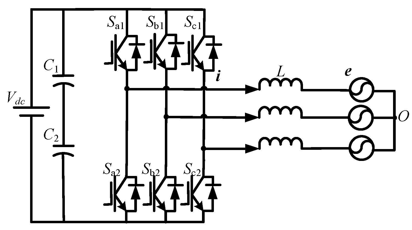
2.1. Model of Two-Level Grid-Connected Inverter
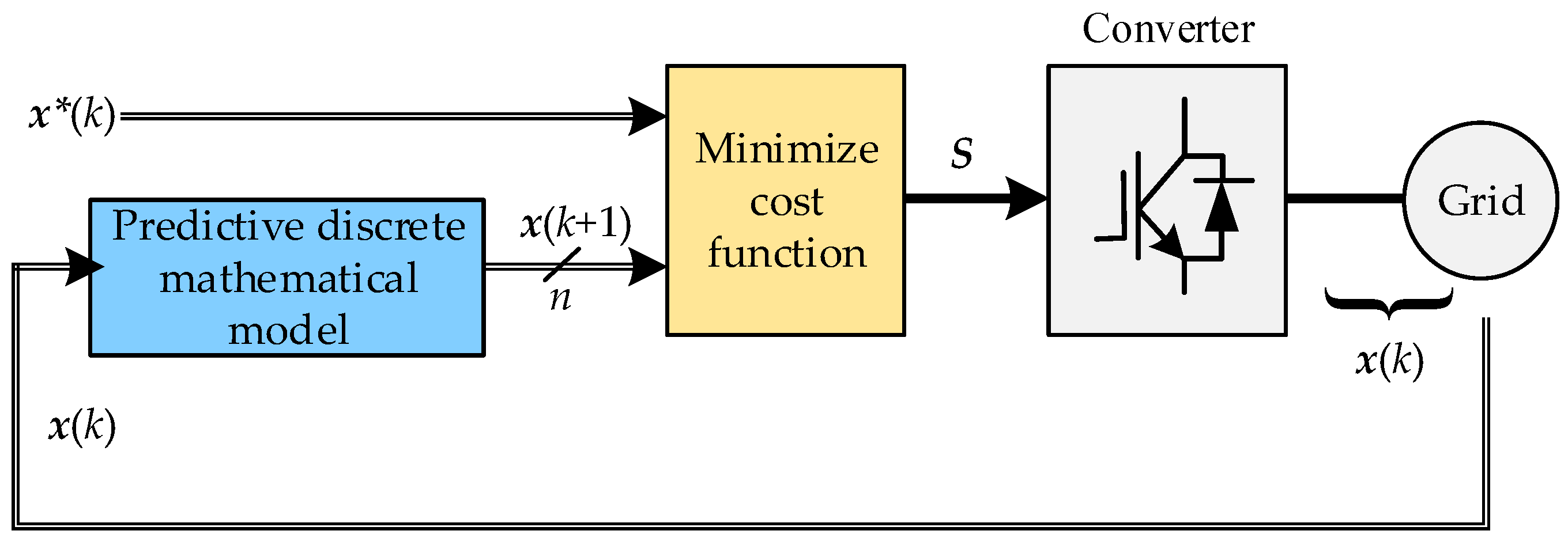
Figure 1 shows an exemplary two-level grid-tied inverter, which contains six insulated gate bipolar transistors (IGBTs) with antiparallel diodes. Vdc is the direct current (dc) power supply, e is the grid voltage, C1 and C2 are the dc-link capacitors. Additionally, L is the inductance of the AC filter.
As shown in Figure 1, SX1 and SX2 represent the upper and lower switching states of each phase, with x = a, b, c. Different switching states of each phase in inverter can produce different output voltages ui. And there are two switching states of each phase, which can be denoted as “P” and “N”. The switching state “P” means that the upper leg switch SX1 is on and the lower leg switch SX2 is off, and “N” is the opposite. Therefore, the two-level three-phase inverter has eight switching states that can generate seven valid voltage vectors, i.e., six nonzero vectors (i.e., u1, u2, u3, u4, u5, u6) and one zero vector (i.e., u0). The voltage vectors are illustrated in Figure 2.
Under the stationary αβ framework, the model of the three-phase inverter can be expressed as
d i d t = 1 L ( u i e ) ,
where ui, e, and i are the inverter voltage vector, grid voltage vector, and grid current vector, respectively.
According to different controlling goals, the MPC can be classified into model predictive current control (MPCC) and model predictive power control (MPPC). We take MPPC as an example to illustrate the proposed method. On the basis of the instantaneous power theory, the apparent powers can be expressed by
S = P + j Q = 3 2 ( e i ^ ) ,
where “^” denotes complex conjugate, P and Q are active and reactive power, respectively.
Under the balanced three-phase system, the derivative of grid voltage vector can be obtained as
{ d e α d t = ω e β d e β d t = ω e α ,
where ω is the grid angular frequency. By combining Equations (1)–(3), the derivatives of the active and reactive powers in the stationary αβ framework can be calculated as
{ d P d t = 3 2 [ e α ( u α i e α L + ω i β ) + e β ( u β i e β L ω i α ) ] d Q d t = 3 2 [ e β ( u α i e α L + ω i β ) e α ( u β i e β L ω i α ) ] .

2.2. FCS-MPC

MPC is a nonlinear control method. As shown in Figure 3, it uses the sampling value x(k) and the discrete mathematical model of the system to predict its future behavior x(k + 1) within a finite time horizon for all possible switching action, represented by n. The cost function of MPC, considering the reference value x*(k) and other constraints, selects the optimal switching action S that minimizes the cost function to be applied in the next sampling instant [28]. Such calculations are repeated in each sampling period.
Assuming the sampling time is relatively small, the grid current and grid voltage can be seen as a constant value and the derivatives of the active and reactive power are considered constant during the period in which a certain output voltage vector is active. Thus, Equation (4) at instant k can be rewritten as
{ f p i ( k ) = d P i d t f q i ( k ) = d Q d t | u α = u α i , u β = u β i .
There are 8 switching states in two-level inverter, and they are corresponding to 7 output voltage vectors. Different output voltage vectors generate different fpi and fqi. Since there are one output voltage vector implemented in the sampling period Ts, the active and reactive power at instant k + 1 in FCS-MPC can be predicted as
{ P ( k + 1 ) = P ( k ) + f p i ( k ) T s Q ( k + 1 ) = Q ( k ) + f q i ( k ) T s ,
where Ts is the sampling period.
Considering the delay of digital implementation of FCS-MPC, the control program has a delay time tdelay between the sampling instant and the implementation of the switching action [29]. The active and reactive power in conventional FCS-MPC should be predicted as
{ P ( k + 1 + t d e l a y T s ) = P ( k + t d e l a y T s ) + f p i ( k + t d e l a y T s ) T s Q ( k + 1 + t d e l a y T s ) = Q ( k + t d e l a y T s ) + f q i ( k + t d e l a y T s ) T s ,
where P(k + 1 + tdelay/Ts), Q(k + 1 + tdelay/Ts) are the active and reactive power of instant k + 1 + tdelay/Ts, and fpi(k + tdelay/Ts), fqi(k + tdelay/Ts) are the derivative of active and reactive power of instant k + 1 + tdelay/Ts.
However, in practical applications, P(k + 1 + tdelay/Ts), Q(k + 1 + tdelay/Ts), fpi(k + tdelay/Ts) and fqi(k + tdelay/Ts) cannot be obtained by sampling and calculation, thus Equation (7) cannot be used as a predictive model for active power and reactive power in applications. Then, various kinds of delay compensation have been proposed. Here we choose a normal two steps ahead prediction to achieve delay compensation [30]. We set tdelay as Ts, and the prediction equation are written as
{ P ( k + 2 ) = P ( k + 1 ) + f p i ( k + 1 ) T s Q ( k + 2 ) = Q ( k + 1 ) + f q i ( k + 1 ) T s ,
where P(k + 1) and Q(k + 1) are computed by grid voltage and current sampled at instant k and fpi(k), fqi(k) of the optimal output voltage vector calculated at interval between k − 1 and k. As shown in Figure 4, the power trajectory from k + 1 to k + 2 can be predicted by Equation (8) at instant k. Though we chose a normal two steps ahead prediction, the prediction horizon in the model is still one step.
The optimal voltage vector in FCS-MPC from the previous iteration is used to estimate the active and reactive power at instant k + 1. The estimated active power P(k + 1), reactive power Q(k + 1) and all the switching states are used to predict the active and reactive power at instant k + 2.
The cost function of FCS-MPC with delay compensation should be expressed as
J = [ P r e f P ( k + 2 ) ] 2 + [ Q r e f Q ( k + 2 ) ] 2 ,
where Pref and Qref are the reference values of the active and reactive power, respectively. P(k + 2) and Q(k + 2) are the predicted active and reactive power at instant k + 2.
FCS-MPC has the disadvantage of implementing only one voltage vector in each sampling period, which leads to poor steady-state performance and variable switching frequency.

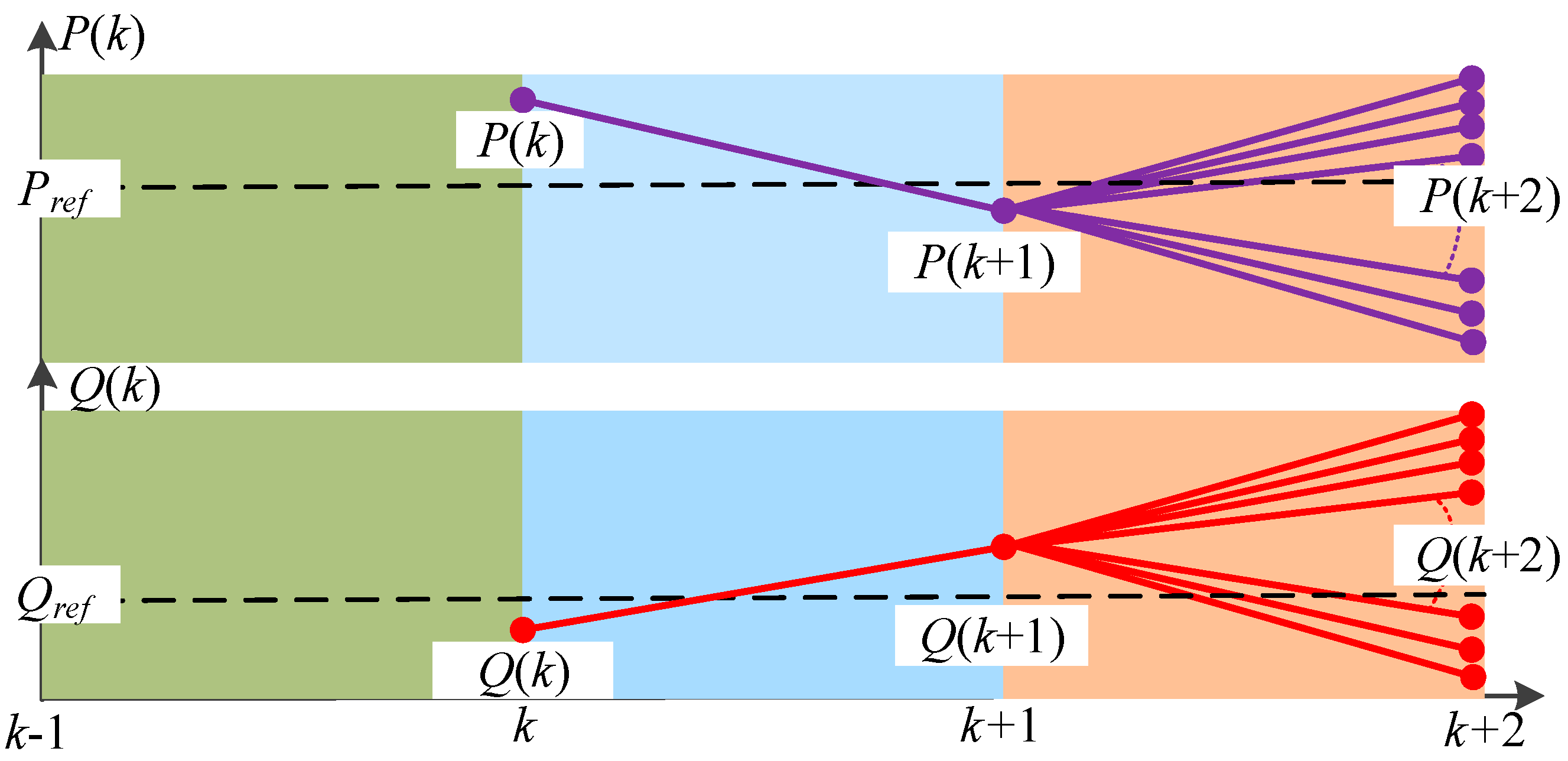
2.3. Conventional OSS-MPC

In conventional OSS-MPC, there are three voltage vectors in one sampling period. Hence, the predicted active and reactive power at instant k + 2 are predicted as
{ P ( k + 2 ) = P ( k + 1 ) + f p 1 ( k + 1 ) t 1 + f p 2 ( k + 1 ) t 2 + f p 3 ( k + 1 ) t 3 Q ( k + 2 ) = Q ( k + 1 ) + f q 1 ( k + 1 ) t 1 + f q 2 ( k + 1 ) t 2 + f q 3 ( k + 1 ) t 3 ,
where fp1(k + 1), fp2(k + 1) and fp3(k + 1) are the derivatives of the active power for two nonzero vectors and one zero vector in one control period, respectively, fq1(k + 1), fq2(k + 1) and fq3(k + 1) are the derivatives of the reactive power similarly. t1, t2 and t3 are the duration time for these vectors. In order to predict P(k + 2) and Q(k + 2), the voltage vectors implemented at instant k should be calculated at instant k − 1.
In reference [31], by setting the dJ/dt to zero, the optimal duration time t1, t2 and t3 can be obtained as
{ t 1 = ( f q 2 f q 3 ) E p + ( f p 3 f p 2 ) E q + ( f p 2 f q 3 f p 3 f q 2 ) T s ( f q 2 f q 3 ) f p 1 + ( f q 3 f q 1 ) f p 2 + ( f q 1 f q 2 ) f p 3 t 2 = ( f q 3 f q 1 ) E p + ( f p 1 f p 3 ) E q + ( f q 1 f p 3 f q 3 f p 1 ) T s ( f q 2 f q 3 ) f p 1 + ( f q 3 f q 1 ) f p 2 + ( f q 1 f q 2 ) f p 3 t 3 = T s t 1 t 2 ,
where fp1, fp2 and fp3 represent fp1(k + 1), fp2(k + 1) and fp3(k + 1), fq1, fq2 and fq3 represent fq1(k + 1), fq2(k + 1) and fq3(k + 1), Ep = PrefP(k + 1), Eq = QrefQ(k + 1).
There are six combinations of the voltage vector sequences for OSS-MPC with two nonzero vectors and one zero vector in one control period. Therefore, through six calculations of Equations (4) and (8)–(11), the optimal switching sequence with minimal cost function J can be obtained. Particularly, the calculation amount of Equation (11) in the six calculations is dramatically large, since there are two division operations. Figure 5 shows the flow diagram of the conventional OSS-MPC.

3. Simplified OSS-MPC

To improve the efficiency of minimizing the cost function, the ideal voltage vector and the center vectors are introduced to reduce the calculation times of Equation (11) from six to one. Analogous to FCS-MPC, the center vectors in the six sectors are applied to minimize the cost function instead of the vector sequences.

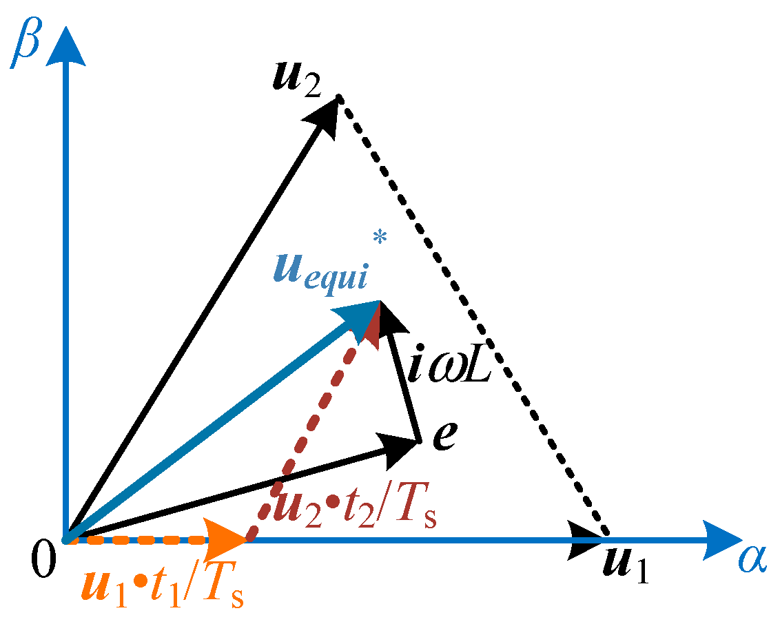
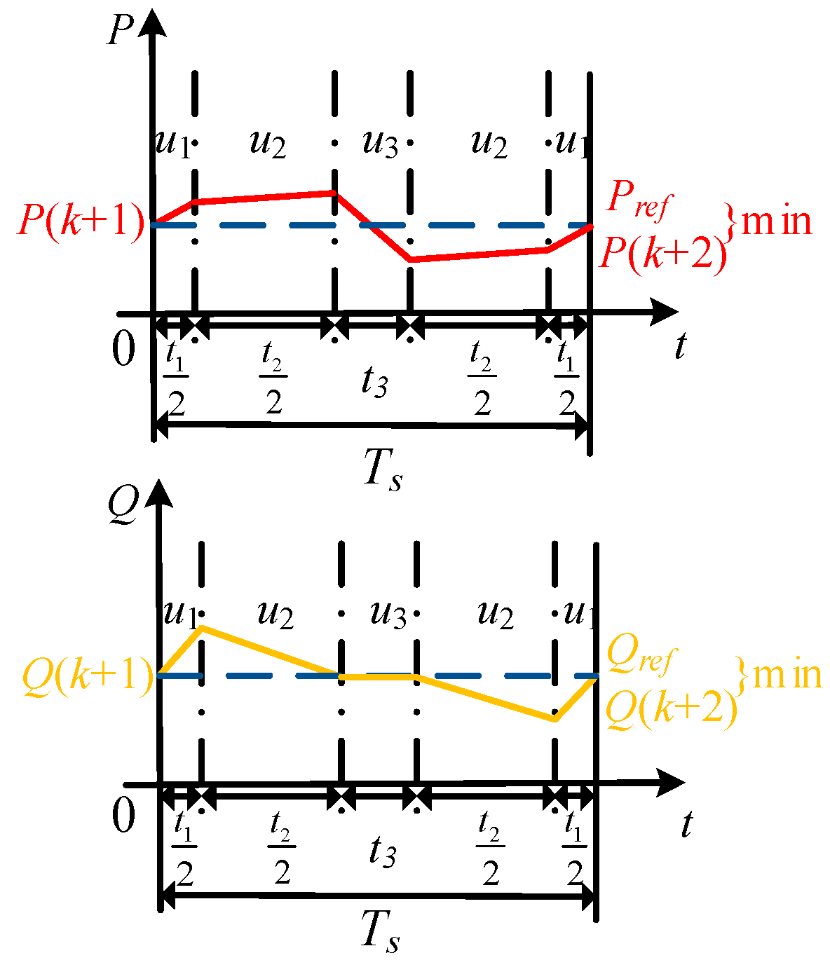
3.1. Equivalent Ideal Voltage Vector of Output Voltage Vector Sequence

Since the gradient of the active and reactive power during the duration of the voltage vector is considered constant, the active and reactive power trajectories during the sampling period are shown as Figure 6. Equation (9), the cost function, can choose the vector sequence that minimizes the deviation between P(k + 2) and Pref.
Therefore, we can use an equivalent ideal voltage to track the reference power. When the ideal voltage vector u*equi that can perfectly track the reference power is located in sector I, u1 and u2 in Figure 2 are selected as the two nonzero voltage vectors of vector sequence. With a zero voltage vector, they can equivalently generate the ideal voltage vector u*equi, as shown in Figure 7.

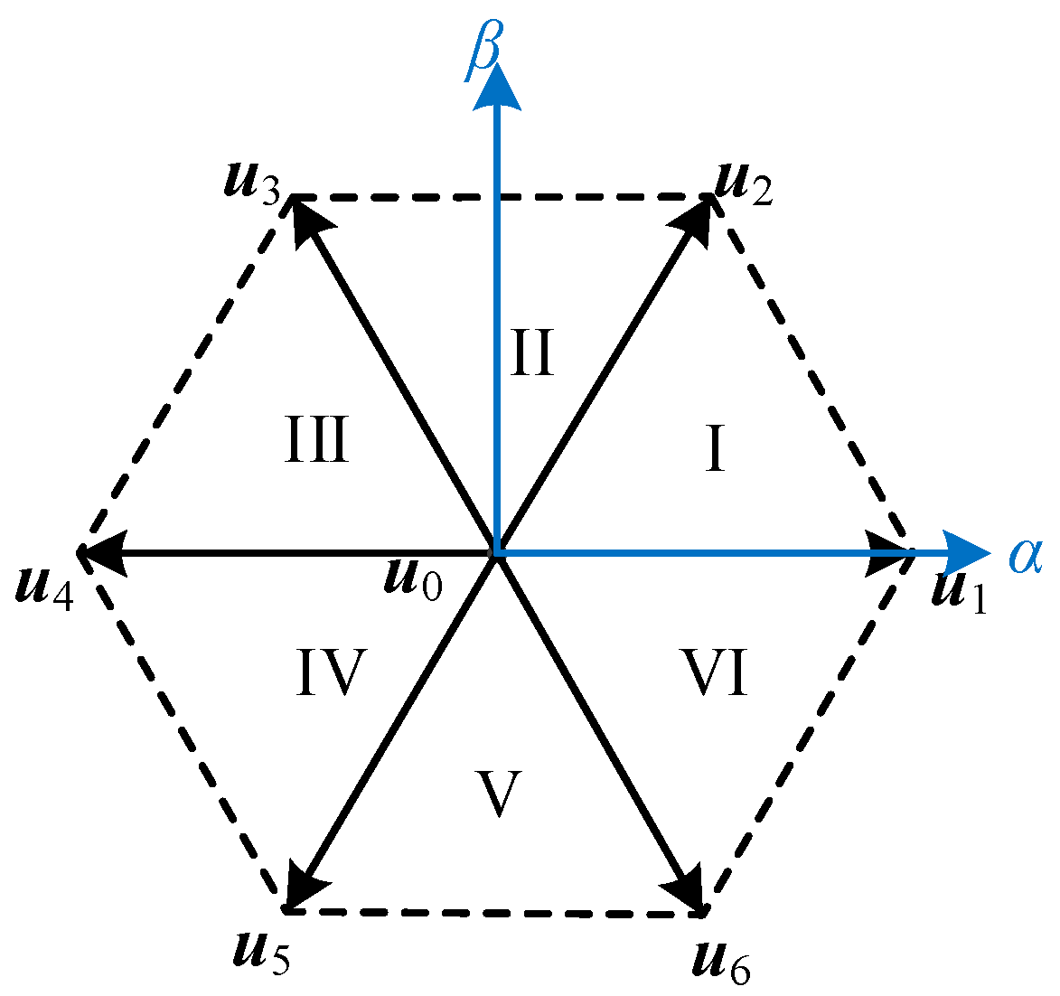
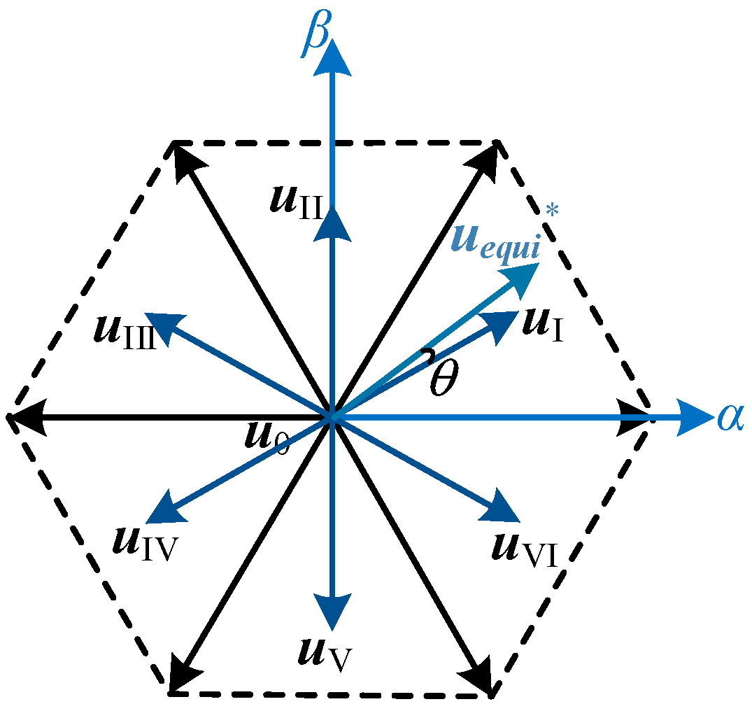
3.2. Center Vectors in Six Sectors

In this section, the concept of the center vector is introduced. The ends of the center vectors are located at the centroids of six triangular sectors, as shown in Figure 8.
In Figure 8, uI, uII, uIII, uIV, uV, uVI are the center vectors of the six sectors, respectively. They are the finite control set (FCS) of the cost function optimization.

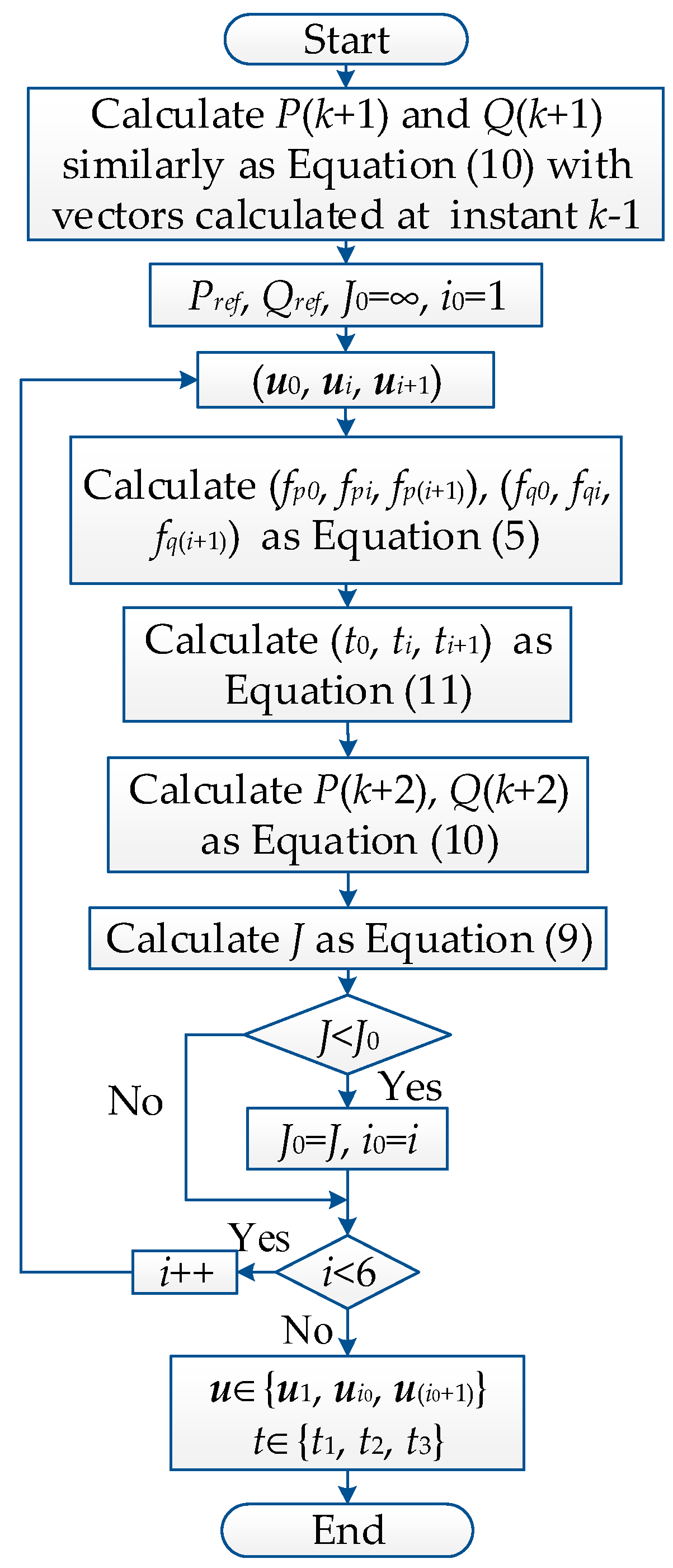
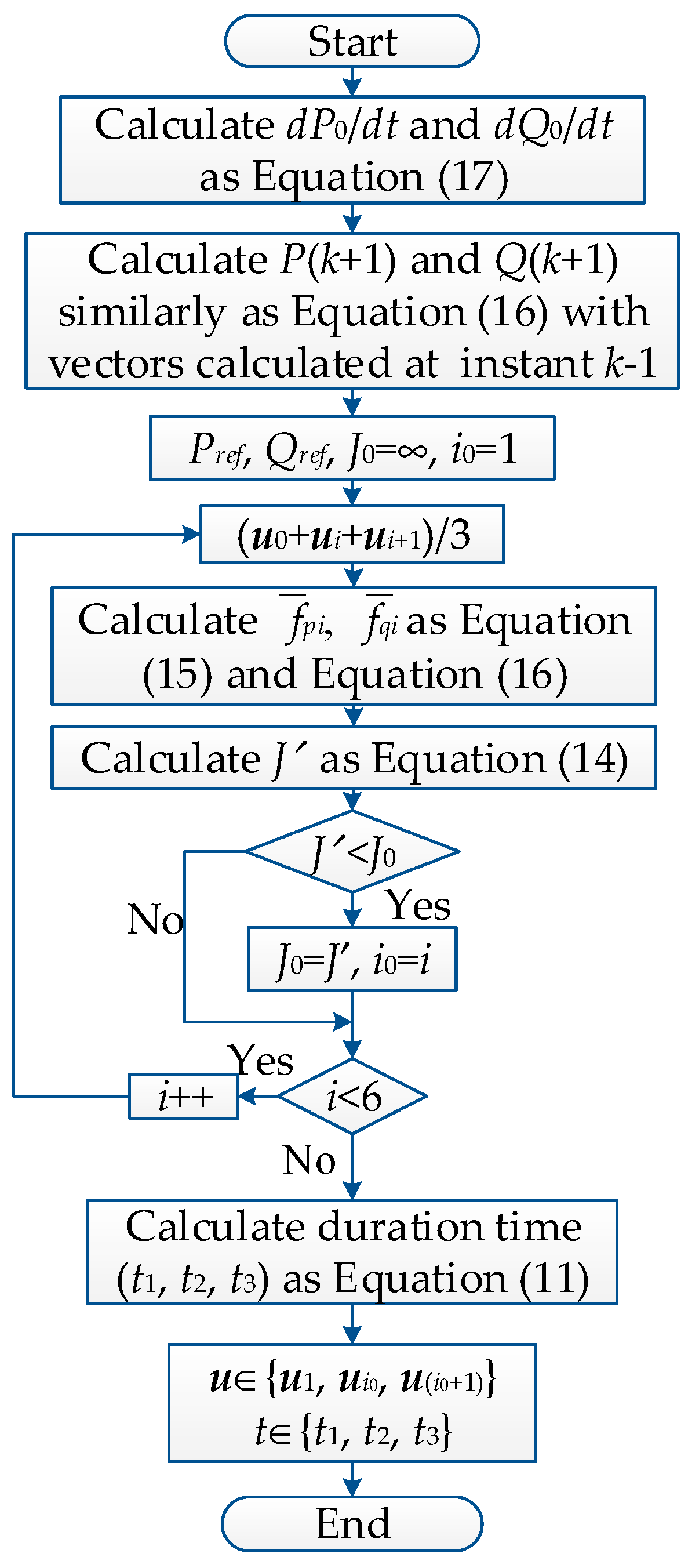
3.3. FCS Moving Horizon Optimization

With the definition of the equivalent ideal voltage vector and center vector, we can use them to improve the efficiency of the moving horizon optimization. Combining Equation (4) with cost function, the cost function to track the reference power can be rewritten as
J = [ f p * T s f p i T s ] 2 + [ f q * T s f q i T s ] 2 = 9 T s 2 ( e α 2 + e β 2 ) l 2 2 L 2 ,
where l is the distance between u*equi and the voltage vectors.
As shown in Figure 8, according to cosine theorem, the square of the distance between u*equi and the six center vectors can be calculated as
l 2 = | u e q u i * | 2 + | u c i | 2 2 | u e q u i * | | u c i | cos θ i = ( u α * u α i ) 2 + ( u β * u β i ) 2 ,
where uci is the center vector, indicating uI, uII, uIII, uIV, uV and uVI.
It can be seen from Equation (13) that the distance l is determined by θ, since |u*equi| and |uci| are constant. If u*equi is located in the sector I as shown in Figure 8, θ gets minimum with uI than the other center vectors. Inspired by FCS-MPC, we can substitute the center vectors into the cost function to find out which sector the ideal voltage vector u*equi is in without calculating the optimal duration time. The cost function to obtain the sector where the ideal voltage vector u*equi is located is
J = [ P r e f P ( k + 1 ) f ¯ p i T s ] 2 + [ Q r e f Q ( k + 1 ) f ¯ q i T s ] 2 ,
where
{ f ¯ p i = d P i d t f ¯ q i = d Q i d t | u c i = u 0 + u i + u i + 1 3 .
Assuming that the ideal voltage vector u*equi is as shown in Figure 8. Then uI in FCS will be chosen as the center vector that minimizes the cost function J′. According to the above analysis, vector sequence (u0, u1, u2) will be selected as the optimal switching sequence. After that, the duration time (t0, t1, t2) for (u0, u1, u2) will be calculated. In this way, we can avoid the duration time calculation in minimizing the cost function. The FCS moving horizon optimization is the core idea of the simplified OSS-MPC.

3.4. Further Reduce the Computational Expense

Based on FCS moving horizon optimization of simplified OSS-MPC, we can further reduce the computational expense by rewriting the Equation (4) as
{ d P d t = 3 2 ( e α u α i L + e β u β i L + d P 0 d t ) d Q d t = 3 2 ( e β u α i L e α u β i L + d Q 0 d t ) ,
where dP0/dt and dQ0/dt are the constant term of the derivatives of the active and reactive powers, respectively. They depend on the grid current and grid voltage, which are considered as constant values during the sampling period. The definition of dP0/dt and dQ0/dt can be obtained from Equation (4) as
{ d P 0 d t = e α ( e α L + ω i β ) + e β ( e β L ω i α ) d Q 0 d t = e β ( e α L + ω i β ) e α ( e β L ω i α ) .
According to the above analysis, we can extract the constant term (i.e., dP0/dt and dQ0/dt) of Equation (17) outside the moving horizon optimization. In this way, Equation (17) will not need to be calculated during moving horizon optimization. Since one cycle calculation of P(k + 1), Q(k + 1) and 6 cycle calculations of Equation (16) for the center vectors, the extraction of Equation (17) can save 6 cycle calculations of Equation (17). Meanwhile, this modification of Equation (4) during moving horizon optimization only change the calculation order without changing the calculation results, and will not affect the control performance. The flow diagram of the whole simplified OSS-MPC is shown in Figure 9. During the simplified OSS-MPC, the constant term dP0/dt and dQ0/dt are calculated outside the moving horizon optimization. With delay compensation, P(k + 1) and Q(k + 1) are predicted as Equation (16) with the OSS calculated at instant k − 1. Afterwards, the center vectors are used to select the OSS through FCS moving horizon optimization. Eventually, the OSS is applied to the inverter with the optimal duration time (t1, t2, t3) obtained by Equation (11).
Comparing Figure 9 with Figure 5, the underlying principle of the simplified OSS-MPC is that it uses the switching states to search the optimal switching sequence (OSS) rather than switching sequences directly. Thus, the simplified OSS-MPC only needs to go over all 6 switching states and while the conventional one needs to go over all 6 switching sequences. And using switching sequences means calculating Equation (11) during 6 cycles, while the simplified OSS-MPC only need to calculate Equation (11) once after finding the OSS without containing the duration time.

4. Simulation and Experimental Results

In order to verify the effectiveness of the simplified OSS-MPC, a comparative study with conventional OSS-MPC is carried out. The grid side line voltage 220 V is obtained by the Y/Δ isolation transformer. The other parameters of the simulation and experimental systems are shown in Table 1.

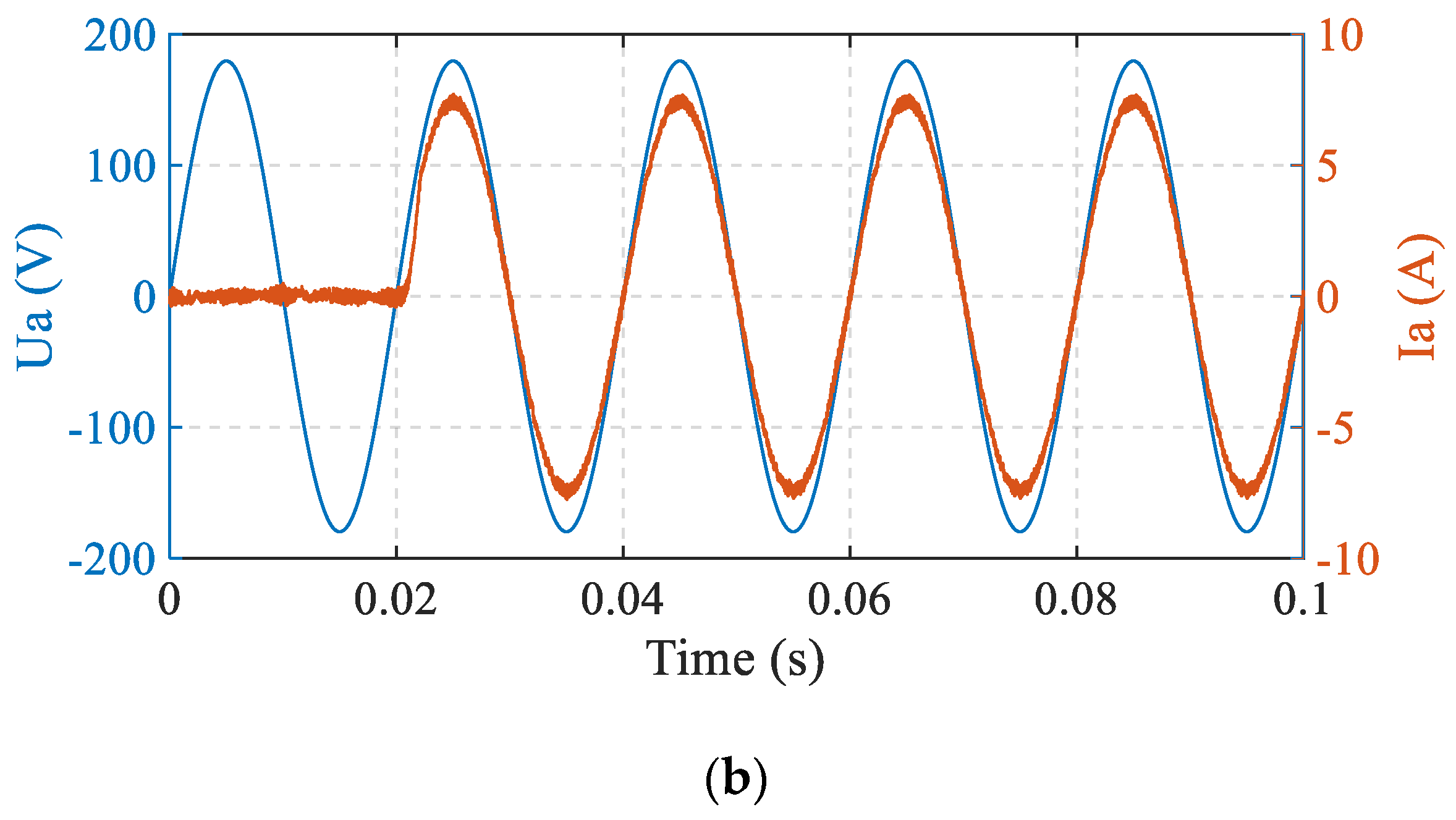
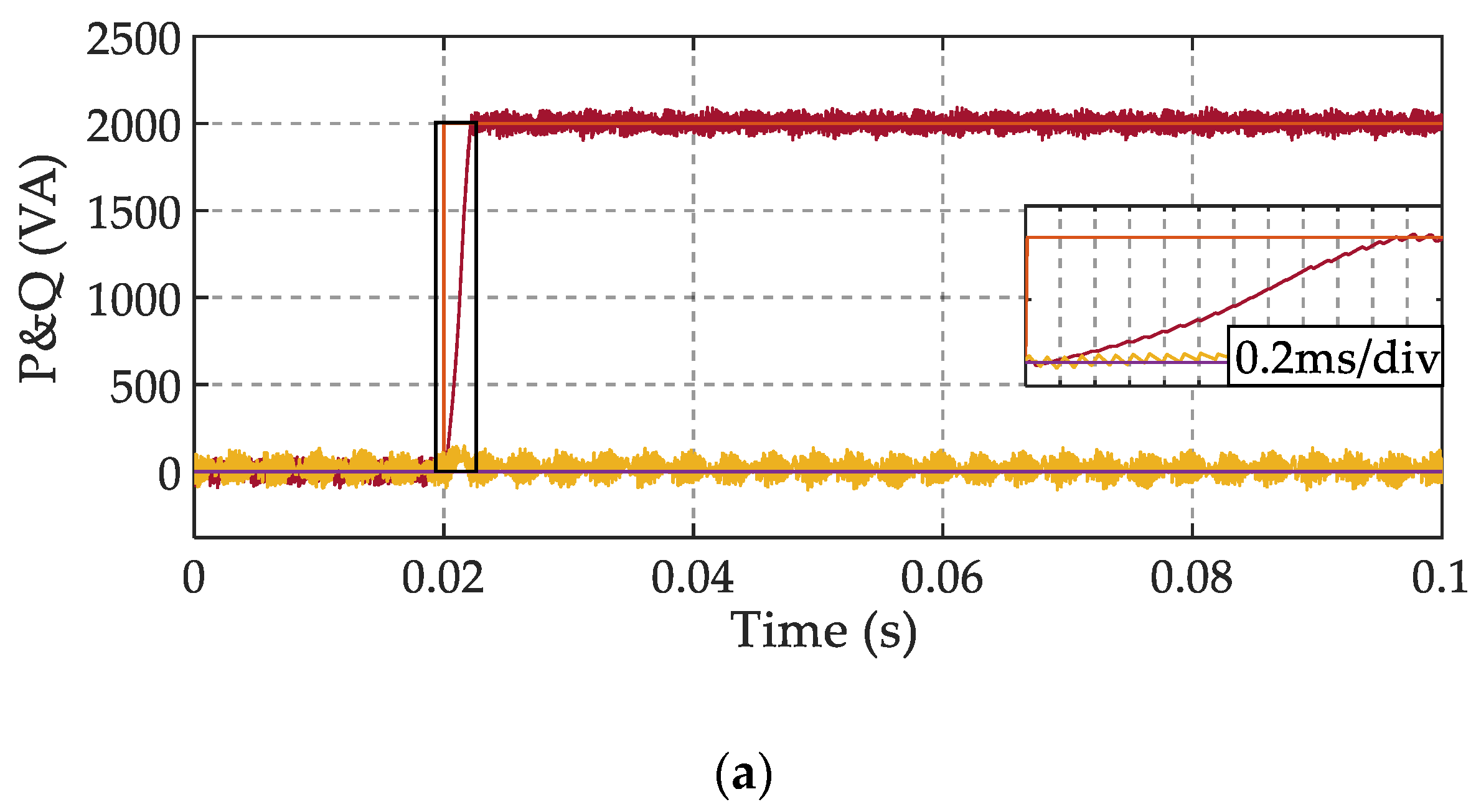
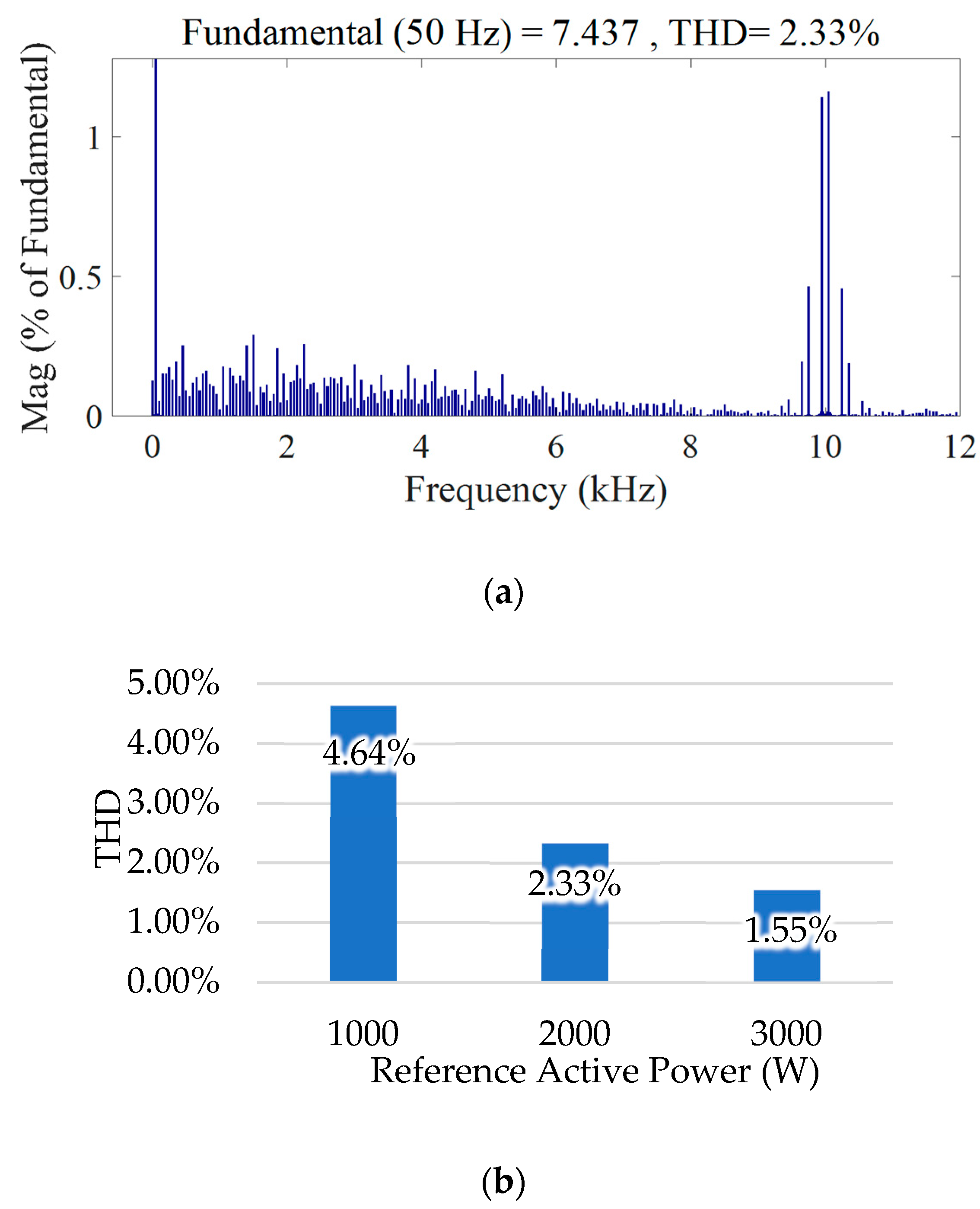
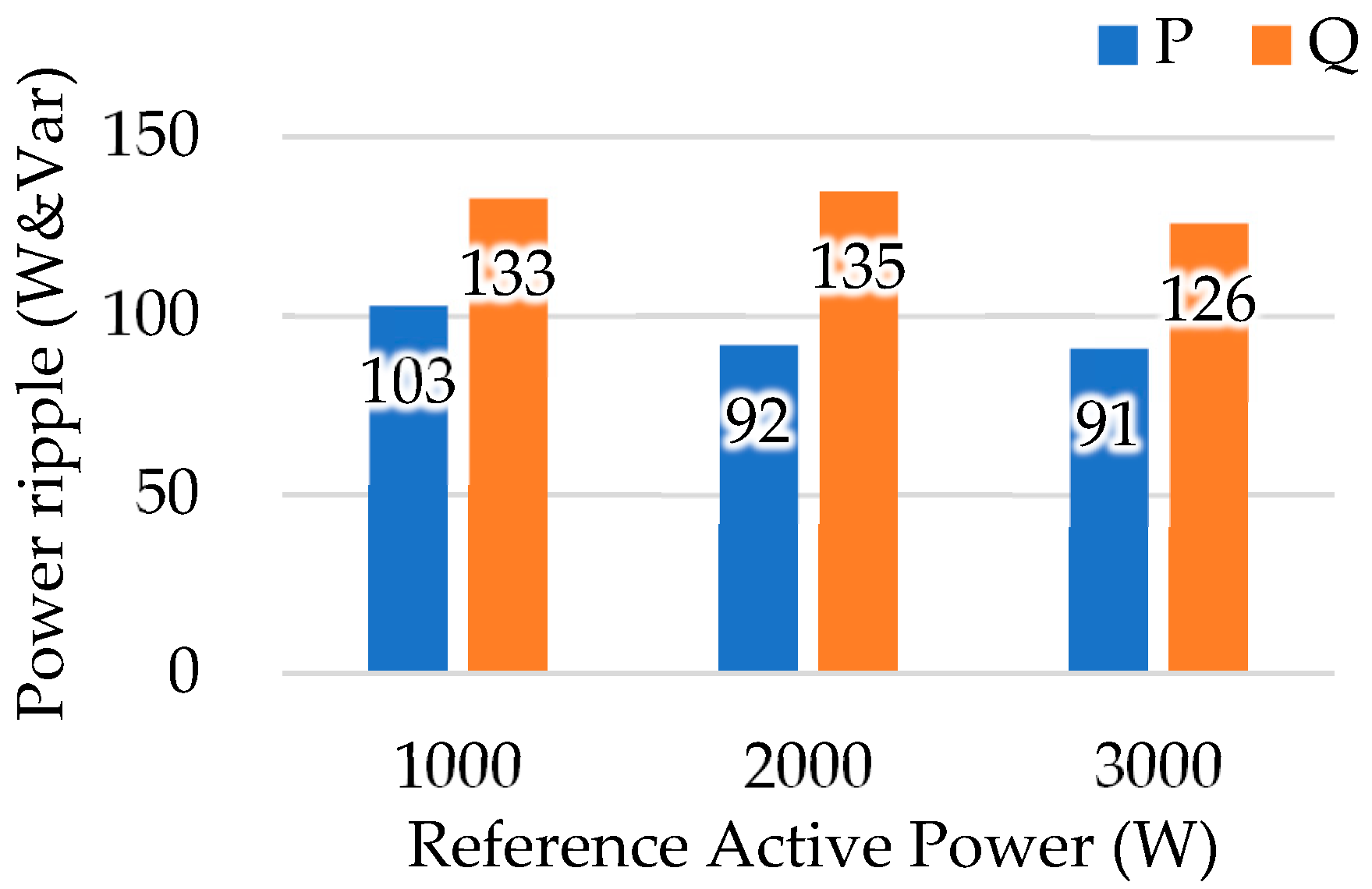
4.1. Simulation Results

Both simplified OSS-MPC and conventional OSS-MPC strategy are simulated in the environment of MATLAB/Simulink. The active power reference steps from 0 to 2000 W at 0.02 s. Meanwhile, the reactive power reference is held at 0 to achieve unity power factor. The proposed algorithm not only reduces the computational burden but also completely maintains the original excellent dynamic and steady-state response of conventional OSS-MPC. The minimum value of J is always equal to 0 during the steady-state, since the output voltage vector sequence has the same effect as the ideal voltage vector at instant k + 2. During each sampling period, both algorithms choose the same voltage vector sequence, and the calculated optimal duration time is the same. Since these two algorithms have the same simulation results, only one of them is shown below.
The dynamic simulation results of the system are presented in Figure 10. Figure 10 illustrates that the proposed algorithm has fast dynamic response, which only needs 2.2 ms to track the reference active power as shown in Figure 10a.
Meanwhile, both algorithms express excellent steady-state performance after the step change. The harmonic content of the output current is presented in Figure 11. The corresponding total harmonic distortion (THD) of phase A output current in steady-state is only 2.33% when the reference active power is 2000 W. It should be noticed that the current harmonics is mainly concentrated at the sampling frequency of 10 kHz. Figure 11b presents the harmonic content of the output current at various operating points, which have very low THD from 1000 W to 3000 W.
The active and reactive power ripple of the simplified OSS-MPC and conventional OSS-MPC are depicted in Figure 12 under various reference active power. Figure 10, Figure 11 and Figure 12 indicate that the proposed algorithm maintains the high performance of the conventional OSS-MPC during transient and steady states.

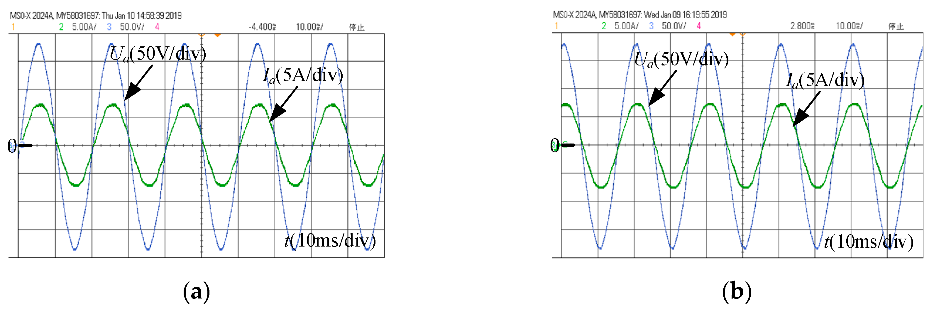
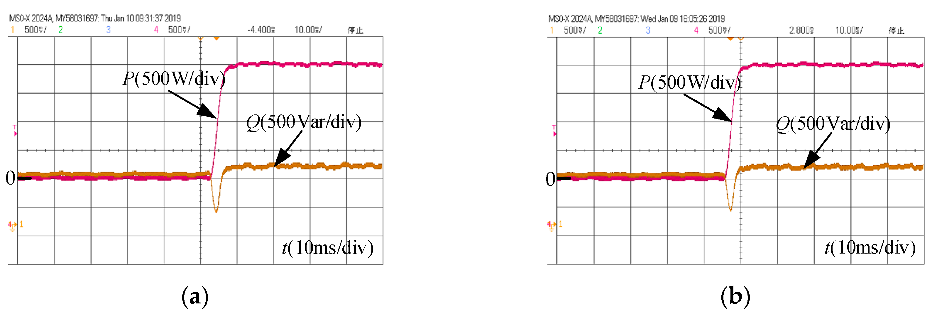
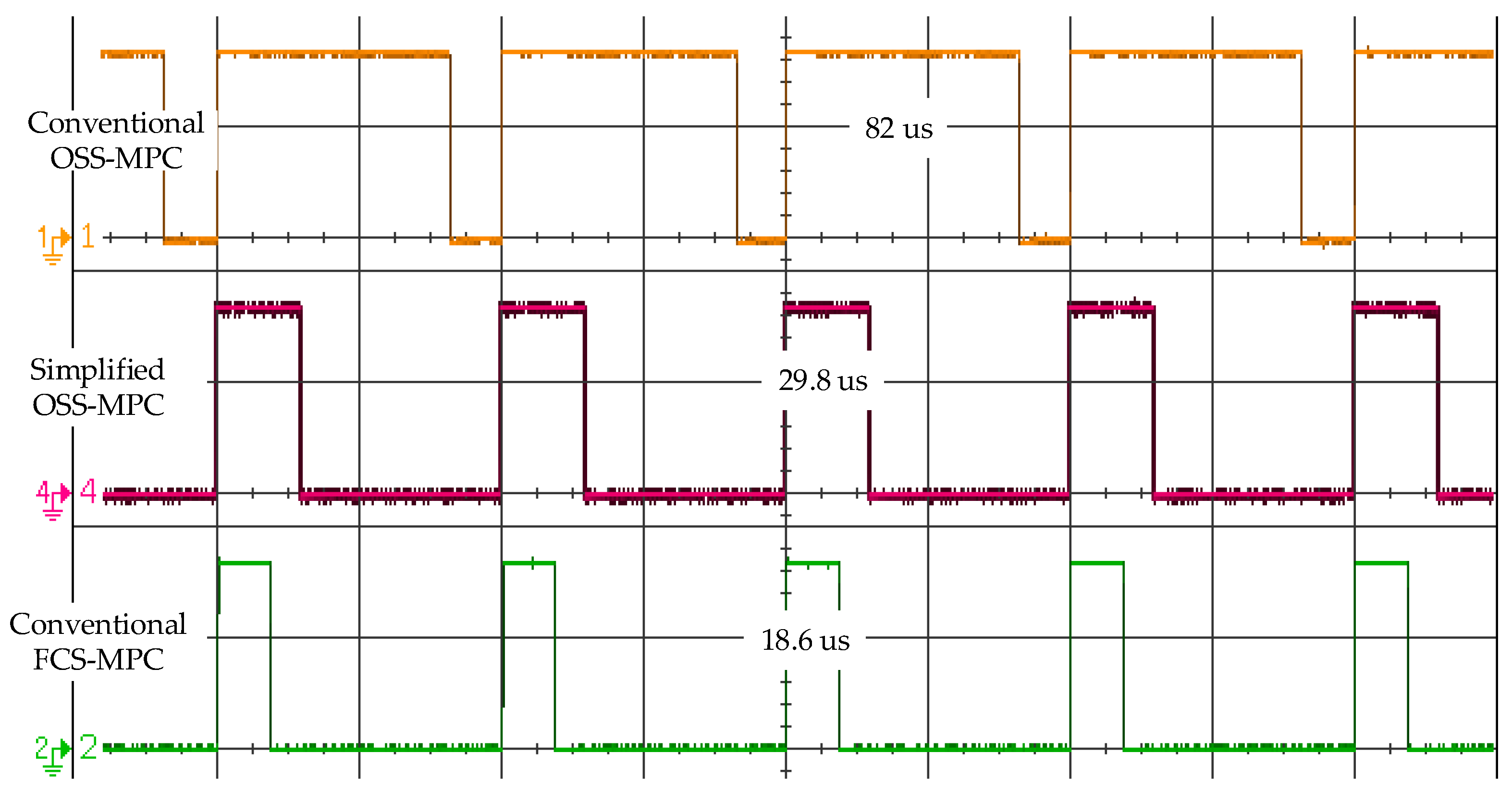
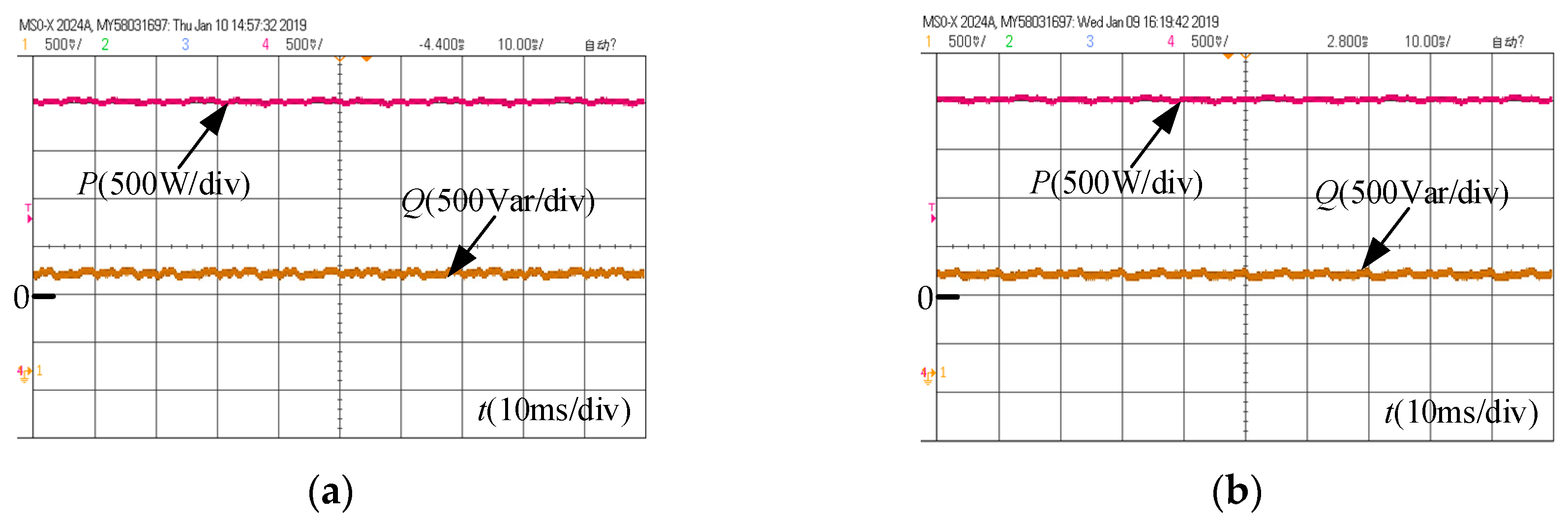
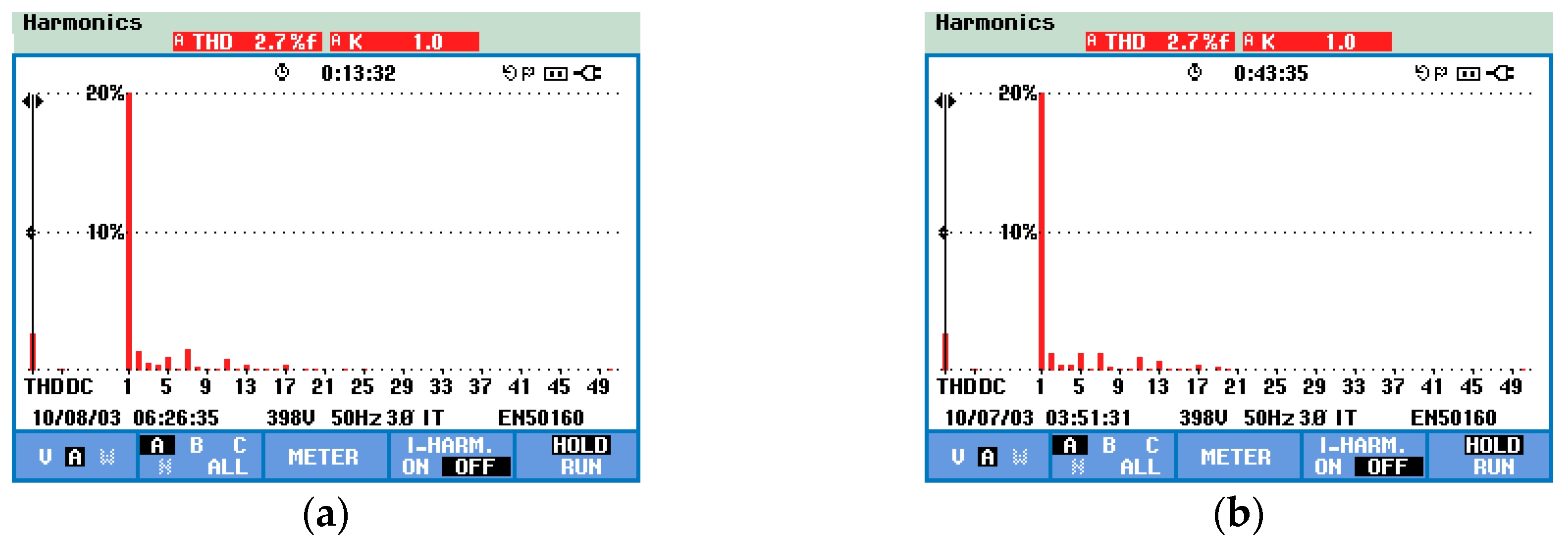
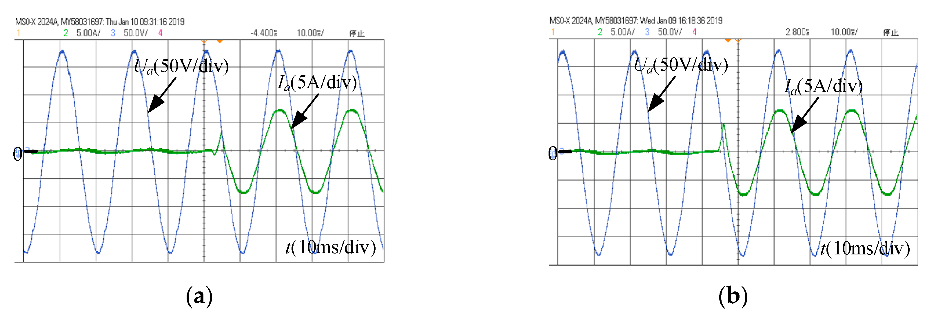
4.2. Experimental Results

The experimental control board is based on a 32 bit 150MHz DSP (TMS320F28335). The insulated gate bipolar transistors (IGBTs) used are IKW50N60T, and the dead time is set to 3μs. The output current spectrum is measured by the power quality analyzer Fluke435.
First of all, we measured the execution time of the conventional OSS-MPC and simplified OSS-MPC. As shown in Figure 13, the execution time of conventional FCS-MPC was 18.6us. However, it cannot achieve constant switching frequency. At the same time, the conventional OSS-MPC requires 82 μs execution time, while the simplified OSS-MPC only needs 29.8 μs. For one thing, the shorter execution time enables the inverter to enhance the switching frequency or to extend prediction horizons (with more than one prediction step), which can improve the steady-state performance. For another, we can use the spare time to implement other functions in renewable energy sources, such as islanding detection protection or maximum power point tracking of the wind turbine system.
Figure 14 and Figure 15 show the steady-state experimental results of the conventional OSS-MPC and simplified OSS-MPC. The active power is set to 2000 W while the reactive power is set to 0 Var. Figure 14a,b depict the steady-state waveforms of the active and reactive power under conventional OSS-MPC and the simplified OSS-MPC, respectively. Figure 15 shows the steady-state waveforms of grid voltage and current. The steady-state experimental results show that both control strategies can track the power reference accurately. Additionally, both control strategies have the same low THD as shown in Figure 16.
To further validate the dynamic performance, the active power is stepped from 0 W to 2000 W while the reactive power maintains 0 Var. Figure 17a,b presents the transient waveforms of the active and reactive power under conventional OSS-MPC and simplified OSS, respectively. Figure 18a,b presents the transient waveforms of grid voltage and current under conventional OSS-MPC and simplified OSS-MPC, respectively. Since the experiment has different trigger phase angle with simulation, the transient waveforms are slightly different from the simulation results in Figure 10. However, Figure 17 and Figure 18 illustrate that the simplified OSS-MPC has the same fast dynamic performance with conventional OSS-MPC, which can track the reference active power within 5 ms as shown in Figure 17.

5. Conclusions

In order to improve the computation efficiency of OSS-MPC, this paper proposes a simplified OSS-MPC strategy for a grid-connected inverter. The simplified OSS-MPC improves moving horizon optimization by introducing the ideal voltage vector and the center vectors, which is similar to FCS-MPC. Besides, the equation structure of the derivatives of the active and reactive powers is modified to further reduce the computational expense.
As the simulation and experiment results show, the execution time of the simplified OSS-MPC is reduced by 63.7% compared to conventional OSS-MPC. Simultaneously, the proposed algorithm maintains the superb performance of the OSS-MPC, which not only has a low power ripple and current THD, but also a very fast dynamic response. Therefore, the simplified OSS-MPC has a good application prospect in industrial applications with a low-cost microprocessor.
In addition, the proposed algorithm is conducive to achieving the longer prediction horizons, and its extension to systems with additional levels is also under study.

Author Contributions

All authors contributed to this work by collaboration. conceptualization, L.K. and J.C.; methodology, B.H.; software, J.C.; validation, B.H., J.C.; formal analysis, J.C.; investigation, B.H.; resources, L.K.; data curation, X.L.; writing—original draft preparation, J.C.; writing—review and editing, X.L. and J.Z.; project administration, L.K.; funding acquisition, L.K.

Funding

This research was funded by Science and Technology Development Special Foundation of Guangdong, China (2017B010120001).

Acknowledgments

I would like to give my sincere gratitude to Longyun Kang, my tutor who gave me great help during the experiments and the paper-writing.

Conflicts of Interest

The authors declare no conflict of interest.

Nomenclature

MPCModel predictive control
OSS-MPCOptimal-switching-sequence model-predictive-control
CCS-MPCContinuous-control-set model-predictive-control
FCS-MPCFinite-control-set model-predictive-control
DSPDigital signal processor
VOCVoltage oriented control
PIcontroller Proportional integral controller
DPCDirect power control
DTCDirect torque control
P-DPCPredictive direct power control
SVMSpace vector modulation
D-MPCDual vector based model-predictive-control
ROSS-DPCReduced optimal-switching-sequence direct power control
IGBTInsulated gate bipolar transistor
eGrid voltage
VdcDirect current power supply
LInductance of AC filter
C1, C2Dc-link capacitors
SX1, SX2Upper and lower switching states of each phase
ui (u0, u1, u2, u3, u4, u5, u6)Output voltage vector of switching state
iGrid current vector
^Complex conjugate
SApparent power
PActive power
QReactive power
MPPCModel predictive power control
MPCCModel predictive current control
ωGrid angular frequency
fpi, fqiDerivatives of active and reactive power
TsSampling period
tdelayDelay time between sampling instant and implementation
JCost function
t1, t2, t3Optimal duration time of optimal switching sequence
uci (uI, uII, uIII, uIV, uV, uVI)Center vector
u*equiIdeal voltage vector
lDistance between u*equi and center vector
JCost function to obtain the sector where ideal voltage vector u*equi is located
f ¯ p i , f ¯ q i Derivatives of active and reactive power of center vector
dP0/dt, dQ0/dtConstant term of derivatives of active and reactive power
fLine voltage frequency
fsSampling frequency
THDTotal harmonic distortion

References

  1. Cheng, C.; Nian, H.; Wang, X.; Sun, D. Dead-beat predictive direct power control of voltage source inverters with optimised switching patterns. IET power Electron. 2017, 10, 1438–1451. [Google Scholar] [CrossRef]
  2. Song, Z.; Tian, Y.; Chen, W.; Zou, Z.; Chen, Z. Predictive Duty Cycle Control of Three-Phase Active-Front-End Rectifiers. IEEE Tran. Power Electron. 2016, 31, 698–710. [Google Scholar] [CrossRef]
  3. Blasko, V.; Kaura, V. A new mathematical model and control of a three-phase AC-DC voltage source converter. IEEE Trans. Power Electron. 1997, 12, 116–123. [Google Scholar] [CrossRef]
  4. Malinowski, M.; Kazmierkowski, M.P.; Hansen, S.; Blaabjerg, F.; Marques, G.D. Virtual-Flux-Based Direct Power Control of Three-Phase PWM Rectifiers. IEEE Trans. Ind. Appl. 2001, 37, 1019–1027. [Google Scholar] [CrossRef]
  5. Noguchi, T.; Tomiki, H.; Kondo, S.; Takahashi, I. Direct power control of PWM converter without power-source voltage sensors. IEEE Trans. Ind. Appl. 1998, 34, 473–479. [Google Scholar] [CrossRef]
  6. Young, H.A.; Perez, M.A.; Rodriguez, J.; Abu-Rub, H. Assessing Finite-Control-Set Model Predictive Control: A Comparison with a Linear Current Controller in Two-Level Voltage Source Inverters. IEEE Ind. Electron. 2014, 8, 44–52. [Google Scholar] [CrossRef]
  7. Kouro, S.; Cortes, P.; Vargas, R.; Ammann, U.; Rodriguez, J. Model Predictive Control—A Simple and Powerful Method to Control Power Inverters. IEEE Trans. Ind. Electron. 2009, 56, 1826–1838. [Google Scholar] [CrossRef]
  8. Dragičević, T. Model Predictive Control of Power Inverters for Robust and Fast Operation of AC Microgrids. IEEE Trans. Power Electron. 2018, 33, 6304–6317. [Google Scholar] [CrossRef]
  9. Panten, N.; Hoffmann, N.; Fuchs, F.W. Finite Control Set Model Predictive Current Control for Grid-Connected Voltage-Source Inverters with LCL Filters: A Study Based on Different State Feedbacks. IEEE Trans. Power Electron 2016, 31, 5189–5200. [Google Scholar] [CrossRef]
  10. Zhang, Y.; Peng, Y.; Yang, H. Performance Improvement of Two-Vectors-Based Model Predictive Control of PWM Rectifier. IEEE Trans. Power Electron 2016, 31, 6016–6030. [Google Scholar] [CrossRef]
  11. Nikhil, P.; Sonam, K.; Monika, M.; Wagh, S. Finite control set model predictive control for two level inverter with fixed switching frequency. In Proceedings of the 2018 SICE International Symposium on Control Systems (SICE ISCS), Tokyo, Japan, 9–11 March 2018; pp. 74–81. [Google Scholar]
  12. Donoso, F.; Mora, A.; Cardenas, R.; Angulo-Cárdenas, A.; Sáez, D. Finite-Set Model Predictive Control Strategies for a 3L-NPC Inverter Operating with Fixed Switching Frequency. IEEE Trans. Ind. Electron. 2018, 65, 3954–3965. [Google Scholar] [CrossRef]
  13. Hu, J. Improved Dead-Beat Predictive DPC Strategy of Grid-Connected DC–AC Inverters with Switching Loss Minimization and Delay Compensations. IEEE Trans. Ind. Inf. 2013, 9, 728–738. [Google Scholar] [CrossRef]
  14. Hu, J.; Zhu, Z.Q. Improved Voltage-Vector Sequences on Dead-Beat Predictive Direct Power Control of Reversible Three-Phase Grid-Connected Voltage-Source Inverters. IEEE Trans. Power Electron. 2013, 28, 254–267. [Google Scholar] [CrossRef]
  15. Vazquez, S.; Marquez, A.; Aguilera, R.; Quevedo, D. Predictive Optimal Switching Sequence Direct Power Control for Grid-Connected Power Inverters. IEEE Trans. Ind. Electron. 2015, 62, 2010–2020. [Google Scholar] [CrossRef]
  16. Tarisciotti, L.; Zanchetta, P.; Watson, A.; Bifaretti, S.; Clare, J.C. Modulated Model Predictive Control for a Seven-Level Cascaded H-Bridge Back-to-Back Inverter. IEEE Trans. Ind. Electron. 2014, 61, 5375–5383. [Google Scholar] [CrossRef]
  17. Tarisciotti, L.; Zanchetta, P.; Watson, A.; Clare, J.C.; Degano, M.; Bifaretti, S. Modulated Model Predictive Control for a Three-Phase Active Rectifier. IEEE Trans. Ind. Appl. 2015, 51, 1610–1620. [Google Scholar] [CrossRef]
  18. Yang, Y.; Wen, H.; Li, D. A Fast and Fixed Switching Frequency Model Predictive Control with Delay Compensation for Three-phase Inverters. IEEE Access. 2017, 5, 17904–17913. [Google Scholar] [CrossRef]
  19. Zhang, Y.; Xie, W.; Li, Z.; Zhang, Y. Low-Complexity Model Predictive Power Control: Double-Vector-Based Approach. IEEE Trans. Ind. Electron. 2014, 61, 5871–5880. [Google Scholar] [CrossRef]
  20. Zhang, Z.; Hackl, C.M.; Kennel, R. Computationally Efficient DMPC for Three-Level NPC Back-to-Back Inverters in Wind Turbine Systems with PMSG. IEEE Trans. Power Electron. 2017, 32, 8018–8034. [Google Scholar] [CrossRef]
  21. Bozorgi, A.M.; Gholami-Khesht, H.; Farasat, M.; Mehraeen, S.; Monfared, M. Model Predictive Direct Power Control of Three-Phase Grid-Connected Inverters with Fuzzy-Based Duty Cycle Modulation. IEEE Trans. Ind. Appl. 2018, 54, 4875–4885. [Google Scholar] [CrossRef]
  22. Yang, Y.; Wen, H.; Fan, M.; Xie, M.; Chen, R. Fast Finite-Switching-State Model Predictive Control Method Without Weighting Factors for T-Type Three-Level Three-Phase Inverters. IEEE Trans. Ind. Inf. 2019, 15, 1298–1310. [Google Scholar] [CrossRef]
  23. Mariethoz, S.; Morari, M. Explicit Model-Predictive Control of a PWM Inverter with an LCL Filter. IEEE Trans. Ind. Electron. 2009, 56, 389–399. [Google Scholar] [CrossRef]
  24. Beccuti, A.G.; Kvasnica, M.; Papafotiou, G.; Morari, M. A Decentralized Explicit Predictive Control Paradigm for Parallelized DC-DC Circuits. IEEE Trans. Control Syst. Technol. 2013, 21, 136–148. [Google Scholar] [CrossRef]
  25. Xia, C.; Tao, L.; Shi, T.; Song, Z. A Simplified Finite-Control-Set Model-Predictive Control for Power Converters. IEEE Trans. Ind. Inf. 2014, 10, 991–1002. [Google Scholar]
  26. Liu, X.; Wang, D.; Peng, Z. Improved finite-control-set model predictive control for active front-end rectifiers with simplified computational approach and on-line parameter identification. ISA Trans. 2017, 69, 51–64. [Google Scholar] [CrossRef]
  27. Kwak, S.; Park, J.C. Switching Strategy Based on Model Predictive Control of VSI to Obtain High Efficiency and Balanced Loss Distribution. IEEE Trans. Power Electron. 2014, 29, 4551–4567. [Google Scholar] [CrossRef]
  28. Rodriguez, J.; Kazmierkowski, M.P.; Espinoza, J.R.; Zanchetta, P.; Abu-Rub, H.; Young, H.A.; Rojas, C.A. State of the Art of Finite Control Set Model Predictive Control in Power Electronics. IEEE Trans. Ind. Inf. 2013, 9, 1003–1016. [Google Scholar] [CrossRef]
  29. Hu, B.; Kang, L.; Cheng, J.; Zhang, Z.; Zhang, J.; Luo, X. Double-step model predictive direct power control with delay compensation for three-level converter. IET Power Electron. 2019, 12, 899–906. [Google Scholar] [CrossRef]
  30. Ngo, V.-Q.-B.; Nguyen, M.-K.; Tran, T.-T.; Choi, J.-H.; Lim, Y.-C. A Modified Model Predictive Power Control for Grid-Connected T-Type Inverter with Reduced Computational Complexity. Electronics 2019, 8, 217. [Google Scholar] [CrossRef]
  31. Aguilera, R.P.; Quevedo, D.E.; Vazquez, S.; Franquelo, L.G. Generalized Predictive Direct Power Control for AC/DC converters. In Proceedings of the IEEE ECCE Asia Downunder (ECCE Asia), Melbourne, VIC, Australia, 3–6 June 2013; pp. 1215–1220. [Google Scholar]
Figure 1. The topology of two-level grid-connected inverter.
Electronics 08 00457 g001
Figure 2. Space vector diagram of the two-level inverter.
Electronics 08 00457 g002
Figure 3. Flow chart of model-predictive-control (MPC).
Electronics 08 00457 g003
Figure 4. Control delay compensation based on the two steps ahead prediction in finite-control-set (FCS)-MPC.
Electronics 08 00457 g004
Figure 5. Flow diagram of the conventional optimal-switching-sequence (OSS)-MPC.
Electronics 08 00457 g005
Figure 6. Active and reactive power trajectories within one sampling period.
Electronics 08 00457 g006
Figure 7. Equivalent ideal voltage vector of output vector sequence.
Electronics 08 00457 g007
Figure 8. Center vectors in six sectors.
Electronics 08 00457 g008
Figure 9. Flow diagram of simplified OSS-MPC.
Electronics 08 00457 g009
Figure 10. System response for step change of (a) active and reactive power; (b) output current.
Electronics 08 00457 g010aElectronics 08 00457 g010b
Figure 11. Harmonic content of the output current at (a) P = 2000 W; (b) various operating points.
Electronics 08 00457 g011
Figure 12. Active and reactive power ripple at various operating points.
Electronics 08 00457 g012
Figure 13. Execution time of conventional OSS-MPC, simplified OSS-MPC, and FCS-MPC.
Electronics 08 00457 g013
Figure 14. Steady-state waveforms of the active and reactive power under (a) conventional OSS-MPC; (b) simplified OSS-MPC.
Electronics 08 00457 g014
Figure 15. Steady-state waveforms of grid voltage and current under (a) conventional OSS-MPC; (b) simplified OSS-MPC.
Electronics 08 00457 g015
Figure 16. Harmonic spectrum of grid current under (a) conventional OSS-MPC; (b) simplified OSS-MPC.
Electronics 08 00457 g016
Figure 17. Transient waveforms of the active and reactive power under (a) conventional OSS-MPC; (b) simplified OSS-MPC.
Electronics 08 00457 g017
Figure 18. Transient waveforms of grid voltage and current under (a) conventional OSS-MPC; (b) simplified OSS-MPC.
Electronics 08 00457 g018
Table 1. Parameters of simulation and experimental system.
System ParameterSymbolValue
Filter inductanceL9 mH
Line voltage frequencyf50 Hz
DC-link capacitorC1, C21000 μF
DC-link voltageUdc350 V
Sampling frequencyfs10 kHz

