Optimal Virtual Machine Placement Based on Grey Wolf Optimization


Abstract
:1. Introduction
- To the best of the authors’ knowledge, this is the first time that GWO has been utilized to address the problem of optimal VM placement; we refer to this method as GWO-VMP. The proposed method reduces the energy consumption of cloud computing by allocating VMs into the minimal number of active PMs.
- The proposed work formulated the VMP optimization problem as discrete and binary GWO problems. The binary approach is more efficient.
- We proposed a method for correcting infeasible solutions (RIS) to accelerate the convergence of the proposed algorithms.
- We performed an extensive experimental study to evaluate the effectiveness and efficiency of the proposed algorithms. The proposed methods performed competitively compared to the state-of-the-art methods.
2. Background and Related Work
2.1. VMP Problem Formulation
2.2. Related Work
2.3. Grey Wolf Optimization
2.4. Binary Grey Wolf
3. GWO for Virtual Machine Placement
3.1. Adjusting GWO for VMP
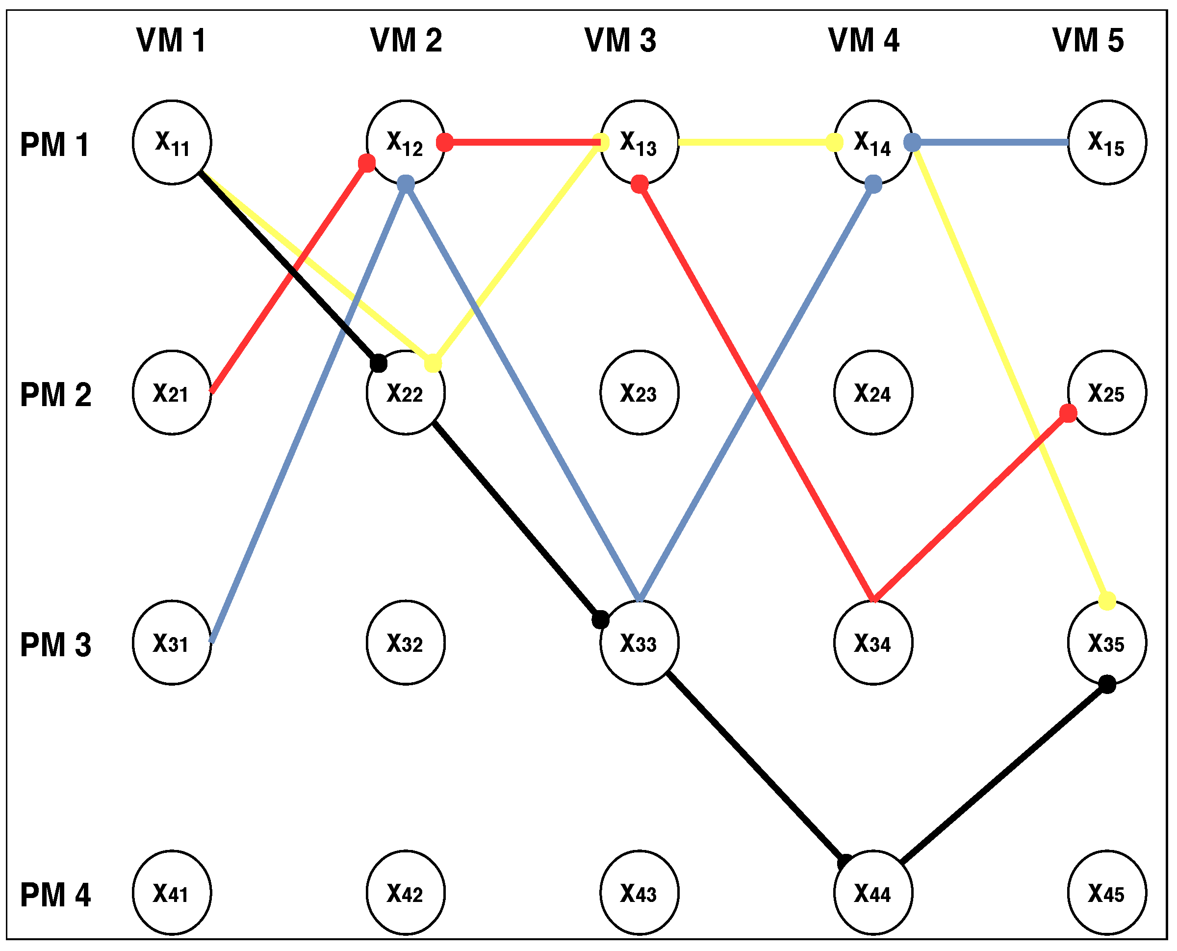
3.2. Solution Construction
3.3. Revising the Infeasible Solutions (RIS)
3.3.1. Eliminating the Duplicate Assignments
3.3.2. Obviating the Overload Assignments
3.3.3. Reassigning the Unallocated VMs
3.4. Objective Function
3.5. BGWO-VMP Algorithm
3.6. DGWO-VMP Algorithm
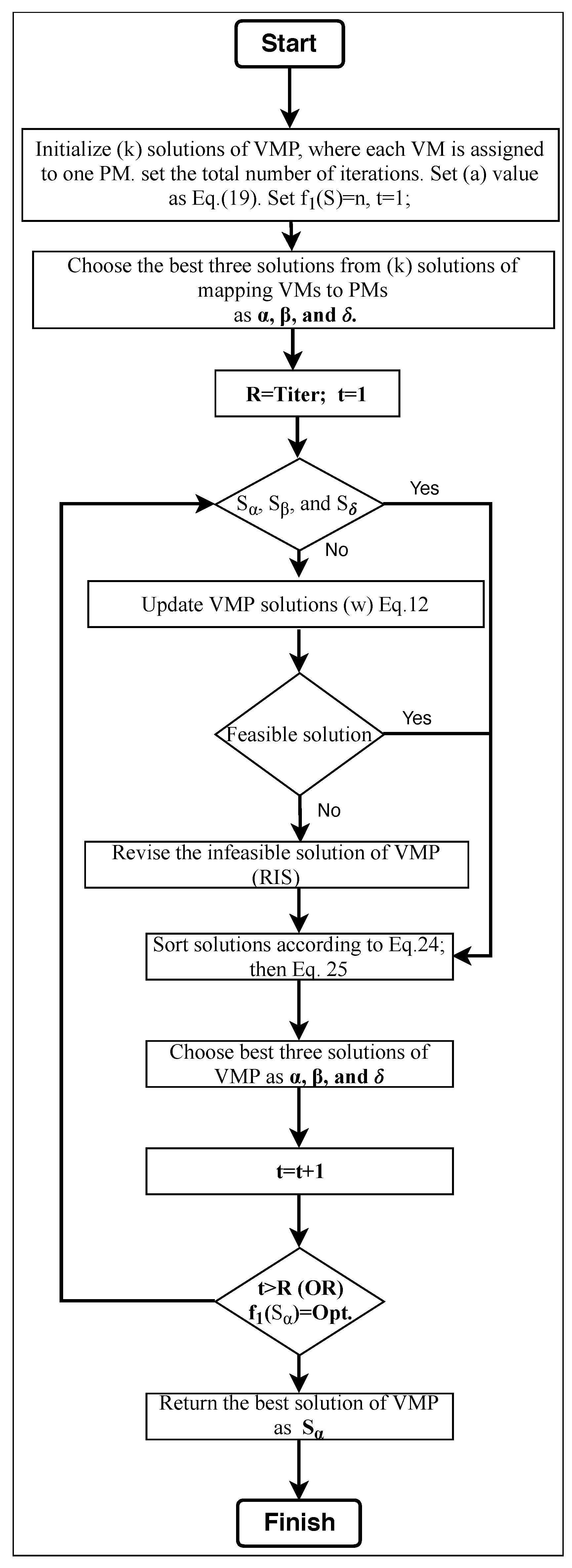
| Algorithm 1: GWO-VMP. |
| Input: the number of VMs, the number of PMs Output: VM allocation map Step 1: Initialization. Set parameter a via Equation (24). Set the number of wolves as k, which are considered as the search agents. Set the total number of iterations and the iteration number . Step 2: Let the k wolves construct the k solutions. Then, select the , , and solutions. Step 3: Update all solutions based on the solutions of , , and and calculate the updated values according to Equation (16) or Equation (27) for the binary and discrete algorithms, respectively. Step 4: Perform RIS if there is an infeasible solution. Step 5: Evaluate the fitness values of the k solutions and identify the best three solutions so far, which are set as , , and for the current iteration. Step 6: Termination detection. If the current iteration number exceeds the maximum number of iterations or the number of active PMs equals the preset optimal number of active PMs, then the algorithm terminates. Otherwise, increase by 1 and return to step (3) for the next iteration. Step 7: Return a solution as the best solution. |
4. Experiment and Comparisons
4.1. Bottleneck of a Resource Homogeneous Environment
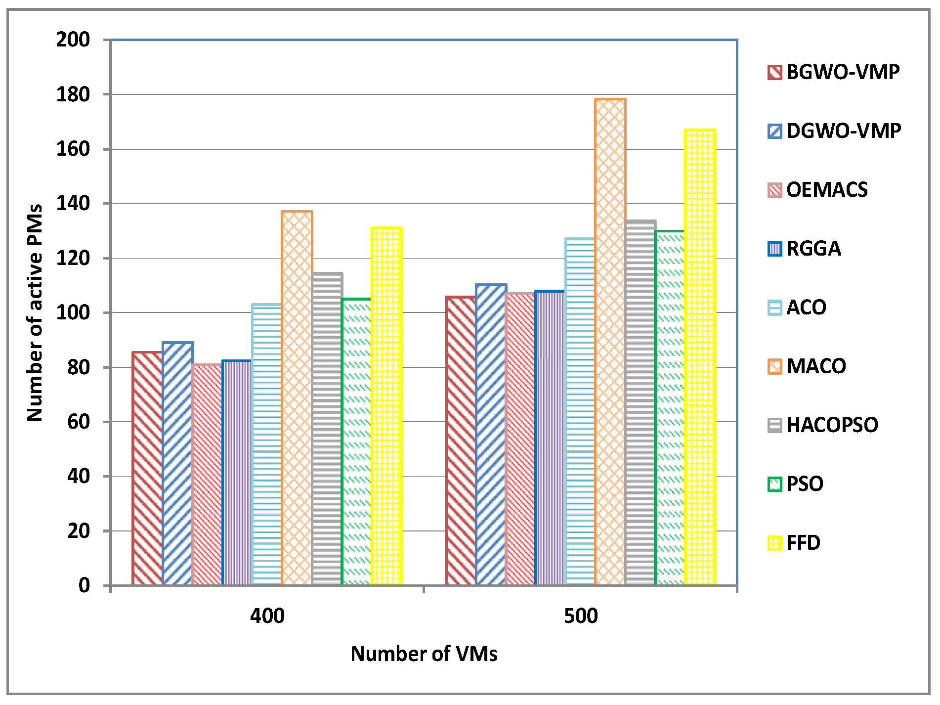
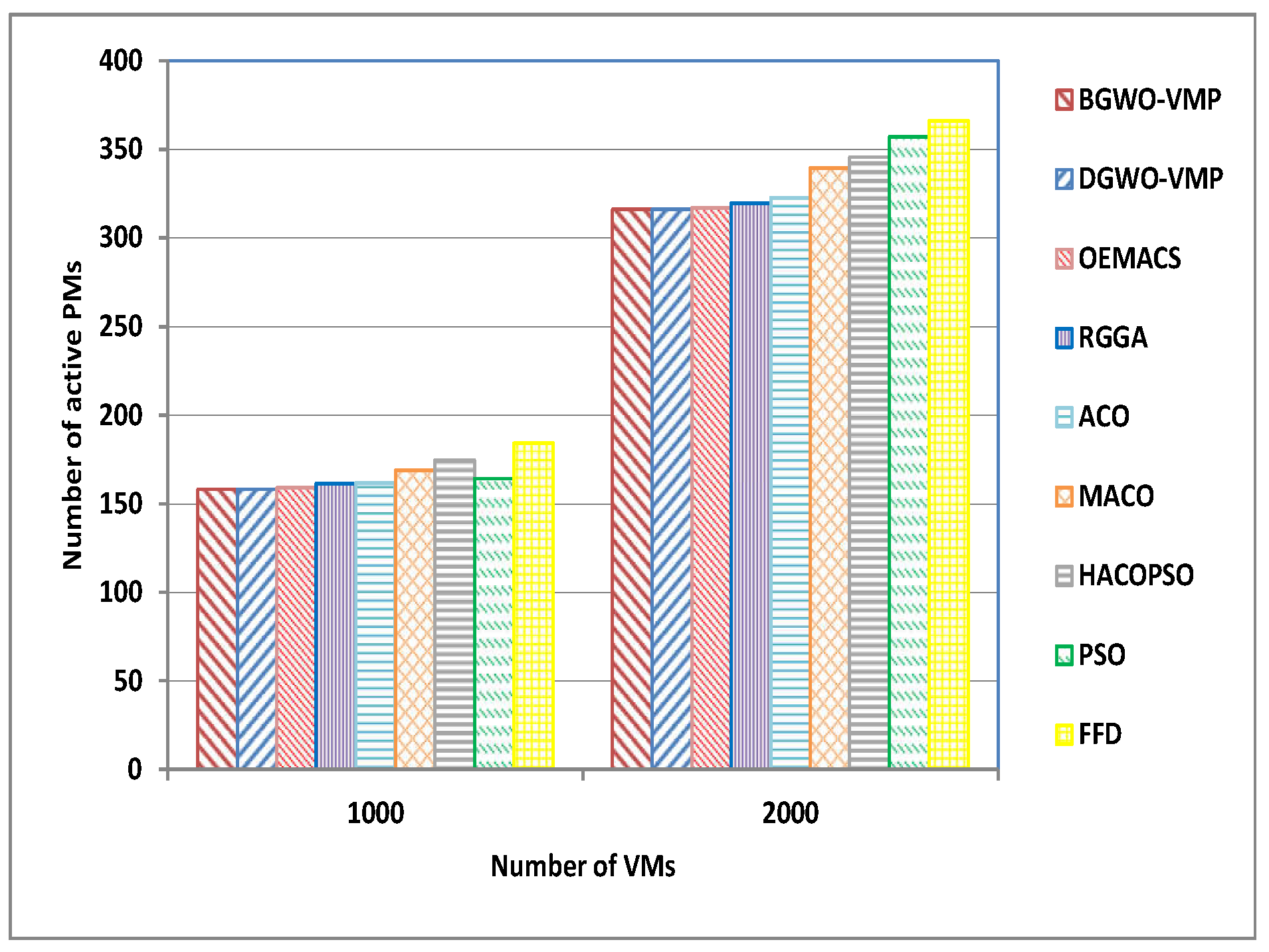
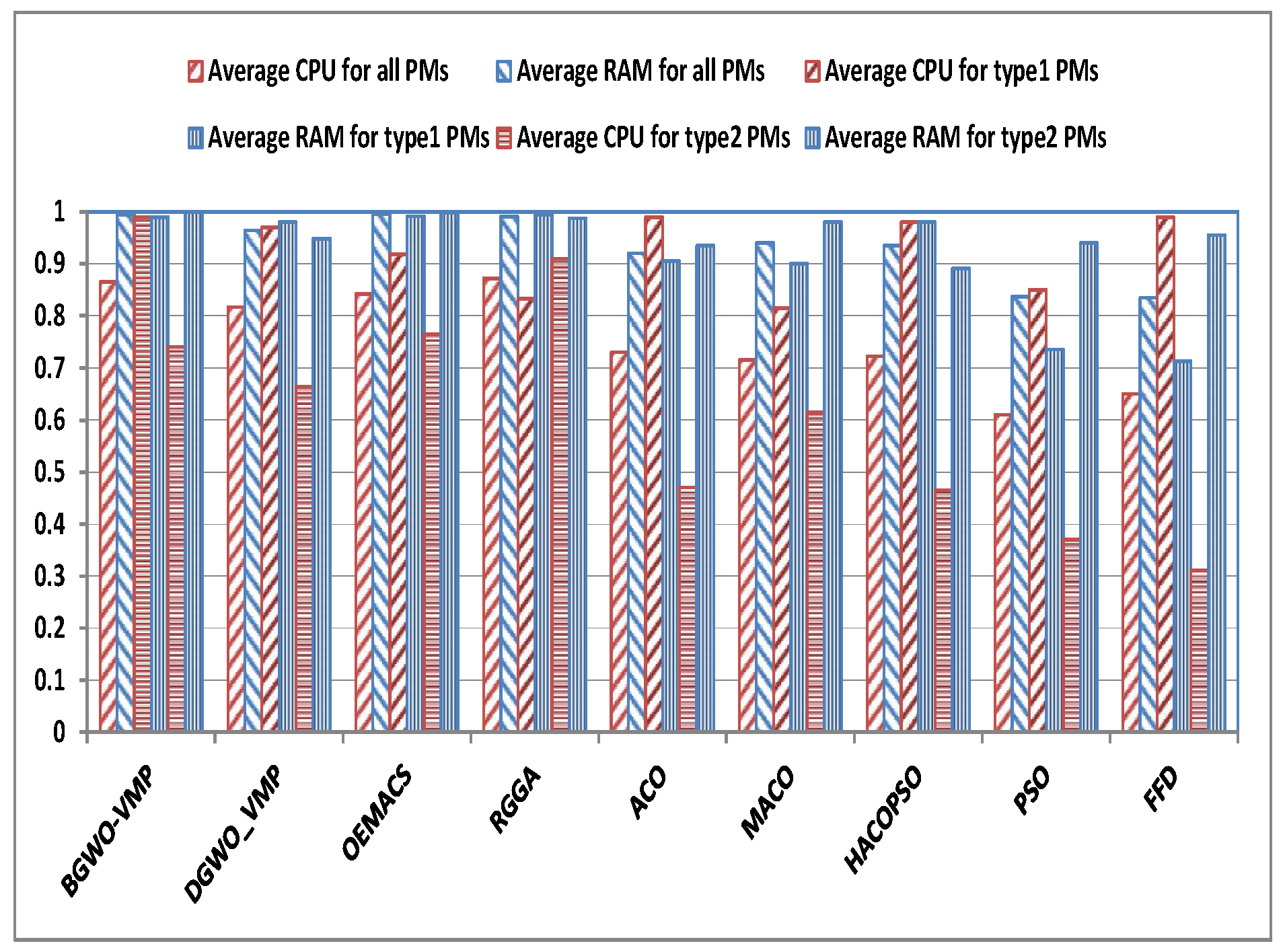
4.2. Large-Scale Heterogeneous Environmentt
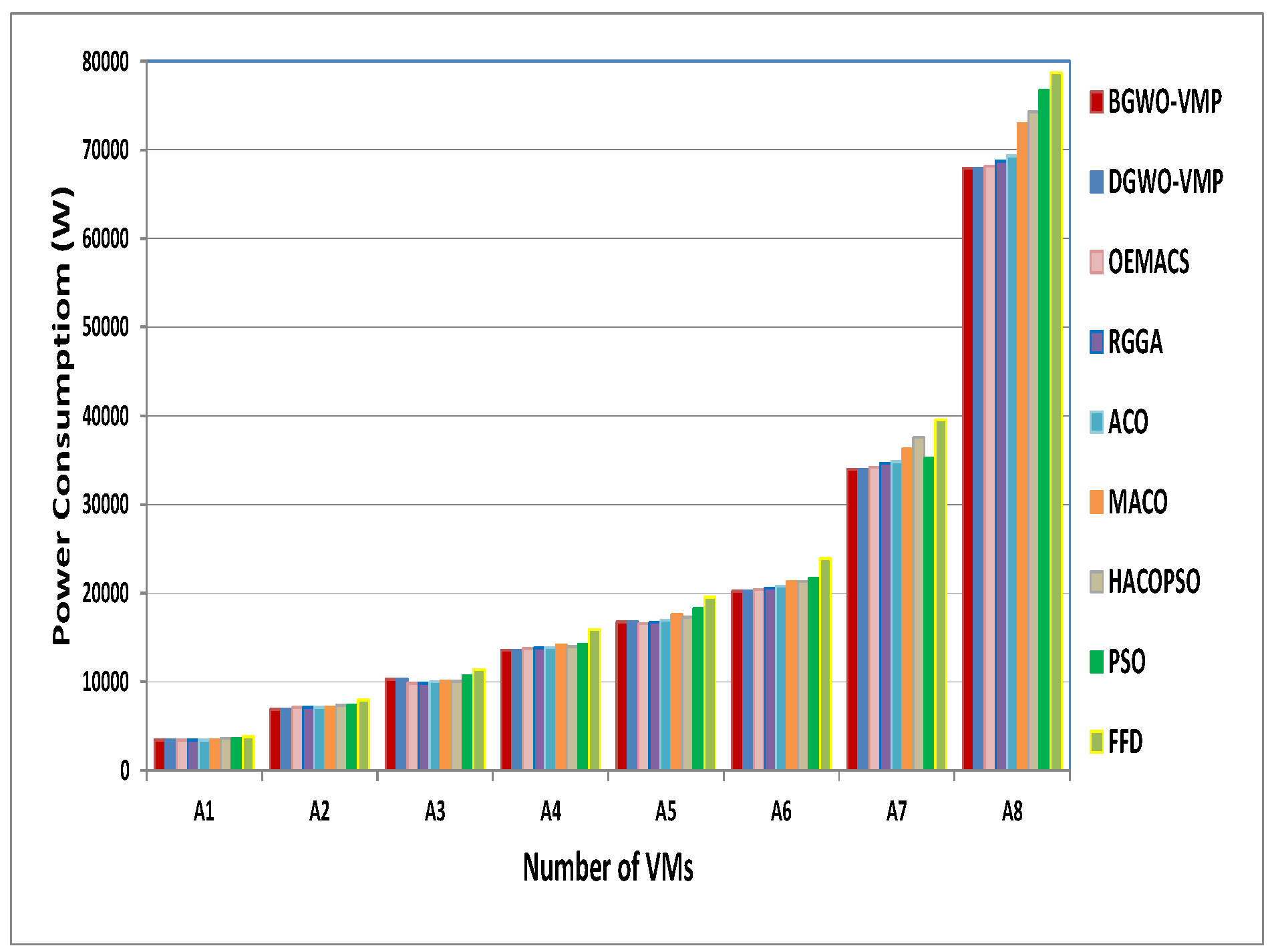
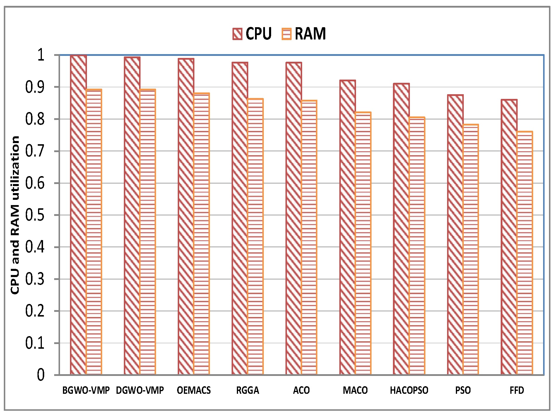
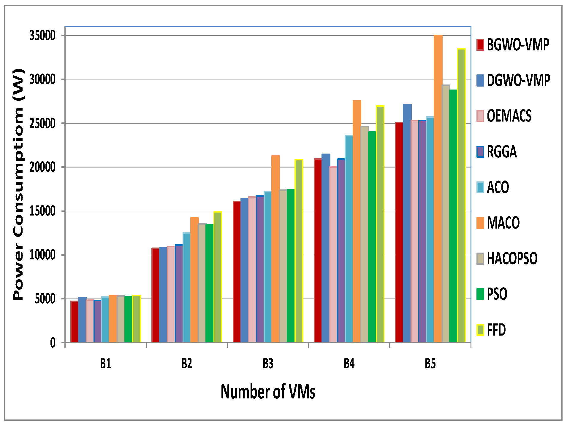
4.3. Power Consumption
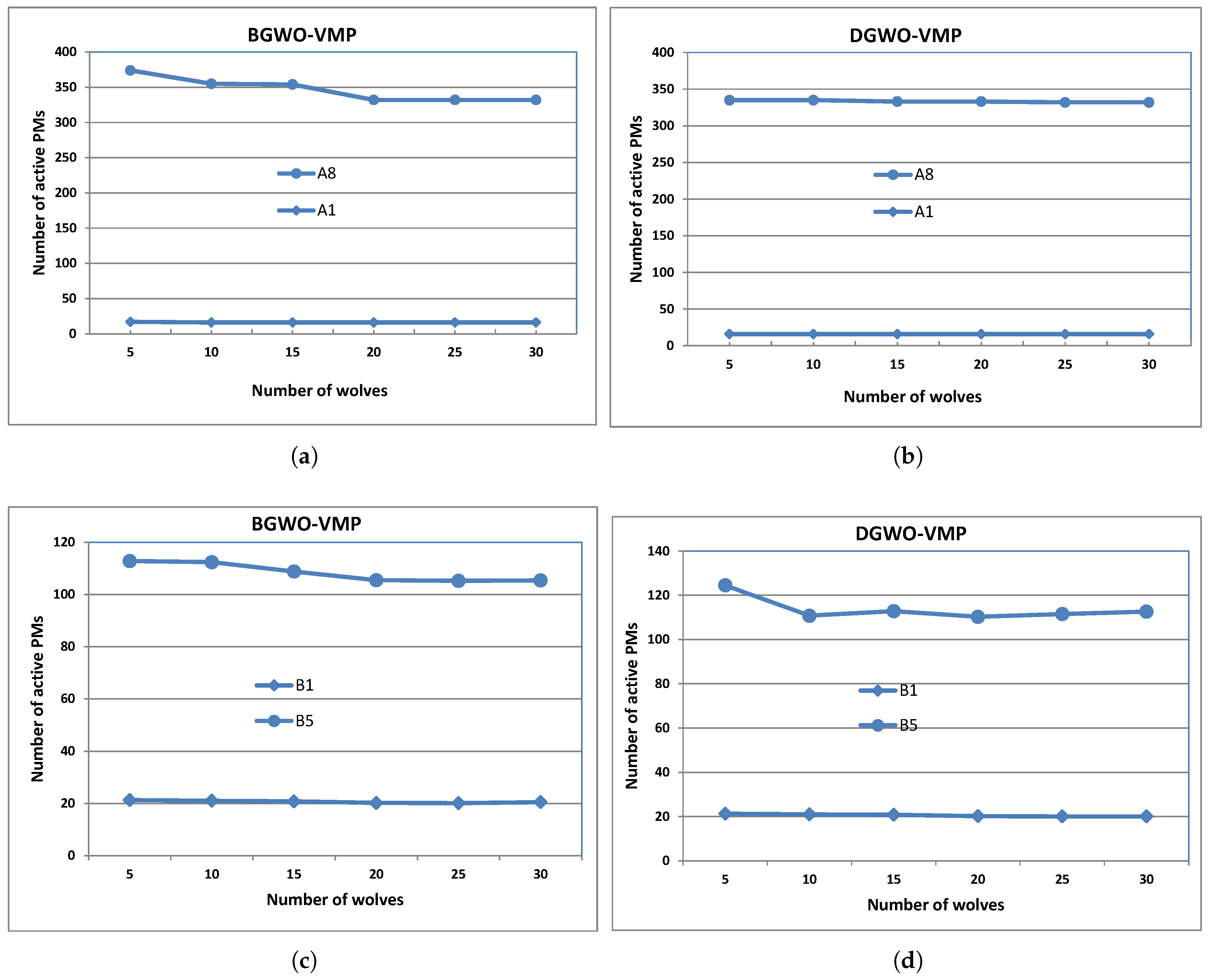
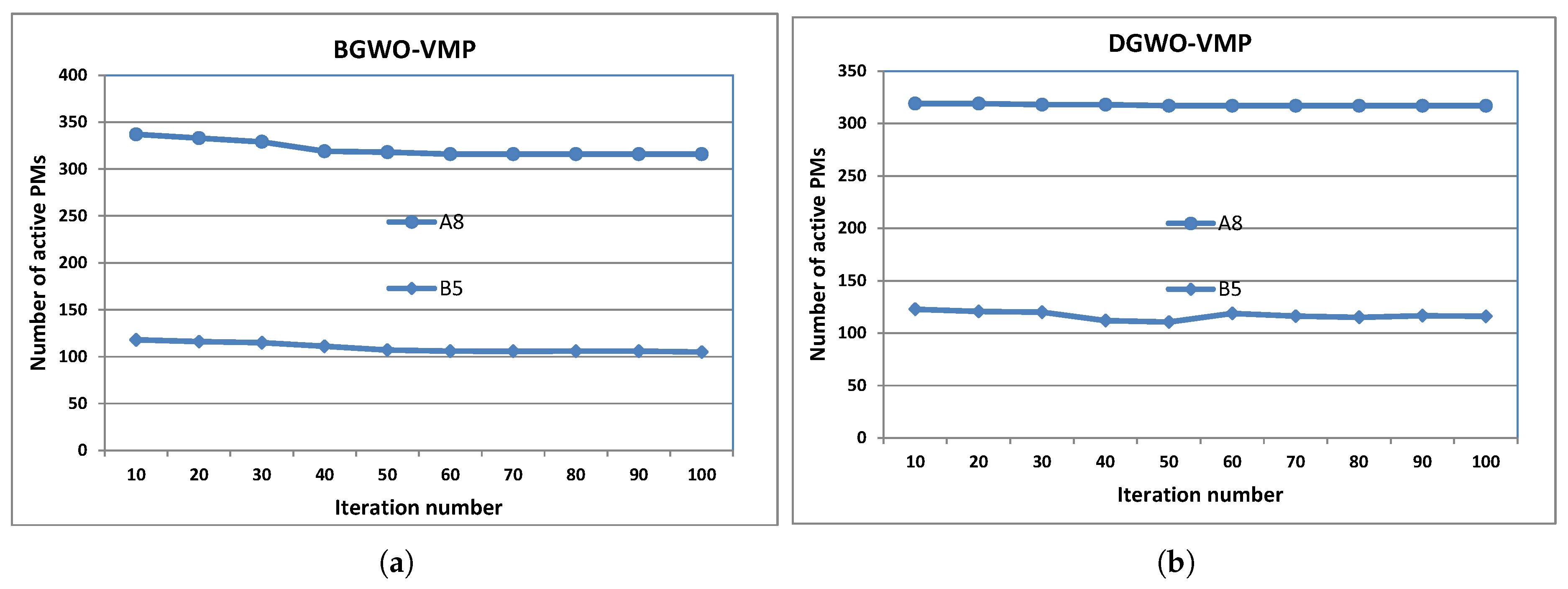
4.4. Further Analysis of BGWO-VMP and DGWO-VMP
5. Conclusions
Author Contributions
Funding
Conflicts of Interest
References
- Alford, T.; Morton, G. The Economics of Cloud Computing: Addressing the Benefits of Infrastructure in the Cloud; Booz Allen Hamilton: McLean, VG, USA, 2009. [Google Scholar]
- Zhang, Q.; Cheng, L.; Boutaba, R. Cloud computing: State-of-the-art and research challenges. J. Internet Serv. Appl. 2010, 1, 7–18. [Google Scholar] [CrossRef]
- Li, H.H.; Fu, Y.W.; Zhan, Z.H.; Li, J.J. Renumber strategy enhanced particle swarm optimization for cloud computing resource scheduling. In Proceedings of the 2015 IEEE Congress on. Evolutionary Computation (CEC), Sendai, Japan, 25–28 May 2015; pp. 870–876. [Google Scholar]
- Yang, B.; Li, Z.; Chen, S.; Wang, T.; Li, K. Stackelberg game approach for energy-aware resource allocation in data centers. IEEE Trans. Parallel Distrib. Syst. 2016, 27, 3646–3658. [Google Scholar] [CrossRef]
- Chen, Z.G.; Zhan, Z.H.; Li, H.H.; Du, K.J.; Zhong, J.H.; Foo, Y.W.; Li, Y.; Zhang, J. Deadline constrained cloud computing resources scheduling through an ant colony system approach. In Proceedings of the 2015 International Conference on Cloud Computing Research and Innovation (ICCCRI), Singapore, 26–27 October 2015; pp. 112–119. [Google Scholar]
- Mondal, S.K.; Muppala, J.K.; Machida, F. Virtual machine replication on achieving energy-efficiency in a cloud. Electronics 2016, 5, 37. [Google Scholar] [CrossRef]
- Mastroianni, C.; Meo, M.; Papuzzo, G. Probabilistic consolidation of virtual machines in self-organizing cloud data centers. IEEE Trans. Cloud Comput. 2013, 1, 215–228. [Google Scholar] [CrossRef]
- Yin, L.; Luo, J.; Luo, H. Tasks Scheduling and Resource Allocation in Fog Computing Based on Containers for Smart Manufacturing. IEEE Trans. Ind. Inform. 2018, 14, 4712–4721. [Google Scholar] [CrossRef]
- Mathew, V.; Sitaraman, R.K.; Shenoy, P. Energy-aware load balancing in content delivery networks. In Proceedings of the 2012 IEEE INFOCOM, Orlando, FL, USA, 25–30 March 2012; pp. 954–962. [Google Scholar]
- Mei, J.; Li, K.; Ouyang, A.; Li, K. A profit maximization scheme with guaranteed quality of service in cloud computing. IEEE Trans. Comput. 2015, 64, 3064–3078. [Google Scholar] [CrossRef]
- Hu, J.; Luo, J.; Li, K. Opportunistic Energy Cooperation Mechanism for Large Internet of Things. Mob. Netw. Appl. 2018, 23, 489–502. [Google Scholar] [CrossRef]
- Vogels, W. Beyond server consolidation. Queue 2008, 6, 20–26. [Google Scholar] [CrossRef]
- Tang, Z.; Ma, W.; Li, K.; Li, K. A data skew oriented reduce placement algorithm based on sampling. IEEE Trans. Cloud Comput. 2016. [Google Scholar] [CrossRef]
- Gupta, R.K.; Pateriya, R. Energy efficient virtual machine placement approach for balanced resource utilization in cloud environment. Int. J. Cloud-Comput. Super-Comput. 2015, 2, 9–20. [Google Scholar] [CrossRef]
- Cao, R.; Tang, Z.; Li, K.; Li, K. HMGOWM: A Hybrid Decision Mechanism for Automating Migration of Virtual Machines. IEEE Trans. Serv. Comput. 2018. [Google Scholar] [CrossRef]
- Chaisiri, S.; Lee, B.S.; Niyato, D. Optimal virtual machine placement across multiple cloud providers. In Proceedings of the 2009 IEEE Asia-Pacific Services Computing Conference (APSCC), Singapore, 7–11 December 2009; pp. 103–110. [Google Scholar]
- Speitkamp, B.; Bichler, M. A mathematical programming approach for server consolidation problems in virtualized data centers. IEEE Trans. Serv. Comput. 2010, 3, 266–278. [Google Scholar] [CrossRef]
- Wang, S.; Gu, H.; Wu, G. A new approach to multi-objective virtual machine placement in virtualized data center. In Proceedings of the 2013 IEEE Eighth International Conference on Networking, Architecture and Storage (NAS), Xi’an, China, 17–19 July 2013; pp. 331–335. [Google Scholar]
- Wilcox, D.; McNabb, A.; Seppi, K. Solving virtual machine packing with a reordering grouping genetic algorithm. In Proceedings of the 2011 IEEE Congress on Evolutionary Computation (CEC), New Orleans, LA, USA, 5–8 June 2011; pp. 362–369. [Google Scholar]
- Fatima, A.; Javaid, N.; Sultana, T.; Hussain, W.; Bilal, M.; Shabbir, S.; Asim, Y.; Akbar, M.; Ilahi, M. Virtual Machine Placement via Bin Packing in Cloud Data Centers. Electronics 2018, 7, 389. [Google Scholar] [CrossRef]
- Foo, Y.W.; Goh, C.; Lim, H.C.; Zhan, Z.H.; Li, Y. Evolutionary neural network based energy consumption forecast for cloud computing. In Proceedings of the 2015 International Conference on Cloud Computing Research and Innovation (ICCCRI), Singapore, 26–27 October 2015; pp. 53–64. [Google Scholar]
- Mirjalili, S.; Mirjalili, S.M.; Lewis, A. Grey wolf optimizer. Adv. Eng. Softw. 2014, 69, 46–61. [Google Scholar] [CrossRef]
- Emary, E.; Zawbaa, H.M.; Hassanien, A.E. Binary grey wolf optimization approaches for feature selection. Neurocomputing 2016, 172, 371–381. [Google Scholar] [CrossRef]
- Vaezi, M.; Zhang, Y. Virtualization and cloud computing. In Cloud Mobile Networks; Springer International Publishing: Basel, Switzerland, 2017; pp. 11–31. [Google Scholar]
- Tang, Z.; Mo, Y.; Li, K.; Li, K. Dynamic forecast scheduling algorithm for virtual machine placement in cloud computing environment. J. Supercomput. 2014, 70, 1279–1296. [Google Scholar] [CrossRef]
- Liu, X.F.; Zhan, Z.H.; Deng, J.D.; Li, Y.; Gu, T.; Zhang, J. An energy efficient ant colony system for virtual machine placement in cloud computing. IEEE Trans. Evolut. Comput. 2016, 22, 113–128. [Google Scholar] [CrossRef]
- Greenberg, A.; Hamilton, J.; Maltz, D.A.; Patel, P. The cost of a cloud: Research problems in data center networks. ACM SIGCOMM Comput. Commun. Rev. 2008, 39, 68–73. [Google Scholar] [CrossRef]
- Kusic, D.; Kephart, J.O.; Hanson, J.E.; Kandasamy, N.; Jiang, G. Power and performance management of virtualized computing environments via lookahead control. Clust. Comput. 2009, 12, 1–15. [Google Scholar] [CrossRef]
- Beloglazov, A.; Buyya, R.; Lee, Y.C.; Zomaya, A. A taxonomy and survey of energy-efficient data centers and cloud computing systems. In Advances in Computers; Elsevier: Amsterdam, The Netherlands, 2011; Volume 82, pp. 47–111. [Google Scholar]
- Barroso, L.A.; Hölzle, U. The case for energy-proportional computing. Computer 2007, 14, 33–37. [Google Scholar] [CrossRef]
- Fan, X.; Weber, W.D.; Barroso, L.A. Power provisioning for a warehouse-sized computer. In ACM SIGARCH Computer Architecture News; ACM: New York, NY, USA, 2007; Volume 35, pp. 13–23. [Google Scholar]
- Chen, M.; Zhang, H.; Su, Y.Y.; Wang, X.; Jiang, G.; Yoshihira, K. Effective VM sizing in virtualized data centers. In Proceedings of the 12th IFIP/IEEE International Symposium on Integrated Network Management. Citeseer, Dublin, Ireland, 23–27 May 2011; pp. 594–601. [Google Scholar]
- Lawey, A.Q.; El-Gorashi, T.E.; Elmirghani, J.M. Distributed energy efficient clouds over core networks. J. Lightw. Technol. 2014, 32, 1261–1281. [Google Scholar] [CrossRef]
- Eusuff, M.; Lansey, K.; Pasha, F. Shuffled frog-leaping algorithm: A memetic meta-heuristic for discrete optimization. Eng. Optim. 2006, 38, 129–154. [Google Scholar] [CrossRef]
- Kansal, N.J.; Chana, I. Artificial bee colony based energy-aware resource utilization technique for cloud computing. Concurr. Comput. Pract. Exp. 2015, 27, 1207–1225. [Google Scholar] [CrossRef]
- Wu, Y.; Tang, M.; Fraser, W. A simulated annealing algorithm for energy efficient virtual machine placement. In Proceedings of the 2012 IEEE International Conference on Systems, Man, and Cybernetics (SMC), Seoul, Korea, 14–17 October 2012; pp. 1245–1250. [Google Scholar]
- Cho, K.M.; Tsai, P.W.; Tsai, C.W.; Yang, C.S. A hybrid meta-heuristic algorithm for VM scheduling with load balancing in cloud computing. Neural Comput. Appl. 2015, 26, 1297–1309. [Google Scholar] [CrossRef]
- Wen, W.T.; Wang, C.D.; Wu, D.S.; Xie, Y.Y. An aco-based scheduling strategy on load balancing in cloud computing environment. In Proceedings of the 2015 Ninth International Conference on Frontier of Computer Science and Technology (FCST), Dalian, China, 26–28 August 2015; pp. 364–369. [Google Scholar]
- Feller, E.; Rilling, L.; Morin, C. Energy-aware ant colony based workload placement in clouds. In Proceedings of the 2011 IEEE/ACM 12th International Conference on Grid Computing, Lyon, France, 21–23 September 2011; IEEE Computer Society: Washington, DC, USA, 2011; pp. 26–33. [Google Scholar]
- Tawfeek, M.A.; El-Sisi, A.B.; Keshk, A.E.; Torkey, F.A. Virtual machine placement based on ant colony optimization for minimizing resource wastage. In International Conference on Advanced Machine Learning Technologies and Applications; Springer: Cham, Switzerland, 2014; pp. 153–164. [Google Scholar]
- Suseela, B.B.J.; Jeyakrishnan, V. A multi-objective hybrid ACO–PSO optimization algorithm for virtual machine placement in cloud computing. Int. J. Res. Eng. Technol. 2014, 3, 474–476. [Google Scholar]
- Abdessamia, F.; Tai, Y.; Zhang, W.Z.; Shafiq, M. An Improved Particle Swarm Optimization for Energy-Efficiency Virtual Machine Placement. In Proceedings of the 2017 International Conference on Cloud Computing Research and Innovation (ICCCRI), Singapore, 11–13 April 2017; pp. 7–13. [Google Scholar]
- Braiki, K.; Youssef, H. Multi-Objective Virtual Machine Placement Algorithm Based on Particle Swarm Optimization. In Proceedings of the 2018 14th InternationalWireless Communications & Mobile Computing Conference (IWCMC), Singapore, 11–12 April 2018; pp. 279–284. [Google Scholar]
- Buyya, R.; Ranjan, R.; Calheiros, R.N. Modeling and simulation of scalable Cloud computing environments and the CloudSim toolkit: Challenges and opportunities. In Proceedings of the 2009 International Conference on High Performance Computing & Simulation, Leipzig, Germany, 21–24 June 2009; pp. 1–11. [Google Scholar]
- Ajiro, Y.; Tanaka, A. Improving packing algorithms for server consolidation. In Proceedings of the International CMG Conference, San Diego, CA, USA, 2–7 December 2007; Volume 253, pp. 399–406. [Google Scholar]
- Cavdar, M.C. A Utilization Based Genetic Algorithm for Virtual Machine Placement in Cloud Computing Systems. Ph.D. Thesis, Bilkent University, Ankara, Turkey, 2016. [Google Scholar]


| No. | M | BGWO | DGWO | OEMACS | RGGA | ACO | MACO | HACOPSO | PSO | FFD |
|---|---|---|---|---|---|---|---|---|---|---|
| A1 | 100 | 16 | 16 | 16 | 16 | 16 | 16 | 16.93 | 17 | 18 |
| A2 | 200 | 32 | 32 | 33 | 33 | 33 | 33 | 34 | 34 | 37 |
| A3 | 300 | 48 | 48 | 46 | 46.03 | 46.63 | 47 | 47 | 50 | 53 |
| A4 | 400 | 63 | 63 | 64 | 64.3 | 64.33 | 65.9 | 65.1 | 66 | 74 |
| A5 | 500 | 78 | 78 | 77 | 77.63 | 78.93 | 81.93 | 80.5 | 85 | 91 |
| A6 | 600 | 94 | 94 | 95 | 95.77 | 96.73 | 99.16 | 99.2 | 101 | 111 |
| A7 | 1000 | 158 | 158 | 159 | 161.23 | 161.86 | 168.86 | 174.66 | 164 | 184 |
| A8 | 2000 | 316 | 316 | 317 | 319.64 | 322.73 | 339.33 | 345.66 | 357 | 366 |
| No. | M | BGWO | DGWO | OEMACS | RGGA | ACO | MACO | HACOPSO | PSO | FFD |
|---|---|---|---|---|---|---|---|---|---|---|
| B1 | 100 | 19 | 20.2 | 19 | 19.33 | 23.13 | 28.267 | 24.56 | 21 | 32 |
| B2 | 200 | 43.2 | 44 | 45 | 45.26 | 55.26 | 68.26 | 57.76 | 57.2 | 75 |
| B3 | 300 | 64 | 66 | 68 | 68 | 79.13 | 106.86 | 79.36 | 79.4 | 102 |
| B4 | 400 | 85.5 | 89 | 81 | 82.36 | 103.06 | 137.16 | 114.4 | 105 | 131 |
| B5 | 500 | 105.7 | 110.3 | 107 | 107.96 | 127.06 | 178.36 | 133.66 | 130 | 167 |
© 2019 by the authors. Licensee MDPI, Basel, Switzerland. This article is an open access article distributed under the terms and conditions of the Creative Commons Attribution (CC BY) license (http://creativecommons.org/licenses/by/4.0/).
Share and Cite
Al-Moalmi, A.; Luo, J.; Salah, A.; Li, K. Optimal Virtual Machine Placement Based on Grey Wolf Optimization. Electronics 2019, 8, 283. https://doi.org/10.3390/electronics8030283
Al-Moalmi A, Luo J, Salah A, Li K. Optimal Virtual Machine Placement Based on Grey Wolf Optimization. Electronics. 2019; 8(3):283. https://doi.org/10.3390/electronics8030283
Chicago/Turabian StyleAl-Moalmi, Ammar, Juan Luo, Ahmad Salah, and Kenli Li. 2019. "Optimal Virtual Machine Placement Based on Grey Wolf Optimization" Electronics 8, no. 3: 283. https://doi.org/10.3390/electronics8030283
APA StyleAl-Moalmi, A., Luo, J., Salah, A., & Li, K. (2019). Optimal Virtual Machine Placement Based on Grey Wolf Optimization. Electronics, 8(3), 283. https://doi.org/10.3390/electronics8030283