Abstract
In this paper, we propose a new dimensionality reduction method named Discriminative Sparsity Graph Embedding (DSGE) which considers the local structure information and the global distribution information simultaneously. Firstly, we adopt the intra-class compactness constraint to automatically construct the intrinsic adjacent graph, which enhances the reconstruction relationship between the given sample and the non-neighbor samples with the same class. Meanwhile, the inter-class compactness constraint is exploited to construct the penalty adjacent graph, which reduces the reconstruction influence between the given sample and the pseudo-neighbor samples with the different classes. Then, the global distribution constraints are introduced to the projection objective function for seeking the optimal subspace which compacts intra-classes samples and alienates inter-classes samples at the same time. Extensive experiments are carried out on AR, Extended Yale B, LFW and PubFig databases which are four representative face datasets, and the corresponding experimental results illustrate the effectiveness of our proposed method.
1. Introduction
In recent years, face recognition has attracted many researches for various applications in the field of artificial intelligence, such as identity authentication, age progression and human-computer interaction [1,2,3]. However, since the unconstrained face images captured in the real scene are influenced by illumination, posture, expression, occlusion, age and other unpredictable interference factors, the performance of face recognition is limited. At present, Sparse Representation (SR) [4,5] and Deep Learning (DL) [6,7] technologies have been effectively applied to unconstrained face recognition and achieved impressive results.
Considering the complexity of the DL-based algorithms, appearance-based subspace learning algorithms have attracted considerable interest due to their simplicity and desirable performance. Since unconstrained face images present a distorted nonlinear distribution in the high-dimensional sample space [8,9], dimensionality reduction is usually exploited to extract the accurate low-dimensional intrinsic structure embedded in the high-dimensional sample space, which not only reduces classification time but also increases the prediction accuracy and strengthens the generalization ability. Thus, dimensionality reduction is crucial for unconstrained face recognition and received tremendous attentions in past 20 years.
The classical dimensionality reduction methods represented by Principal Component Analysis (PCA) [10] and Linear Discriminant Analysis (LDA) [11] have been widely utilized in various fields for the advantages of concise mathematical theory and low computational cost [12,13,14]. However, these types of methods only consider the global linear distribution of data and ignore the characteristics of local intrinsic structures. In recent years, it has been found that face images lie on a low-dimensional manifold structure embedded in the high-dimensional sample space. Inspired by this, researchers proposed many nonlinear dimensionality reduction methods based on manifold learning [15,16,17], such as Local Linear Embedding (LLE) [18], Laplacian Eigenmaps (LE) [19], ISOMAP [20], etc. In view of Out-Of-Sample extension problem [21] in manifold learning, He et al. proposed Locality Preserving Projections (LPP) [22] and Neighborhood Preserving Embedding (NPE) [23] to improve LE and LLE, respectively, which tackle the nonlinear mapping process with a linear approximation. Subsequently, numerous LPP-based and NPE-based methods were widely presented and used in the field of pattern recognition [24,25,26,27].
Yan et al. [28] indicated that these subspace learning methods can be unified in the Graph Embedding Framework (GEF). The key idea is to seek an optimal low-dimensional subspace according to the adjacent graph predefined in the high-dimensional sample space. The traditional construction of adjacent graph usually adopts k-nearest [29] or ε-ball [23] to select nearby points of adjacent graph, and employs heat kernel function [29] or inverse Euclidean distance [30] to assign weights between nearby points. However, the distribution of real data is complex and unknown in most cases. It is very difficult to select the appropriate parameters for adjacent graph in GEF.
As a type of signal representation method, Sparse Representation (SR) [31,32] searches for the most compact representation of a given sample concerning the linear combination of a series of training samples. The obtained representation coefficients can reflect the similarity between samples, namely the bigger the coefficients are, the more likely these samples belong to the same class. By exploiting this characteristic of sparse representation in adjacent graph construction, Qiao et al. [33] proposed the Sparsity Preserving Projections (SPP) algorithm, in which the selected training samples for linear combination are the nearby points of adjacent graph, and the representation coefficients are the reconstruction weights between the given sample and the selected training samples. Thus, it is clear that SPP can automatically construct the adjacent graph by sparse representation, and effectively overcomes the shortcoming of predefining adjacent graph in the traditional graph embedding framework. This new idea of adjacent graph construction has received widespread attention of scholars at home and abroad [34,35]. Subsequently, a large number of excellent algorithms have emerged. Lai et al. [36] introduced sparse representation into LLE and proposed Sparse Linear Embedding (SLE) algorithm and its kernel extension. Extensive experiments on three face databases and two object databases demonstrated the effectiveness of the methods, especially in the case of small samples. Yin et al. [37] proposed Local Sparsity Preserving projection (LSPP) and achieved good results on biological databases. Zhang et al. [38] presented Sparsity and Neighborhood Preserving Projections (SNPP) algorithm by utilizing the advantages of SPP and NPE for face recognition.
Although SPP has been widely utilized, its performance is affected by the unsupervised characteristic. In unconstrained face recognition, face images collected in the real scene are influenced by illumination, posture, expression, occlusion, age and other unpredictable interference factors. These factors introduce great diversity to samples which causes the difference between intra-class samples and the similarity between inter-class samples. Therefore, the reconstruction weights of SPP can not imply label information of samples which restricts the discriminating capability. To address this problem, Lu et al. [39] proposed Discriminant Sparsity Neighborhood Preserving Embedding (DSNPE) algorithm, which introduced the label information into sparse graph construction. It is a supervised dimensionality reduction method in which the given sample is not only reconstructed by a series of samples with the same class, but also is represented as a linear combination of samples with different classes. Wei et al. [40] presented Weighted Discriminative Sparsity Preserving Embedding (WDSPE) algorithm by introducing reconstruction weights constraint of samples on the basis of DSNPE. Lou et al. [41] proposed Graph Regularized Sparsity Discriminant Analysis (GRSDA) algorithm by combining SR with LPP. Huang et al. [42] provided Regularized Coplanar Discriminant Analysis (RCDA) algorithm in which the samples from the same class are coplanar and the samples from different classes are not coplanar.
These above supervised learning methods [39,40,41,42] utilize the local neighborhood information of intra-class samples and inter-class samples respectively, but they ignore the global distribution information of all samples in space. In fact, researchers have shown that the global geometric structure of data sets implies useful discriminative information which is important for image identification [43,44]. In this paper we propose a new dimensionality reduction named Discriminative Sparsity Graph Embedding (DSGE) which considers the local structure information and global distribution information simultaneously. To be specific, we make improvements on two aspects for further boosting discriminating capability and generalization ability. (1) In the procedure of adjacent graph construction, we firstly introduce the intra-class compactness constraint into the construction of intrinsic adjacent graph for enhancing the neighborhood reconstruction relationship of samples with the same class. Meanwhile the inter-class compactness constraint is also exploited in penalty adjacent graph construction for further weakening the neighborhood reconstruction influence of samples with the different classes. (2) In the process of low-dimensional projections, we respectively add the global intra-class distribution constraint and global inter-class distribution constraint into the intra-class scatter and inter-class scatter, and seek the optimal subspace by taking advantage of maximum margin criterion (MMC) [45] such that samples from the same class are more compact, while samples from different classes are more distant.
The organization of the rest of this paper is as follows: Section 2 presents an overview of the related works. In Section 3 we describe the detailed steps of Discriminative Sparsity Graph Embedding. In Section 4 we provide the experimental results and performance analysis. Section 5 gives the conclusion.
2. Related works
2.1. Sparse Representation
Sparse representation is a type of signal representation method spreading after wavelet transform and multi-scale geometric analysis [31,32]. The basic idea is to approximately represent the given sample by a linear combination of a few (sparse) atoms in an over-complete dictionary. The objective function is as follows:
where is the given sample vector, is the over-complete dictionary matrix, and is the obtained representation coefficient vector. In Equation (1), is the -norm which denotes the number of non-zero entries in the vector . However, owing to the NP problem of -norm optimization, it is substituted with -norm and the objective function is modified as:
After obtaining the optimal representation coefficient vector , the label of is finally determined as the class with the minimal reconstructive error as described in [31].
where is the sparse coefficients of the given sample represented by the ith class training samples ().
2.2. Sparsity Preserving Projections
Motivated by sparse representation, Qiao et al. [33] proposed Sparsity Preserving Projections (SPP) algorithm. The objective function is as follows:
where is the projection matrix and is the whole training set including samples. Furthermore is an arbitrary sample and is the corresponding reconstruction weights which can be solved by Equation (5):
in which is different from which is composed of all training samples except for , and is a vector of all ones. We utilize the constraint term to normalize the sparse reconstruction weights of .
SPP adopts sparse representation as a way to automatically construct adjacent graphs which overcomes the limitation of artificially constructing adjacent graphs in the traditional manifold learning. It seeks the optimal low-dimensional subspace by maintaining the reconstruction relationship between and obtained in the high-dimensional sample space. However, due to the complexity of unconstrained face images, the neighborhood reconstruction relationship residing in adjacent graph via SPP algorithm is not accurate. Figure 1 gives an example on the LFW database [46]. We randomly select one sample as and the remaining 99 samples as . The corresponding reconstruction weight of is calculated by Equation (5). As shown in the Figure 1, there are 100 samples participating in the reconstruction of , where the first 10 samples possess the same class label as and the remaining 90 samples have different ones. It can be seen that the reconstruction weights of some samples with different labels as are fairly large, such as the 29th, 39th, 48th and 65th samples, while the reconstruction weights of other samples with the same label as are zeros except for 4th and 8th. It means that the adjacent graph of SPP neglects some intra-class samples which are non-neighbor due to the interference of unpredictable factors in the same subject, and has the potential to connect a few inter-class samples which are pseudo-neighbor in view of similar face compositions in different subjects.
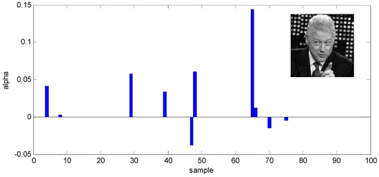
Figure 1.
Sparsity reconstruction weights of one sample by Sparsity Preserving Projections (SPP) algorithm on the LFW database.
3. Discriminative Sparsity Graph Embedding
As described in the aforementioned analysis, SPP ignores the label information of samples and cannot well exhibit the local neighborhood relationship of adjacent graph. Although a few improved algorithms [39,40,41,42] have been proposed, their performance is still limited. In this paper, we propose a DSGE which consists of two improvements on adjacent graph construction and low dimensional projection, respectively. In the following section, we explain the implementation process of the above two improvements in detail.
3.1. Adjacent Graph Construction
Let be the whole training set and denote the ith subset including training samples. We first construct the intrinsic adjacent graph with the intra-class weight matrix by the following objective function:
where is the jth sample selected in the ith subset and denotes the class label of . is composed of all samples from except for , and the obtained is the corresponding intra-class reconstruction weight of . To avoid the omission of non-neighbor samples from the same class in the intrinsic adjacent graph, we additionally add the intra-class compactness constraint in Equation (6) which is represented as the average value of intra-class reconstruction weights of all samples belonging to . It can further enhance the reconstruction relationship between and the remaining samples in the subset .
Zhang et al. [47] have demonstrated that -norm regularization can obtain similar results as -norm regularization but is much less time consuming. Hence in the procedure of sparse regularization, we substitute -norm with -norm as shown in Equation (6). Meanwhile, since and are highly interrelated, we adopt a rapid optimization algorithm of Equation (6) rather than traditional alternating algorithm [48], which is exhibited in detail as follows:
| Algorithm 1 The intra-class reconstruction weight optimization algorithm (Solving Equation (6)) |
| Input: Any sample and its intra-class reconstruction dictionary . Set the initial intra-class compactness constraint and the initial intra-class reconstruction weight as zero vectors. Iteration . Output: The optimum intra-class reconstruction weight |
| Step 1: Successively calculate the intra-class reconstruction weights of all samples belonging to the ith subset by the following function which is derived from Equation (6) (). Step 2: Calculate the intra-class compactness constraint . Step 3: If or , output , otherwise set and return to Step 1. |
After getting the intra-class reconstruction weights of all samples from the ith subset , we assign them into the sub-matrix denoted herein as , and the intra-class weight matrix of the whole training set is represented as:
Similar to the construction process of intrinsic adjacent graph, we also get the penalty adjacent graph with the inter-class weight matrix . The objective function of inter-class reconstruction weight of is calculated by:
where which excludes . For further weakening the reconstruction relationship between and other samples with the different classes, we also adopt the inter-class compactness constraint in Equation (9) which is equal to the average value of inter-class reconstruction weights of all samples in the subset . The optimal inter-class reconstruction weights are computed via the similar procedure as that of Equation (6).
| Algorithm 2 The inter-class reconstruction weight optimization algorithm (Solving Equation (9)) |
| Input: Any sample and its inter-class reconstruction dictionary . Set the initial inter-class compactness constraint and the initial inter-class reconstruction weight as zero vectors. Iteration . Output: The optimum inter-class reconstruction weight . |
| Step 1: Successively calculate the inter-class reconstruction weights of all samples belonging to the ith subset by the following function which is derived from Equation (9). () Step 2: Calculate the intra-class compactness constraint . Step 3: If or , output , otherwise set and return to Step 1. |
In view of expediently representing the inter-class weight matrix, we extend to N-dimensional vector denoted as , and the inter-class reconstruction weight sub-matrix of is expressed as:
So the inter-class weight matrix of the whole training set is straightforward represented as:
3.2. Objective Function of DSGE
As the previous discussion, while maintaining the local structure of intra-class and inter-class samples, DSGE introduces the global intra-class distribution constraint to intra-class scatter and the global inter-class distribution constraint to inter-class scatter to compact the same class samples and alienate the different class samples, respectively. Here, we design the cost functions as follows:
where describes the reconstruction relationship between and which belongs to the same class. represents the reconstruction relationship between and which belongs to the different classes. In Equation (13) the global intra-class distribution constraint is defined as where is the average matrix of . Similarly in Equation (14), the global inter-class distribution constraint is represented by where is the average matrix of all training samples. Equation (13) can be formulated as:
where . Similarly, Equation (14) can be computed as:
where .
Motivated by the idea of MMC, we maximize intra-class scatter and minimize inter-class scatter at the same time. The final objective function of DSGE as follows:
Substituting Equations (15) and (16) into Equation (17), we can get
By using the Lagrangian multiplier method, in the condition of , the optimal projection matrix is calculated by the following eigen equation:
We select the corresponding eigenvectors of the top eigenvalues and get the optimal projection matrix .
Figure 2 illustrates the results of two-dimensional projection by SPP [33], DSNPE [39], and the proposed DSGE respectively on the Extended Yale B database. As can be seen, the corresponding projection subsets of four different individuals randomly selected from the database are the least distant based on SPP algorithm. Furthermore, there are some intersections across subsets as shown in Figure 2a. In Figure 2b, the layout of samples of DSNPE is better than that of SPP, but the distribution of samples in each subset is still not compact enough. As depicted in Figure 2c, the proposed DSGE algorithm makes the samples of the same class as compact as possible, and keep the samples of different classes as distant as possible. So it can be seen that DSGE has the optimum projection performance which facilitates the succeeding classification task.
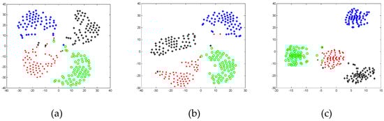
Figure 2.
Results of two-dimensional projection on the Extended Yale B. (a) SPP; (b) DSNPE; (c) DSGE (the points of different colors represent the different subjects).
3.3. Unconstrained Face Recognition Based on DSGE
In this paper, our proposed DSGE algorithm is applied to unconstrained face recognition for dimensionality reduction. The specific steps are as follows:
Step 1. Calculate the intra-class reconstruction weight and the inter-class reconstruction weight of each sample by Equations (6) and (9) respectively;
Step 2. Compute the intra-class weight matrix and the inter-class weight matrix by Equations (8) and (12), respectively;
Step 3. Select the corresponding eigenvectors of the top eigenvalues, which is calculated by Equation (19), and construct the optimal low-dimensional projection matrix ;
Step 4. Map training samples and test samples to the corresponding low-dimensional manifold subspaces respectively by the following formulas:
Step 5. Adopt the low dimensional subspace of training samples to train classifier, and employ test sample to verify the identification performance.
4. Experiments and Analysis
To fully verify the effectiveness of the proposed DSGE algorithm, we conducted extensive experiments on two categories of face databases. One includes the AR database [49] and the Extended Yale B database [50] which are captured in strictly controlled environments, the other contains the LFW database [46] and the PubFig database [51] which are collected in real environments. PCA [10] was applied as a preprocessing step for avoiding matrix singularity, and 98% of the image energy is retained.
4.1. Experiments on the AR Database
The AR database contains over 4000 frontal-view face images of 126 individuals with different facial expressions, lighting conditions, and occlusions (including sunglasses and scarves). These images were collected under strictly controlled experimental conditions. In this section, we selected 3120 images of 120 individuals (65 males and 55 females) which were taken in two sessions (separated by two weeks), and each session of one individual contains 13 face images in which the first four images are interfered by expression, the fifth to seventh images are influenced by light conditions, and the remaining six images have occlusion interference factors (three images with sunglass and three images with scarf). Figure 3 provides some samples of one individual in two sessions and the face portion of each image was normalized to 50 × 40 pixels. In this section, we do three experiments for proving the effectiveness of DSGE on the AR database.
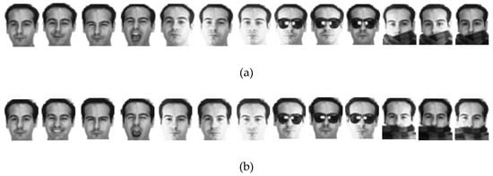
Figure 3.
Samples of one individual in two sessions on the AR database. (a) Samples in the first session; (b) samples in the second session.
Experiment 1: We first evaluated the effectiveness of DSGE against the interference of expression change and light condition of facial images on the AR database. In this experiment, we selected seven images without occlusions in session one for training, and choose the corresponding seven images in session two for testing. Since the training samples and testing samples were selected from two different sessions, the influence of time variation residing in facial images still needs to be considered. We respectively used LDA [11], LPP [22], NPE [23], SPP [33], DSNPE [39], DP-NFL [52], SRC-DP [53] and the proposed DSGE for dimensionality reduction respectively, and exploited SRC classifier for face recognition, in which L1-Ls [54] was adopted to calculate the sparse representation coefficients. The recognition rate of each method and the corresponding dimension are listed in Table 1. In detail DSGE achieved the best performance with 12.74%, 10.24%, 8.69%, 9.17%, 1.31%, 5.58% and 2.18% improvements over LDA, LPP, NPE, SPP, DSNPE, DP-NFL and SRC-DP, respectively. Thus it can be seen that DSGE was not only unaffected by the interference of facial expression and light condition, but also effectively overcame the influence of time variation on human face.

Table 1.
The recognition rate and the corresponding dimension of each method on the AR databases.
Meanwhile, we randomly selected the total seven images without occlusions in session one and session two for training, and the remaining seven images for testing. Figure 4 gives the maximal recognition rate versus the variation of dimension. From it, we can see that DSGE outperformed other methods when the dimension is larger than 30. Therefore DSGE is insensitive to variations of dimension and can well characterize the discriminative structure of facial images disturbed by facial expression, light condition and time variation.
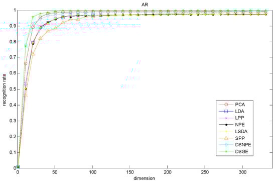
Figure 4.
Recognition rate vs. variation of dimension on the AR database.
Experiment 2: We further demonstrated the effectiveness of DSGE against the interference of real occlusion on the AR database. In this experiment, we assessed it from three aspects. (1) Sunglass occlusion. We selected seven images without occlusion and one image with sunglass in session one for training, and choose seven images without occlusion in session two and the remaining five images with sunglass in session one and session two for testing. (2) Scarf occlusion. The selection of samples is similar to the above. We selected seven images without occlusion and one image with scarf in session one for training, and choose seven images without occlusion in session two and the remaining five images with scarf in session one and session two for testing. (3) Mixed occlusion of sunglass and scarf. We selected seven images without occlusion and one image with sunglass and one image with scarf in session one for training, and choose the remaining images in session one and the whole images in session two for testing. Table 2 presents the recognition rate of these methods under three real occlusion conditions. Although the performance of DSGE is slightly lower than that of SRC-DP under sunglass occlusion and scarf occlusion, it outperforms all the other methods by more than 2% under the mixed occlusion. Therefore it can be seen that DSGE is more conducive to obtaining the intrinsic manifold structure embedded in the mixed occlusion images.
Table 2.
The recognition rate of each method under three kinds of real occlusion on the AR databases.
Experiment 3: We comprehensively assessed the performance of DSGE against all the interference including facial expression, light condition, real occlusion and time variation on the AR database. In this experiment we randomly selected the total 13 images in session one and session two for training, and choose the remaining 13 images for testing. We repeated this process 10 times by using 1NN classifier and SVM classifier respectively, and then obtained the experimental results as shown in Table 3. From it, we can see that DSGE was still superior to other methods which means that the proposed DSGE was free from the influence of mixed interference factors, and can well characterize the underlying manifold structure of data.
Table 3.
Experimental results with the mixed interference factors on the AR database.
4.2. Experiments on the Extended Yale B Database
The Extended Yale B database contains 2414 frontal-face images of 38 individuals with different light conditions. Each individual had about 64 images. These images were resized to 32 × 32 pixels, and some samples of one person are shown in Figure 5. In this section, we did two experiments for evaluating the performance of DSGE on the Extended Yale B database.

Figure 5.
Some samples of one person with different light conditions on the Extended Yale database.
Experiment 1: First, for proving the effectiveness of DSGE against the interference of illumination with different degrees on the Extended Yale B database, we randomly selected N images of each individual as training samples, and the remaining 64–N images were used as test samples. In this experiment, the value of N is 10, 20 or 30. In order to facilitate the comparison with the state-of-the-art algorithm named GRSDA [41], we adopted the nearest neighbor classifier with the identical settings as GRSDA to conduct experiments. The best recognition rate of each method and the corresponding dimension are listed in Table 4. It should be noted that the experimental results of methods except for DSGE in Table 4 are all cited from Ref [41]. From it, we observed that whether the number of training samples is 10, 20 or 30, DSGE was always superior to the other methods and it outperformed GRSDA by 6.58%, 6.25% and 4.79% respectively. This demonstrates that the proposed DSGE has the ability of eliminating the interference of light change and is insensitive to the number of training samples.
Table 4.
The best recognition rate and the corresponding dimension of each method on the Extended Yale B databases.
Experiment 2: For further demonstrating the effectiveness of DSGE against occlusion on the Extended Yale B database, we randomly selected 14 images of each individual and added noise occlusion block with black and white dots with random distribution. The location of noise occlusion block was random and the ratio of size between noise occlusion block and original image was also random where the ratio parameter ranged from 0.05 to 0.15. Some occlusion samples of one person are depicted in Figure 6. In this section, we did the following experiments by two cases. (1) We randomly selected 32 images per person which included 14 images with noise occlusion block, and the remaining images for testing. (2) We randomly selected 32 images per person which contained seven images with noise occlusion block, and the remaining images for testing. All experiments in each case were conducted by 1NN classifier and SVM classifier respectively, and were repeated 10 times. The experimental results are shown in Table 5. From it, we observed that despite the location and size of noise occlusion block in facial images being random, the performance of DSGE was still not affected. By using the 1NN classifier and SVM classifier in the first case, the average accuracy and standard deviation of DSGE were 94.84 ± 1.82% and 95.96 ± 0.87%, respectively, which ranked the highest. When reducing the number of occlusion images, such as in case two, the recognition accuracy of DSGE also increased and still preserved optimal performance. Therefore, DSGE had the superior capacity against the interference of occlusion block whether on the 1NN classifier or SVM classifier.
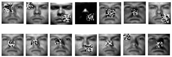
Figure 6.
Occlusion samples of one person on the Extended Yale B database.
Table 5.
Experimental results on the Extended Yale B database by using 1NN classifier and SVM classifier.
4.3. Experiments on the LFW and PubFig Databases
The Labeled Faces in the Wild database (LFW database) [46] is a challenging unconstrained face database which is collected from the Internet. It has a total of 13,233 facial images from 5749 different individuals, of which 4069 individuals only have a single image. To perform face recognition, in this section we constructed a new subset by gathering the subjects which had more than 20 samples from the original LFW database. The new subset had a total of 3023 facial images. Since these images are taken in completely real environments with non-cooperative subjects, there were complex backgrounds and some non-target subjects in the captured images. We adopted the face detection algorithm proposed in [58] to remove the interference of background and non-target subjects and croped images into 128 × 128 pixels. Some samples of one person are illustrated in Figure 7.
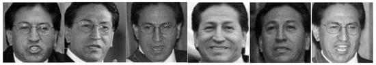
Figure 7.
Some samples of one person on the LFW database.
The PubFig database [51] is similar to the LFW database which is also collected from the Internet including 58,797 images of 200 different individuals. In our experiments, we randomly selected 99 individuals from the original database and chose 20 images of each individual to construct a new subset, of which 10 images were for training and the remaining images for testing. Similarly we also exploited the face detection method proposed in [58] to preprocess images and the size of cropped facial image was 128 × 128 pixels as shown in Figure 8.
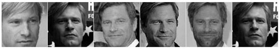
Figure 8.
Some samples of one person on the PubFig database.
In this section, we also conducted three experiments to further demonstrate the effectiveness of DSGE on two challenging facial databases. On the LFW and PubFig databases, we all randomly selected 10 images for training and reserved the remaining images for testing.
Experiment 1: We adopted PCA [10], LDA [11], NPE [23], LSDA [59], SPP [33], DSNPE [30] and our proposed DSGE for dimension reduction and exploit the SRC classifier for recognition. The recognition rate curve of each method versus the variation of dimensions is presented in Figure 9, and Table 6 lists the optimum accuracy of each method and the corresponding dimension. From them, we made observations that DSGE was always superior to the other methods regardless of the variation of dimension. More precisely, on the basis of the optimal dimension, the maximal recognition rates of DSGE on the LFW database and PubFig database were 64.84% and 37.88% respectively. It outperformed the second-placed LSDA (or LPP) by 8.54% on the LFW database, and surpassed the second-placed DSNPE by 3.53% on the PubFig database. Thus it can be seen that the performance of DSGE was not influenced by the variations of dimension and has absolute advantage in characterizing the discriminative manifold structure of unconstrained face images which are collected from completely real environments.
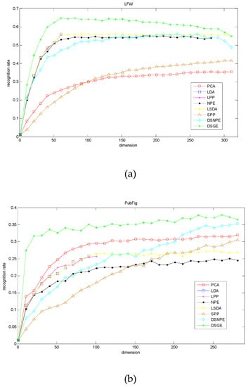
Figure 9.
Recognition rate vs. variation of dimension on the LFW database and PubFig database. (a) LFW database; (b) PubFig database.
Table 6.
The optimal recognition rates of each method and the corresponding dimension on the LFW and PubFig databases.
Experiment 2: For further evaluating the performance of DSGE on different classifiers, we also repeated the above experiment by 1NN classifier and SVM classifier respectively, in which the selected dimension of each method was identical with that in the SRC classifier as depicted in Table 6. The corresponding experimental results are presented in Table 7 and Table 8. From them, we made two observations:
Table 7.
The recognition results of different algorithms by different classifiers on the LFW database.
Table 8.
The recognition results of different algorithms by different classifiers on the PubFig database.
(1) The recognition rates of DSGE were respectively 48.94%, 60.55% and 64.84 by successively adopting 1NN classifier, SVM classifier and SRC classifier on the LFW database, which were consistently higher than those of other methods. In the same way, DSGE still outperformed the other methods regardless of which classifier is used on the PubFig database. Thereby we make conclusion that on the two challenging unconstrained face databases the performance of DSGE is not affected by the selection of classifier. Meanwhile whichever classifier is exploited, DSGE still maintains the best performance.
(2) The average value and standard deviation of recognition rates on three classifiers are shown in the last columns of Table 7 and Table 8, which can evaluate the adaptability and stability of methods on different classifiers. From them, we can see that the average recognition rate of DSGE on the LFW database is 58.11% which was the maximum, and the standard deviation of recognition rate of DSGE is 8.23% which was the minimum. Similarly, the average recognition rate of DSGE on the PubFig database is still maximal, while the standard deviation of recognition rate of DSGE is slightly higher than that of SPP. Since the average value is larger, the performance of method is more superior, conversely, the smaller the standard deviation is, the more stable the performance of method is. In view of the above results, we conclude that the performance of DSGE is not only unaffected by the selected classifier but also has better stability which does not greatly fluctuate with the classifier.
Experiment 3: Apart from the accuracy of face recognition, the computational cost is also another important issue for each method. Since these methods belonging to Sparse Graph Embedding Framework (SGEF), such as SPP, DSNPE and the proposed DSGE algorithm are all needed to construct adjacent graphs by using sparse regularization optimization algorithms [54], their computational cost is much larger than that of the classical dimensional reduction algorithms, for example PCA, LDA, LSDA, LPP and NPE. Therefore in this section we mainly discuss the computational cost of SSP, DSNPE and our proposed DSGE algorithm which include the sparse adjacent graph construction time tC and the low-dimensional projection time tP. All the experiments were conducted by using Matlab R2013a software on the 2.50 GHz Intel (R) Core (TM) i5-2450M CPU with 4GB RAM. The experimental results on the LFW database and PubFig database are listed in Table 9 respectively. We made the following observations:
Table 9.
The sparse adjacent graph construction time tc and the low-dimensional projection time tp of SPP, DSNPE and DSGE on the LFW and PubFig databases.
(1) As shown in Table 9, the low-dimensional projection time tP of SPP, DSNPE and DSGE on the LFW database and PubFig database is far less than the sparse adjacent graph construction time tC of them. For example, on the LFW database, the sparse adjacent graph construction time of SPP is 507.04 s, while the low-dimensional projection time is only 0.05 s. The value of tC is about 10,000 times as long as that of tP by SPP algorithm. Meanwhile the tC and tP of other methods also present the similar relationship. Therefore we consider that the computational complexity of SPP, DSNPE and DSGE mainly concentrates on the stage of sparse adjacent graph construction, while the running time of low-dimensional projection can be neglected.
(2) As illustrated in the last row of Table 9, the low-dimensional projection time tP of SPP, DSNPE and DSGE are fairly close, with values that fluctuate around 0.1 s on the two databases. This explains that no matter how different the theories of methods are, the running time of low-dimensional projection is similar. Hence, it is appropriate to exploit the running time of sparse adjacent graph construction to measure the computational cost of methods.
(3) Further analyzing the experimental results illustrated in the first row of Table 9, we find that the sparse adjacent graph construction time tC of DSGE is about 13 times faster than that of SPP, and is about five times faster than that of DSNPE on the LFW database. Similarly on the PubFig database, DSGE also provides the least computational complexity. The main reason is that SPP constructs the sparse adjacent graph based on the whole training samples, whereas those of DSNPE and DSGE are respectively constructed by the intra-class training samples and the inter-class training samples. Hence SPP consumes more time in contrast to DSNPE and DSGE. Meanwhile, in this paper we respectively adopt the intra-class reconstruction weight optimization algorithm and the inter-class reconstruction weight optimization algorithm (described in Section 3.1) to directly calculate the intra-class reconstruction weight and the inter-class reconstruction weight of DSGE which greatly reduces the running time of sparse adjacent graph construction. Therefore compared to DSNPE, DSGE still has competitive advantage in computational cost. In conclusion our proposed DSGE algorithm greatly reduces the computational complexity without sacrificing accuracy or quality and provides a new research idea for the following practical application.
4.4. Comparison with Deep Learning Algorithms
In the above sections we have carried out many experiments on the unconstrained face databases to demonstrate the effectiveness of our proposed method compared to the traditional subspace learning algorithms, such as LPP [22], NPE [23], SPP [33] and DSNPE [39] etc. However, as we all know, in recent years Deep Learning (DL) technology has already attracted widespread attentions due to its superior performance in many practical applications, such as face recognition [6,7], object tracking [60,61], image restoration [62,63], pose estimation [64,65], etc. Hence, in this section we also further compare the performance between DL-based algorithms and our proposed DSGE method, and analyze the advantages of using DSGE algorithm in the unconstrained face recognition. The experiments were still conducted on two challenging unconstrained face databases, i.e., LFW database and PubFig database, and the selections of training samples were identical to those in Section 4.3.
Experiment 1: For comparing with the experimental results of DL-based algorithms presented in [5] conveniently, we conducted the experiment on the PubFig 83 dataset [66] which was used in [5]. In detail, PubFig 83 dataset is the subset of PubFig database and has 13,002 face images (8720 training samples and 4282 testing samples) representing 83 individuals. In this experiment, the input data of DSGE method is the 1536-dimensional features [66] which are identical with the experimental settings of [5]. Table 10 lists the corresponding experimental results, in which the recognition rates of DeepLDA [67], Alexnet [68], VGG [69], MPDA [70] and LDA [71] are all directly quoted from [5]. We make observations that:
Table 10.
The recognition results of different methods on the PubFig 83 dataset.
(1) It is obvious that VGG achieves the highest accuracy compared to the non-DL-based algorithms, as well as the other two DL-based algorithms, i.e., Alexnet and DeepLDA. Alexnet and DeepLDA are directly trained by 8720 images, while VGG is conducted with a pre-trained model, which result in a better performance. Thus we find that DL-based algorithms need massive training samples or pre-trained model to achieve superior performance.
(2) As shown in Table 10, Alexnet and DeepLDA also perform worse than the non-deep learning methods, such as MDPA, LDA and our proposed DSGE. Especially, the recognition rate of Alexnet is 17.13% lower than that of DSGE, and the recognition rate of DeepLDA is 36.78% lower than that of DSGE. This further demonstrates that in the case of small-sample learning, DL-based algorithms have limitations. In the same way, without regard to DL-based algorithms, compared with the other two subspace learning methods, i.e., MDPA and LDA, our proposed DSGE method can still obtain the highest accuracy on the PubFig 83 dataset. Thus we conclude that our proposed DSGE method is more conducive to obtaining the discriminative manifold structure of unconstrained face images based on its improvements. Furthermore, in the condition of limited samples and limited computing resources, DSGE also can present certain advantages compared to DL-based algorithms.
Experiment 2: For further evaluating the effectiveness of DL-based features, we first adopted Histograms of Oriented Gradients (HOG) descriptor [72] and VGG [69] to extract image features of LFW and PubFig databases respectively, and then employed them into sparse graph embedding methods for unconstrained face recognition. The corresponding experimental results are shown in Table 11. From it we can see that:
Table 11.
The recognition results by introducing different feature representations into sparse graph embedding methods on the LFW and PubFig databases.
(1) Whether adopting the hand-craft features (HOG features) or the DL-based features (VGG features) into sparse graph embedding methods, i.e., SPP, DSNPE and our proposed DSGE, their recognition performances all have been significantly improved. For example, on the LFW database, the recognition rates of pixel-based methods do not exceed 70%, while those of feature-based methods all exceed 80%. Thus we conclude that the features of images are more discriminative than the original images. It is more conductive to improve the unconstrained face recognition accuracy by combining feature representations with sparse graph embedding methods.
(2) As mentioned above, the feature-based methods outperform the pixel-based methods, but there is still some performance difference between them. For example, on the PubFig database, the recognition rate of DSGE-HOG is far lower than that of DSGE-VGG, despite that it outperforms DSGE-pixels by 13.64%. Thus we find that compared to the hand-craft features, DL-based features are more accurate and more discriminative.
(3) Finally, as shown in Table 11, in the condition of adopting VGG features, our proposed DSGE still outperforms other methods. In detail, DSGE-VGG outperforms SPP-VGG and DSNPE-VGG by 0.04% and 0.37% on the LFW database, and it outperforms SPP-VGG and DSNPE-VGG by 3.43% and 0.91% on the PubFig database. Thus we conclude that DSGE still has the optimal performance.
5. Conclusions
In this paper, we propose an effective dimensionality reduction method, named Discriminative Sparse Graph Embedding (DSGE). Its improvements focus on two aspects. First, we respectively introduce the intra-class compactness constraint and inter-class compactness constraint in the procedure of adjacent graph construction for enhancing all the precision of intrinsic adjacent graph and penalty adjacent graph. Second, we respectively add the global intra-class distribution constraint and global inter-class distribution constraint into the intra-class scatter and inter-class scatter for seeking an optimal subspace in which samples in intra-classes are as compact as possible, while samples in inter-classes are as separable as possible. Thus, by combining the local neighborhood information with the global distribution information, DSGE outperforms the existing related methods on unconstrained face recognition. This conclusion is verified by extensive experiments on four face databases. In the future, we would try to introduce the feature representations into sparse subspace learning, especially DL-based features.
Author Contributions
Data curation, R.C.; Project administration, Y.T.; Writing—original draft, Y.T.; Writing—review & editing, J.Z.
Funding
This work is financially supported by the National Natural Science Foundation of China (Grant No. 61703201), NSF of Jiangsu Province (BK20170765), and NIT fund for Young Scholar (CKJB201602).
Conflicts of Interest
The authors declare no conflict of interest.
References
- Schroff, F.; Kalenichenko, D.; Philbin, J. Facenet: A unified embedding for face recognition and clustering. In Proceedings of the IEEE Conference on Computer Vision and Pattern Recognition, Boston, MA, USA, 7–12 June 2015; pp. 815–823. [Google Scholar]
- Shu, X.; Tang, J.; Li, Z.; Lai, H.; Zhang, L.; Yan, S. Personalized Age Progression with Bi-level Aging Dictionary Learning. IEEE Trans. Pattern Anal. Mach. Intell. 2018, 40, 905–917. [Google Scholar] [CrossRef]
- Shu, X.; Tang, J.; Lai, H.; Liu, L.; Yan, S. Personalized Age Progression with Aging Dictionary. In Proceedings of the IEEE International Conference on Computer Vision, Santiago, Chile, 11–18 December 2015; pp. 3970–3978. [Google Scholar]
- Yang, X.; Liu, F.; Tian, L.; Li, H.; Jiang, X. Pseudo-full-space representation based classification for robust face recognition. Signal Process. Image Commun. 2018, 60, 64–78. [Google Scholar] [CrossRef]
- Wen, J.; Fang, X.; Cui, J.; Fei, L.; Yan, K.; Chen, Y.; Xu, Y. Robust sparse linear discriminant analysis. IEEE Trans. Circuits Syst. Video Technol. 2019, 29, 390–403. [Google Scholar] [CrossRef]
- Taigman, Y.; Yang, M.; Ranzato, M.A.; Wolf, L. Deepface: Closing the gap to human-level performance in face verification. In Proceedings of the IEEE Conference on Computer Vision and Pattern Recognition, Columbus, OH, USA, 23–28 June 2014; pp. 1701–1708. [Google Scholar]
- Sun, Y.; Chen, Y.; Wang, X.; Tang, X. Deep learning face representation by joint identification-verification. In Advances in Neural Information Processing Systems; The MIT Press: Cambridge, MA, USA, 2014; pp. 1988–1996. [Google Scholar]
- Fang, X.; Han, N.; Wu, J.; Xu, Y.; Yang, J.; Wong, W.K.; Li, X. Approximate low-rank projection learning for feature extraction. IEEE Trans. Neural Netw. Learn. Syst. 2018, 29, 1–14. [Google Scholar] [CrossRef]
- Fang, X.; Teng, S.; Lai, Z.; He, Z.; Xie, S.; Wong, W.K. Robust latent subspace learning for image classification. IEEE Trans. Neural Netw. Learn. Syst. 2018, 29, 2502–2515. [Google Scholar] [CrossRef]
- Turk, M.; Pentland, A. Eigenfaces for recognition. J. Cogn. Neurosci. 1991, 3, 71–86. [Google Scholar] [CrossRef]
- Belhumeur, P.N.; Hespanha, J.P.; Kriegman, D.J. Eigenfaces vs. fisherfaces: Recognition using class specific linear projection. IEEE Trans. Pattern Anal. Mach. Intell. 1997, 19, 711–720. [Google Scholar] [CrossRef]
- Li, J.; Tao, D. Simple exponential family PCA. IEEE Trans. Neural Netw. Learn. Syst. 2013, 24, 485–497. [Google Scholar]
- Li, J.; Tao, D. On preserving original variables in Bayesian PCA with application to image analysis. IEEE Trans. Image Process. 2012, 21, 4830–4843. [Google Scholar]
- Yan, Y.; Ricci, E.; Subramanian, R.; Liu, G.; Sebe, N. Multitask linear discriminant analysis for view invariant action recognition. IEEE Trans. Image Process. 2014, 23, 5599–5611. [Google Scholar] [CrossRef]
- Seung, H.S.; Lee, D.D. The manifold ways of perception. Science 2000, 290, 2268–2269. [Google Scholar] [CrossRef]
- Zhu, B.; Liu, J.Z.; Cauley, S.F.; Rosen, B.R.; Rosen, M.S. Image reconstruction by domain-transform manifold learning. Nature 2018, 555, 487. [Google Scholar] [CrossRef]
- Ma, L.; Crawford, M.M.; Yang, X.; Guo, Y. Local-manifold-learning-based graph construction for semisupervised hyperspectral image classification. IEEE Trans. Geosci. Remote Sens. 2015, 53, 2832–2844. [Google Scholar] [CrossRef]
- Roweis, S.T.; Saul, L.K. Nonlinear dimensionality reduction by locally linear embedding. Science 2000, 290, 2323–2326. [Google Scholar] [CrossRef]
- Belkin, M.; Niyogi, P. Laplacian eigenmaps for dimensionality reduction and data representation. Neural Comput. 2003, 15, 1373–1396. [Google Scholar] [CrossRef]
- Tenenbaum, J.B.; De Silva, V.; Langford, J.C. A global geometric framework for nonlinear dimensionality reduction. Science 2000, 290, 2319–2323. [Google Scholar] [CrossRef]
- Dornaika, F.; Raduncanu, B. Out-of-sample embedding for manifold learning applied to face recognition. In Proceedings of the IEEE Conference on Computer Vision and Pattern Recognition Workshops, Portland, OR, USA, 23–28 June 2013; pp. 862–868. [Google Scholar]
- He, X.; Niyogi, P. Locality preserving projections. In Advances in Neural Information Processing Systems; The MIT Press: Cambridge, MA, USA, 2004; pp. 153–160. [Google Scholar]
- He, X.; Cai, D.; Yan, S.; Zhang, H.J. Neighborhood preserving embedding. In Proceedings of the Tenth IEEE International Conference on Computer Vision, Beijing, China, 17–20 October 2005; Volume 2, pp. 1208–1213. [Google Scholar]
- Huang, S.; Zhuang, L. Exponential Discriminant Locality Preserving Projection for face recognition. Neurocomputing 2016, 208, 373–377. [Google Scholar] [CrossRef]
- Wan, M.; Yang, G.; Gai, S.; Yang, Z. Two-dimensional discriminant locality preserving projections (2DDLPP) and its application to feature extraction via fuzzy set. Multimedia Tools Appl. 2017, 76, 355–371. [Google Scholar] [CrossRef]
- Liang, J.; Chen, C.; Yi, Y.; Xu, X.; Ding, M. Bilateral Two-Dimensional Neighborhood Preserving Discriminant Embedding for Face Recognition. IEEE Access 2017, 5, 17201–17212. [Google Scholar] [CrossRef]
- Wang, R.; Nie, F.; Hong, R.; Chang, X.; Yang, X.; Yu, W. Fast and Orthogonal Locality Preserving Projections for Dimensionality Reduction. IEEE Trans. Image Process. 2017, 26, 5019–5030. [Google Scholar] [CrossRef]
- Yan, S.; Xu, D.; Zhang, B.; Zhang, H.J.; Yang, Q.; Lin, S. Graph Embedding and Extensions: A General Framework for Dimensionality Reduction. IEEE Trans. Pattern Anal. Mach. Intell. 2007, 29, 40–51. [Google Scholar] [CrossRef]
- Sugiyama, M. Dimensionality reduction of multimodal labeled data by local fisher discriminant analysis. J. Mach. Learn. Res. 2007, 8, 1027–1061. [Google Scholar]
- Cortes, C.; Mohri, M. On transductive regression. In Advances in Neural Information Processing Systems; The MIT Press: Cambridge, MA, USA, 2007; pp. 305–312. [Google Scholar]
- Wright, J.; Yang, A.Y.; Ganesh, A.; Sastry, S.S.; Ma, Y. Robust face recognition via sparse representation. IEEE Trans. Pattern Anal. Mach. Intell. 2009, 31, 210–227. [Google Scholar] [CrossRef]
- Zhang, Z.; Xu, Y.; Yang, J.; Li, X.; Zhang, D. A survey of sparse representation: Algorithms and applications. IEEE Access 2015, 3, 490–530. [Google Scholar] [CrossRef]
- Qiao, L.; Chen, S.; Tan, X. Sparsity preserving projections with applications to face recognition. Pattern Recognit. 2010, 43, 331–341. [Google Scholar] [CrossRef]
- Lai, Z.; Mo, D.; Wen, J.; Shen, L.; Wong, W.K. Generalized robust regression for jointly sparse subspace learning. IEEE Trans. Circuits Syst. Video Technol. 2019, 29, 756–772. [Google Scholar] [CrossRef]
- Gao, Q.; Huang, Y.; Zhang, H.; Hong, X.; Li, K.; Wang, Y. Discriminative sparsity preserving projections for image recognition. Pattern Recognit. 2015, 48, 2543–2553. [Google Scholar] [CrossRef]
- Lai, Z.; Wong, W.K.; Xu, Y.; Yang, J.; Zhang, D. Approximate Orthogonal Sparse Embedding for Dimensionality Reduction. IEEE Trans. Neural Netw. Learn. Syst. 2016, 27, 723–735. [Google Scholar] [CrossRef]
- Yin, J.; Lai, Z.; Zeng, W.; Wei, L. Local sparsity preserving projection and its application to biometric recognition. Multimedia Tools Appl. 2018, 77, 1069–1092. [Google Scholar] [CrossRef]
- Zhang, Y.; Xiang, M.; Yang, B. Linear dimensionality reduction based on Hybrid structure preserving projections. Neurocomputing 2016, 173, 518–529. [Google Scholar] [CrossRef]
- Lu, G.F.; Jin, Z.; Zou, J. Face recognition using discriminant sparsity neighborhood preserving embedding. Knowl.-Based Syst. 2012, 31, 119–127. [Google Scholar] [CrossRef]
- Wei, L.; Xu, F.; Wu, A. Weighted discriminative sparsity preserving embedding for face recognition. Knowl.-Based Syst. 2014, 57, 136–145. [Google Scholar] [CrossRef]
- Lou, S.; Zhao, X.; Chuang, Y.; Yu, H.; Zhang, S. Graph Regularized Sparsity Discriminant Analysis for face recognition. Neurocomputing 2016, 173, 290–297. [Google Scholar] [CrossRef]
- Huang, K.K.; Dai, D.Q.; Ren, C.X. Regularized coplanar discriminant analysis for dimensionality reduction. Pattern Recognit. 2017, 62, 87–98. [Google Scholar] [CrossRef]
- Zhou, N.; Xu, Y.; Cheng, H.; Fang, J.; Pedrycz, W. Global and local structure preserving sparse subspace learning: An iterative approach to unsupervised feature selection. Pattern Recognit. 2016, 53, 87–101. [Google Scholar] [CrossRef]
- Liu, X.; Wang, L.; Zhang, J.; Yin, J.; Liu, H. Global and local structure preservation for feature selection. IEEE Trans. Neural Netw. Learn. Syst. 2014, 25, 1083–1095. [Google Scholar]
- Li, H.; Jiang, T.; Zhang, K. Efficient and robust feature extraction by maximum margin criterion. In Advances in Neural Information Processing Systems; The MIT Press: Cambridge, MA, USA, 2004; pp. 97–104. [Google Scholar]
- Learned-Miller, E.; Huang, G.B.; RoyChowdhury, A.; Li, H.; Hua, G. Labeled faces in the wild: A survey. In Advances in Face Detection and Facial Image Analysis; Springer International Publishing: Cham, Switzerland, 2016; pp. 189–248. [Google Scholar]
- Zhang, L.; Yang, M.; Feng, X. Sparse representation or collaborative representation: Which helps face recognition? In Proceedings of the International Conference on Computer Vision, Tokyo, Japan, 25–27 May 2011; pp. 471–478. [Google Scholar]
- Ghadimi, E.; Teixeira, A.; Shames, I.; Johansson, M. Optimal parameter selection for the alternating direction method of multipliers (ADMM): Quadratic problems. IEEE Trans. Autom. Control 2015, 60, 644–658. [Google Scholar] [CrossRef]
- AR Face Database. Available online: http://www2.ece.ohio-state.edu/~aleix/ARdatabase.html (accessed on 3 October 2015).
- Lee, K.C.; Ho, J.; Driegman, D.J. Acquiring linear subspaces for face recognition under variable lighting. IEEE Trans. Pattern Anal. Mach. Intell. 2005, 27, 684–698. [Google Scholar]
- Kumar, N.; Berg, A.C.; Belhumeur, P.N.; Nayar, S.K. Attribute and simile classifiers for face verification. In Proceedings of the IEEE International Conference on Computer Vision, Kyoto, Japan, 23–27 September 2009; pp. 365–372. [Google Scholar]
- Yin, J.; Zeng, W.; Wei, L. Optimal feature extraction methods for classification methods and their applications to biometric recognition. Knowl.-Based Syst. 2016, 99, 112–122. [Google Scholar] [CrossRef]
- Yang, J.; Chu, D.; Zhang, L.; Xu, Y.; Yang, J. Sparse representation classifier steered discriminative projection with applications to face recognition. IEEE Trans. Neural Netw. Learn. Syst. 2013, 24, 1023–1035. [Google Scholar] [CrossRef]
- Koh, K.; Kim, S.J.; Boyd, S. An interior-point method for large-scale l1-regularized logistic regression. J. Mach. Learn. Res. 2007, 8, 1519–1555. [Google Scholar]
- Wang, H.; Nie, F.; Huang, H. Robust distance metric learning via simultaneous l1-norm minimization and maximization. In Proceedings of the International Conference on Machine Learning, Beijing, China, 21–26 June 2014; pp. 1836–1844. [Google Scholar]
- Liu, Y.; Gao, Q.; Miao, S.; Gao, X.; Nie, F.; Li, Y. A non-greedy algorithm for L1-norm LDA. IEEE Trans. Image Process. 2017, 26, 684–695. [Google Scholar] [CrossRef]
- Yang, J.; Zhang, D.; Yang, J.; Niu, B. Globally maximizing, locally minimizing: Unsupervised discriminant projection with applications to face and palm biometrics. IEEE Trans. Pattern Anal. Mach. Intell. 2007, 29, 650–664. [Google Scholar] [CrossRef]
- Tong, Y.; Chen, R.; Jiao, L.; Ya, Y. An Unconstrained Face Detection Algorithm Based on Visual Saliency. In Proceedings of the International Conference on Emerging Internetworking, Data & Web Technologies, Wuhan, China, 10–11 June 2017; Springer: Cham, Switzerland, 2017; pp. 467–474. [Google Scholar]
- Cai, D.; He, X.; Zhou, K.; Han, J.; Bao, H. Locality sensitive discriminant analysis. IJCAI 2007, 2007, 1713–1726. [Google Scholar]
- Gao, J.; Zhang, T.; Yang, X.; Xu, C. P2t: Part-to-target tracking via deep regression learning. IEEE Trans. Image Process. 2018, 27, 3074–3086. [Google Scholar] [CrossRef]
- Zhai, M.; Chen, L.; Mori, G.; Javan Roshtkhari, M. Deep learning of appearance models for online object tracking. In Proceedings of the European Conference on Computer Vision, Munich, Germany, 8–14 September 2018. [Google Scholar]
- Dong, W.; Wang, P.; Yin, W.; Shi, G. Denoising prior driven deep neural network for image restoration. IEEE Trans. Pattern Anal. Mach. Intell. 2018. [Google Scholar] [CrossRef]
- Liu, P.; Zhang, H.; Zhang, K.; Lin, L.; Zuo, W. Multi-level wavelet-CNN for image restoration. In Proceedings of the IEEE Conference on Computer Vision and Pattern Recognition Workshops, Salt Lake City, UT, USA, 18–22 June 2018; pp. 773–782. [Google Scholar]
- Ranjan, R.; Patel, V.M.; Chellappa, R. Hyperface: A deep multi-task learning framework for face detection, landmark localization, pose estimation, and gender recognition. IEEE Trans. Pattern Anal. Mach. Intell. 2019, 41, 121–135. [Google Scholar] [CrossRef]
- Alp Güler, R.; Neverova, N.; Kokkinos, I. Densepose: Dense human pose estimation in the wild. In Proceedings of the IEEE Conference on Computer Vision and Pattern Recognition, Salt Lake City, UT, USA, 18–22 June 2018; pp. 7297–7306. [Google Scholar]
- Becker, B.; Ortiz, E. Evaluating open-universe face identification on the web. In Proceedings of the IEEE Conference on Computer Vision and Pattern Recognition Workshops, Portland, OR, USA, 23–28 June 2013; pp. 904–911. [Google Scholar]
- Dorfer, M.; Kelz, R.; Widmer, G. Deep linear discriminant analysis. In Proceedings of the International Conference on Learning and Representation, San Diego, CA, USA, 7–9 May 2015; pp. 1–13. [Google Scholar]
- Krizhevsky, A.; Sutskever, I.; Hinton, G.E. Imagenet classification with deep convolutional neural networks. In Advances in Neural Information Processing Systems; The MIT Press: Cambridge, MA, USA, 2012; pp. 1097–1105. [Google Scholar]
- Simonyan, K.; Zisserman, A. Very deep convolutional networks for large-scale image recognition. arXiv 2014, arXiv:1409.1556. [Google Scholar]
- Zhou, Y.; Sun, S. Manifold partition discriminant analysis. IEEE Trans. Cybern. 2017, 47, 830–840. [Google Scholar] [CrossRef]
- Martínez, A.M.; Kak, A.C. Pca versus lda. IEEE Trans. Pattern Anal. Mach. Intell. 2001, 23, 228–233. [Google Scholar] [CrossRef]
- Dalal, N.; Triggs, B. Histograms of oriented gradients for human detection. In Proceedings of the International Conference on Computer Vision & Pattern Recognition, Beijing, China, 17–20 October 2005; Volume 1, pp. 886–893. [Google Scholar]
© 2019 by the authors. Licensee MDPI, Basel, Switzerland. This article is an open access article distributed under the terms and conditions of the Creative Commons Attribution (CC BY) license (http://creativecommons.org/licenses/by/4.0/).