Online Tuning of a PID Controller with a Fuzzy Reinforcement Learning MAS for Flow Rate Control of a Desalination Unit


Abstract
:1. Introduction
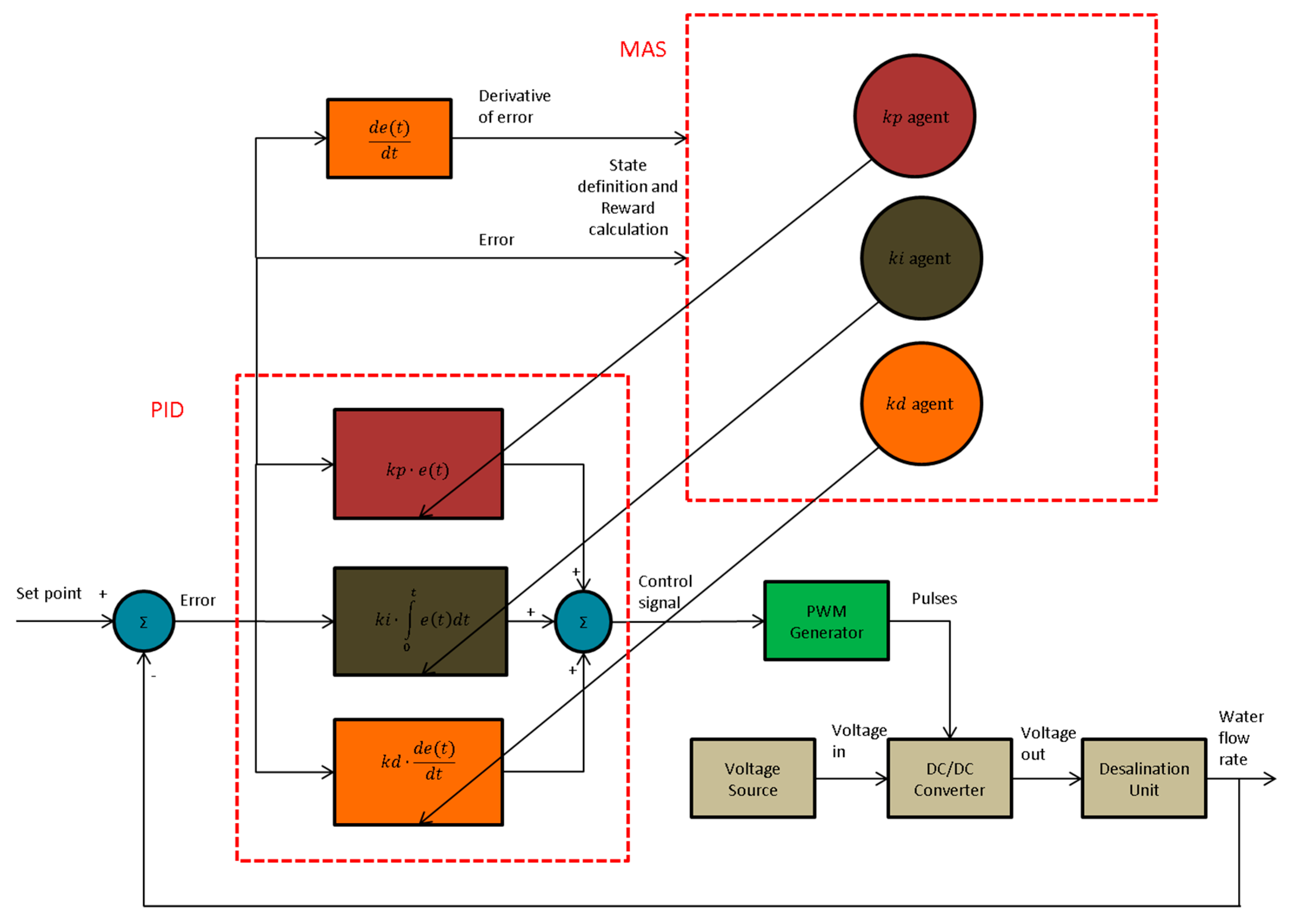
- We arrange a Q-learning MAS for adapting online the gains of a PID controller. The initial values of the gains have been set by the Z–N method.
- The PID controller is used to control the flow rate of a desalination plant. The proposed control strategy is not only independent of prior knowledge, but it is also not based on the expert’s knowledge.
- The computational resources and the implementation complexity remain low in respect to other online adaptation methods. This makes the proposed approach easy to implement.
- In order to deal with the continuous state-action space, a fuzzy logic system (FLS) is used as a fuzzy function approximator in a distributed approach.
2. Preliminaries
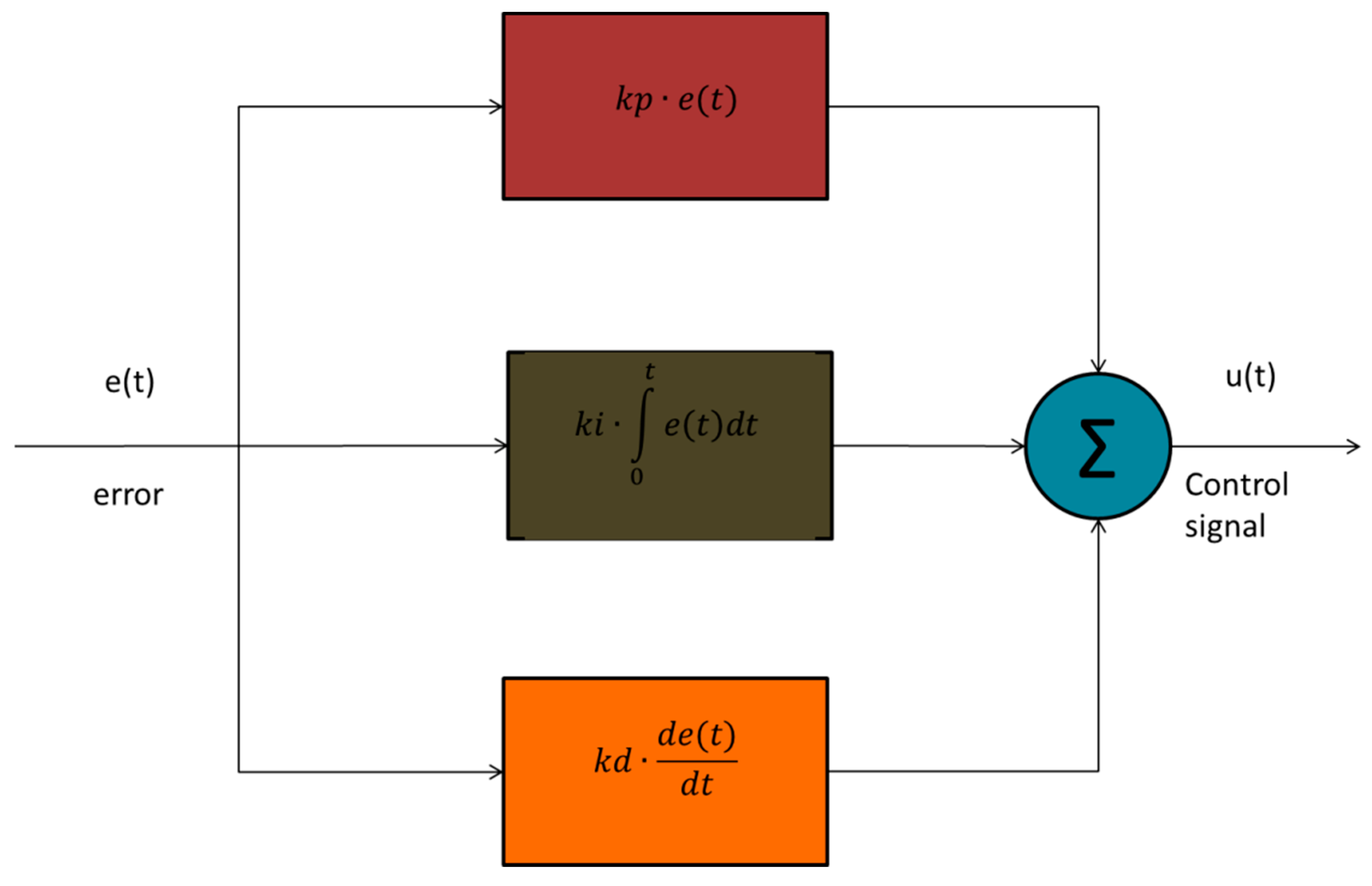
2.1. PID Controller
2.2. FLS
2.3. Reinforcement Learning
2.3.1. Q-Learning
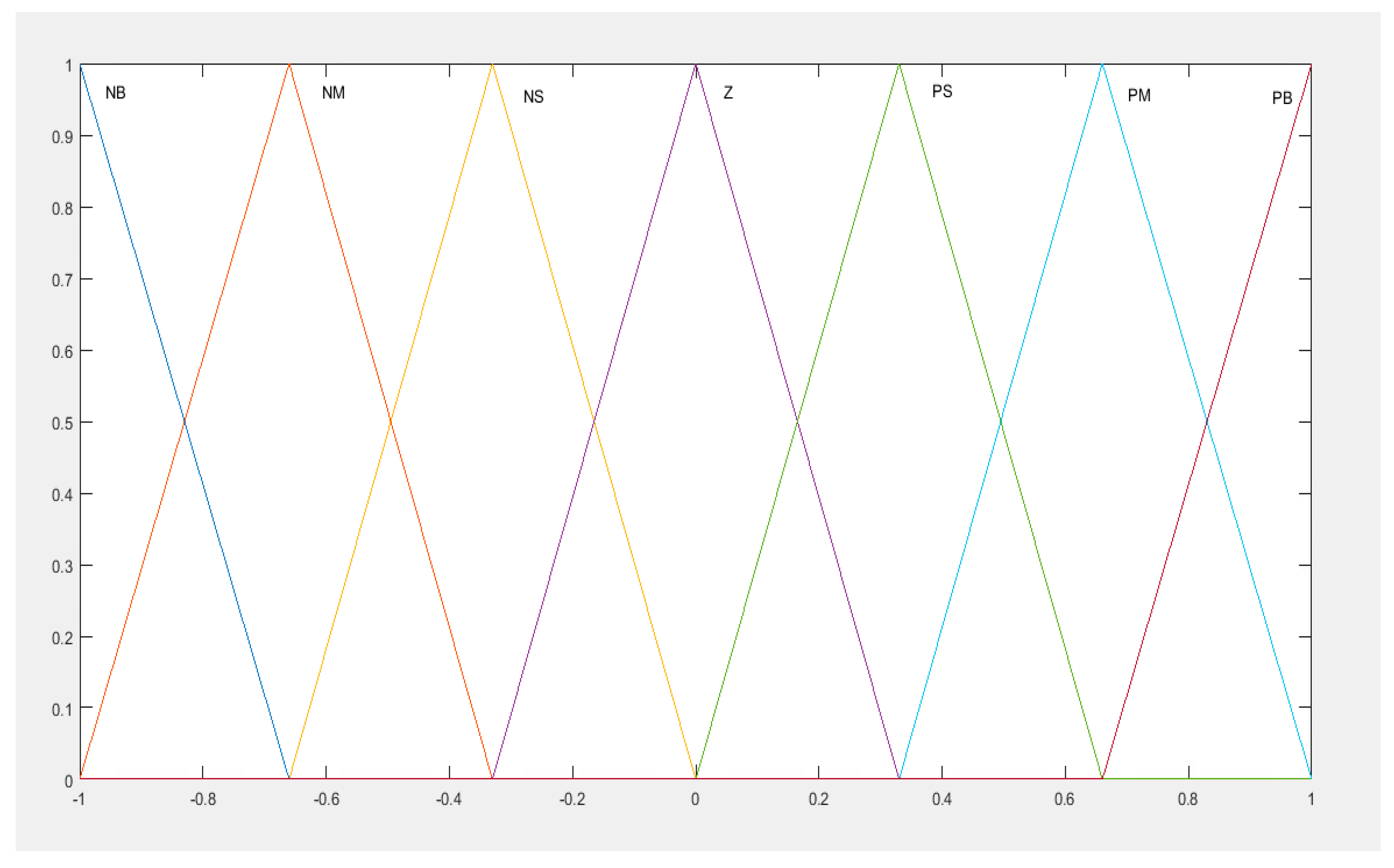
2.3.2. Fuzzy Q-Learning
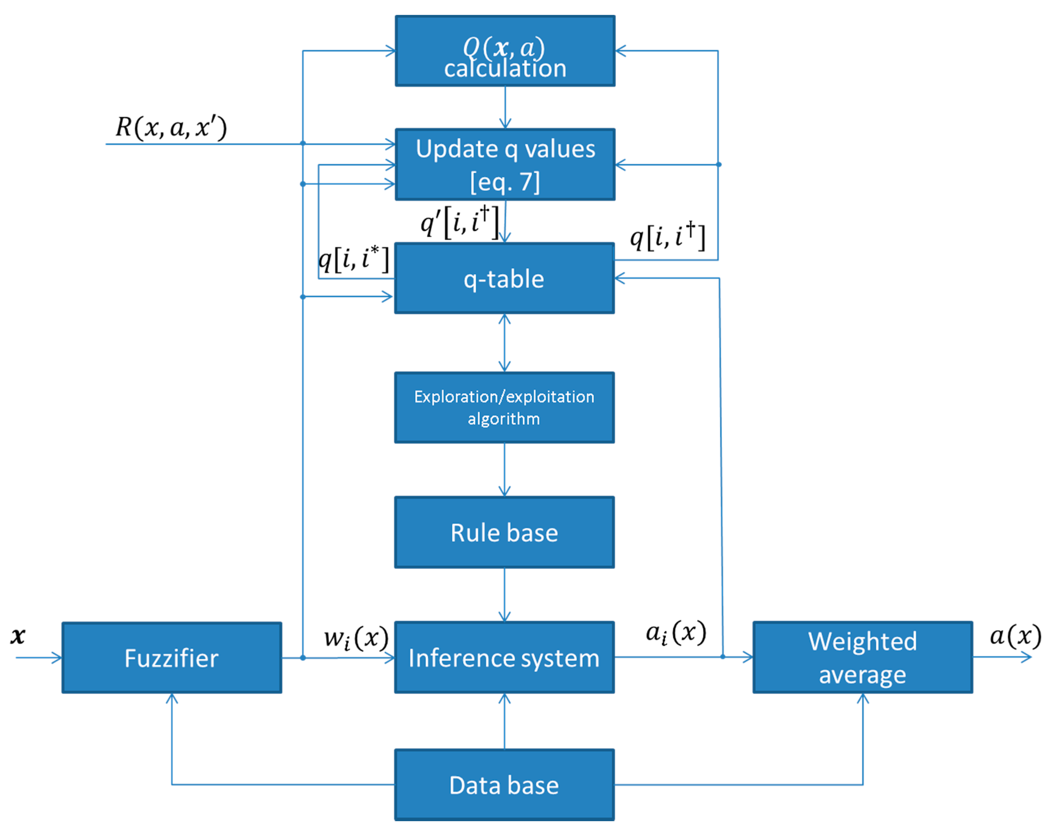
- Observe state
- Select an action for each fired rule according to the exploration/exploitation algorithm.
- Calculate the global output from the following equation:where corresponds to the chosen action of rule .
- Calculate the corresponding value as follows:where is the corresponding q-value of the fired rule for the choice of the action by the exploration/exploitation strategy.
- Apply the action and observe the new state .
- Calculate the reward
- Update the q values as follows:where and is the choice of the action that has the maximum Q value for the fired rule . The block diagram of a fuzzy Q-learning agent is depicted in Figure 2. Thus, the q values are updated as:
2.4. MAS and Q-Learning
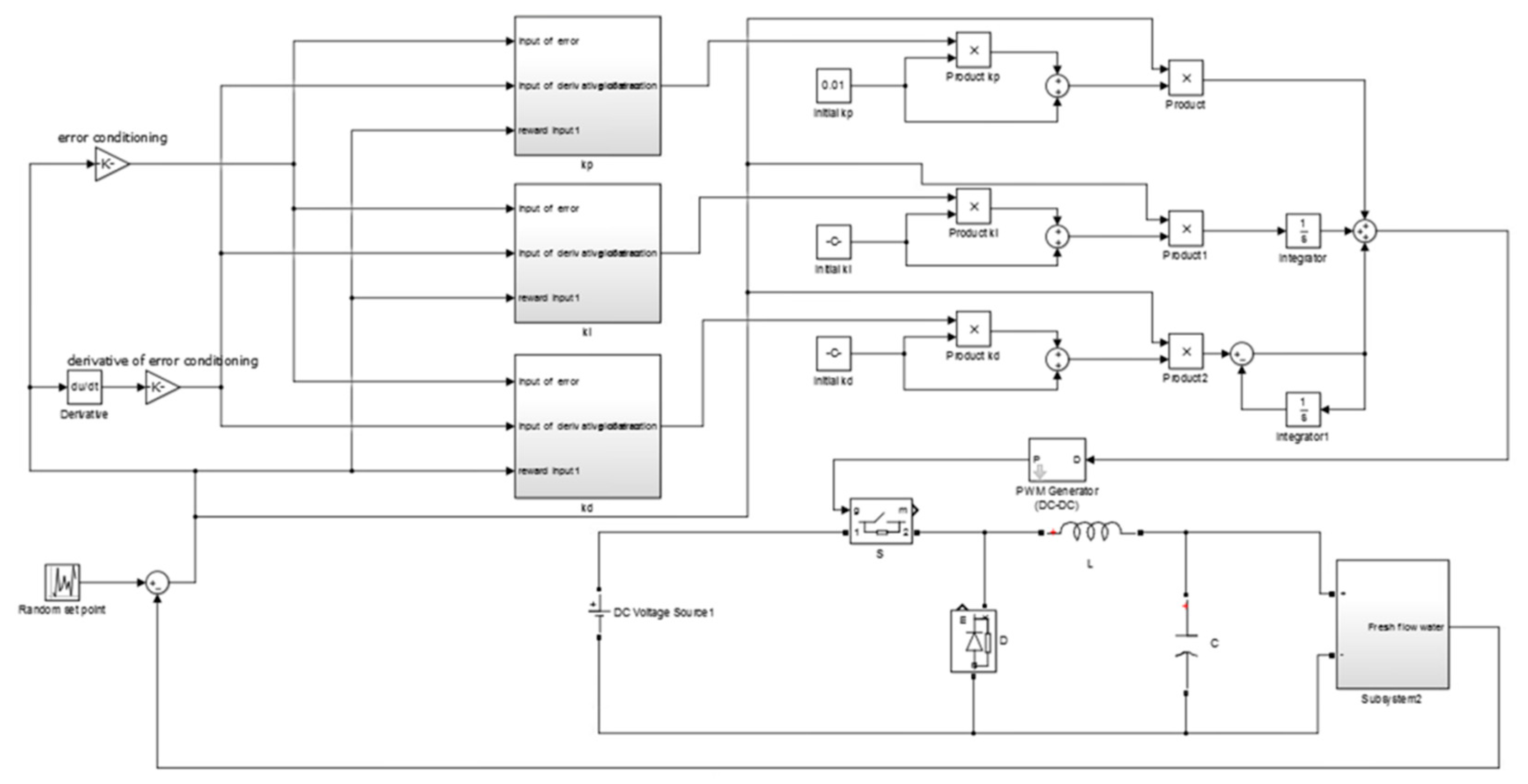
3. Desalination Model, Control Strategy and Implementation
3.1. Desalination Model
3.2. Control Strategy
3.3. Implementation
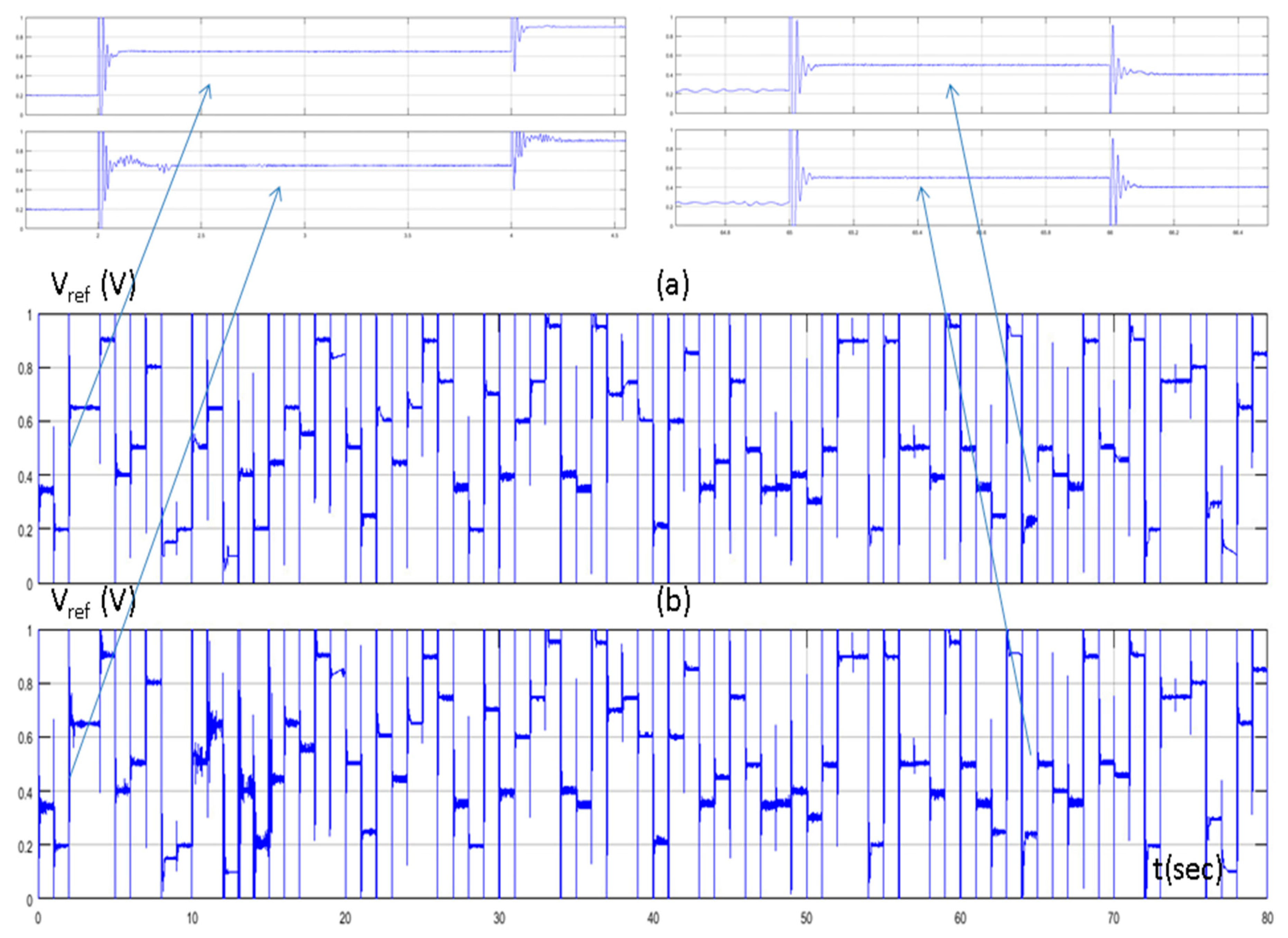
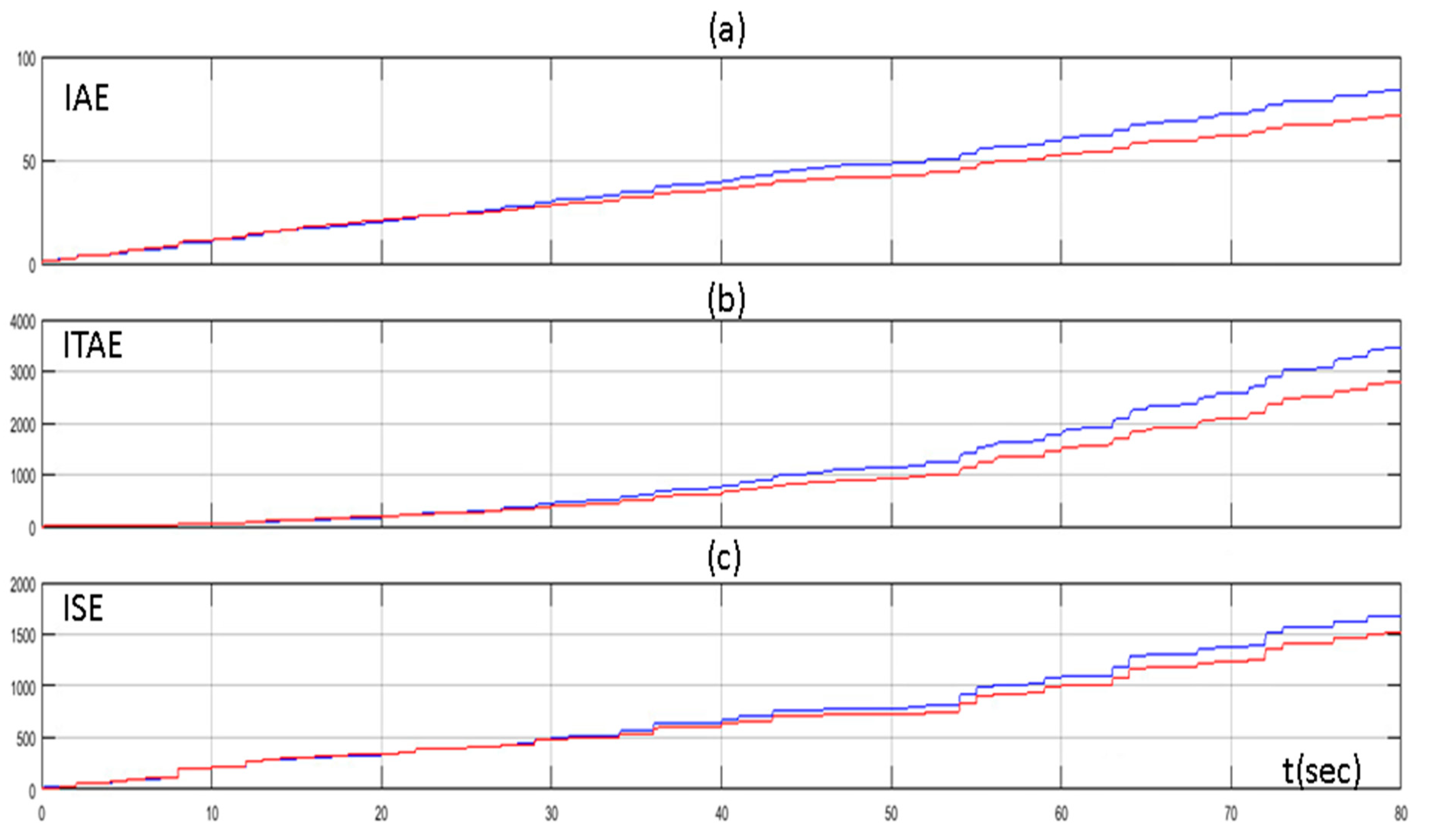
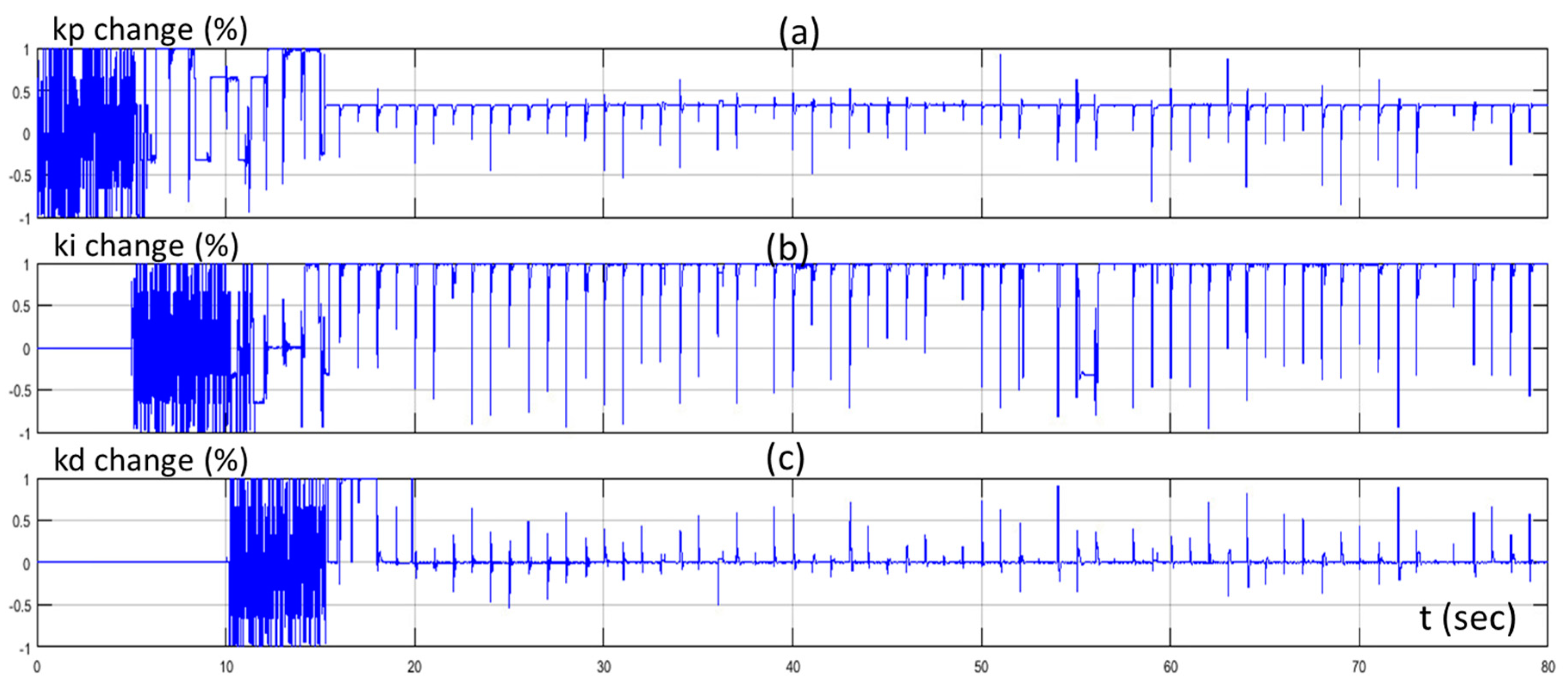
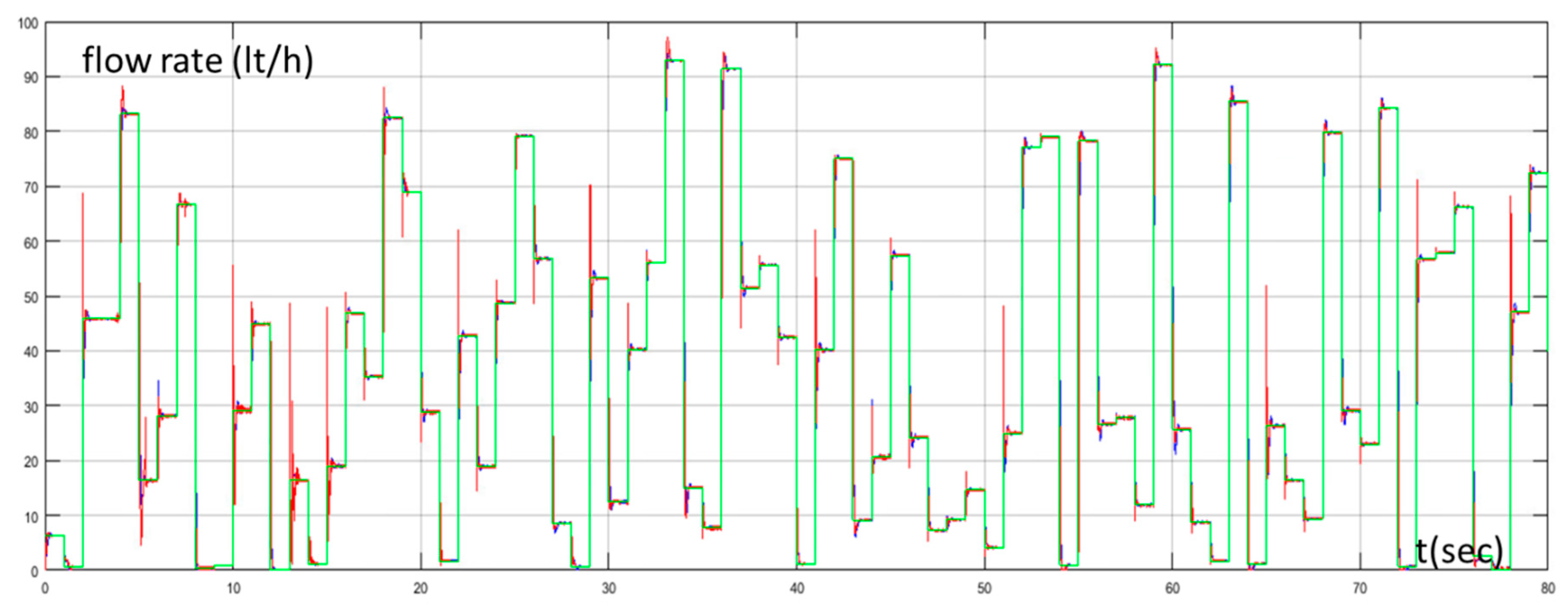
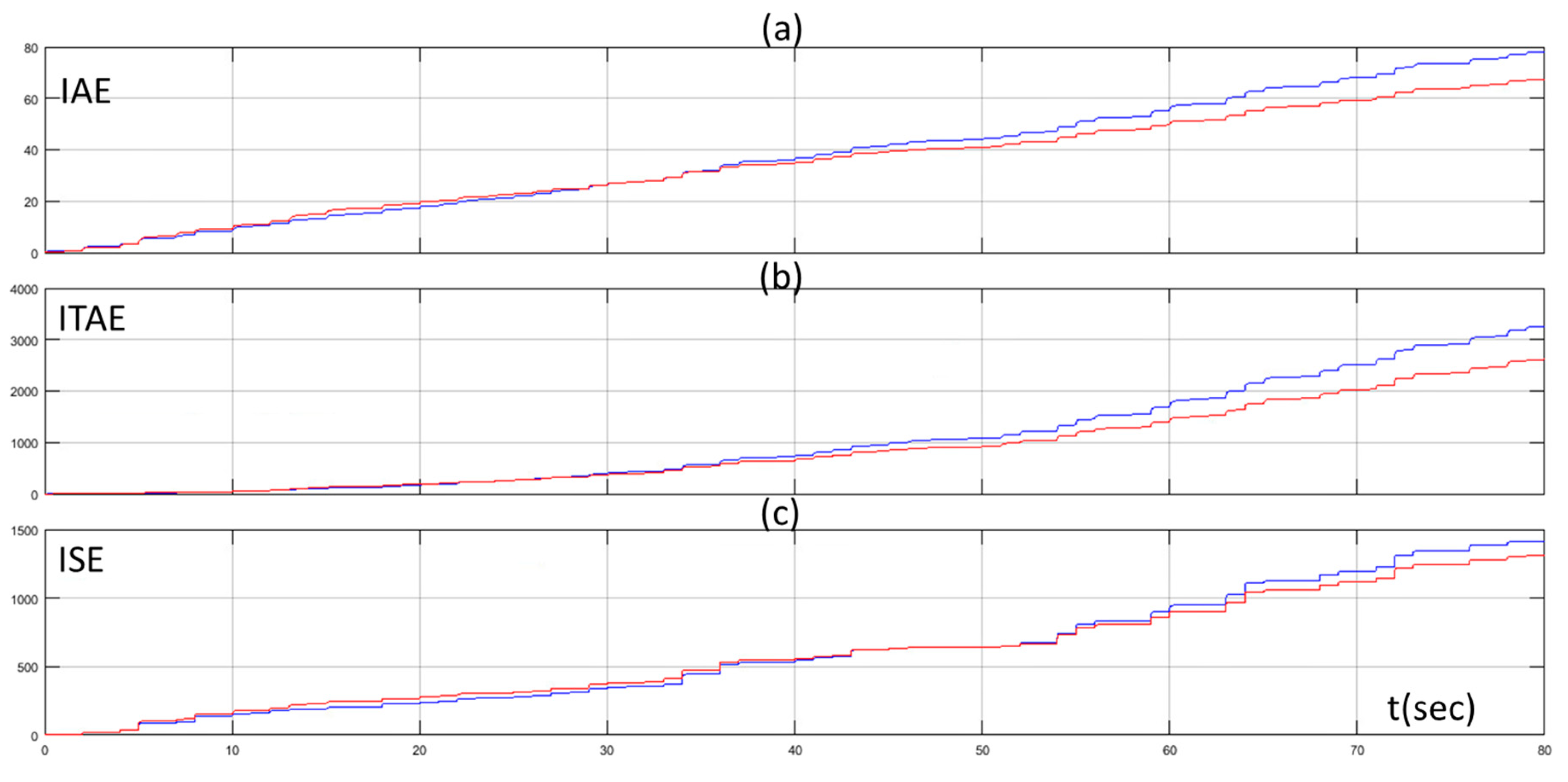
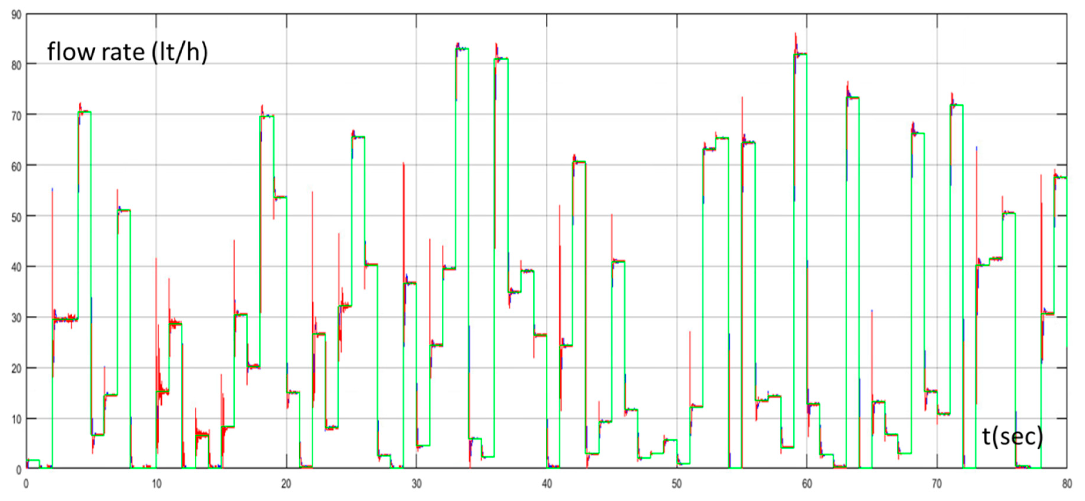
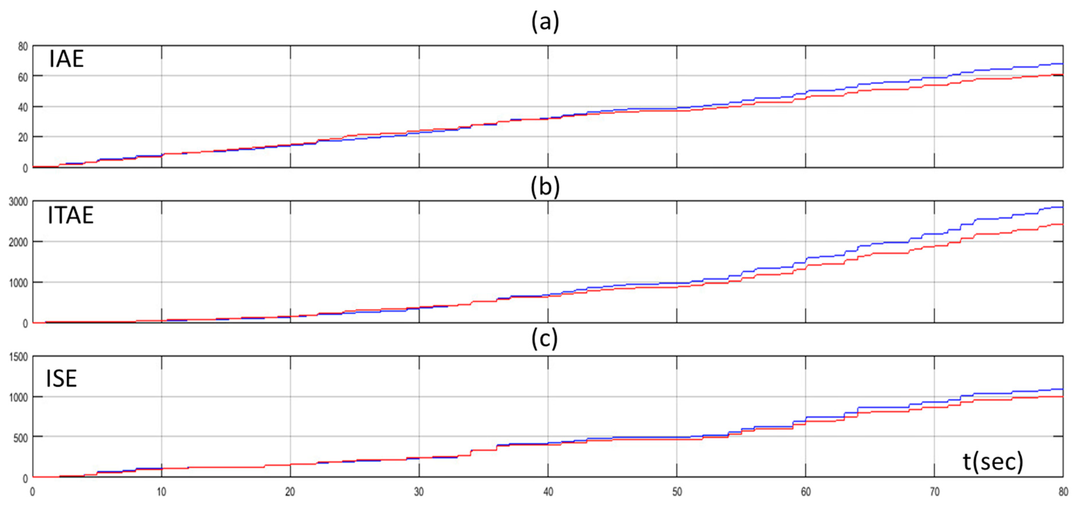
4. Simulation Results
5. Discussion
Author Contributions
Funding
Conflicts of Interest
References
- Libotean, D.; Giralt, J.; Giralt, F.; Rallo, R.; Wolfe, T.; Cohen, Y. Neural network approach for modeling the performance of reverse osmosis membrane desalting. J. Membr. Sci. 2009, 326, 408–419. [Google Scholar] [CrossRef]
- Meshram, P.M.; Kanojiya, R.G. Tuning of PID Controller using Ziegler-Nichols Method for Speed Control of DC Motor. In Proceedings of the IEEE International Conference on Advances in Engineering, Science and Management (ICAESM-2012), Nagapattinam, Tamil Nadu, India, 30–31 March 2012. [Google Scholar]
- Amaral, J.F.M.; Tanscheit, R.; Pacheco, M.A.C. Tuning PID Controllers through Genetic Algorithms. In Proceedings of the 2001 WSES International Conference on Evolutionary Computation, Puerto De La Cruz, Spain, 11–15 February 2001. [Google Scholar]
- Jayachitra, A.; Vinodha, R. Genetic Algorithm Based PID Controller Tuning Approach for Continuous Stirred Tank Reactor. Adv. Artif. Intell. 2014, 2014, 9. [Google Scholar] [CrossRef]
- Sheng, L.; Li, W. Optimization Design by Genetic Algorithm Controller for Trajectory Control of a 3-RRR Parallel Robot. Algorithms 2018, 11, 7. [Google Scholar] [CrossRef]
- Ibrahim, H.E.-S.A.; Ahmed, M.S.S.; Awad, K.M. Speed control of switched reluctance motor using genetic algorithm and ant colony based on optimizing PID controller. ITM Web Conf. 2018, 16, 01001. [Google Scholar] [CrossRef]
- Aouf, A.; Boussaid, L.; Sakly, A. A PSO algorithm applied to a PID controller for motion mobile robot in a complex dynamic environment. In Proceedings of the International Conference on Engineering & MIS (ICEMIS), Monastir, Tunisia, 8–10 May 2017. [Google Scholar]
- Ansu, E.K.; Koshy, T. Comparison of Adaptive PID controller and PSO tuned PID controller for PMSM Drives. Int. J. Adv. Eng. Res. Dev. 2018, 5, 812–820. [Google Scholar]
- Zeng, G.-Q.; Chen, J.; Dai, Y.-X.; Li, L.-M.; Zheng, C.-W.; Chen, M.-R. Design of fractional order PID controller for automatic regulator voltage system based on multi-objective extremal optimization. Neurocomputing 2015, 160, 173–184. [Google Scholar] [CrossRef]
- Abbasi, E.; Naghavi, N. Offline Auto-Tuning of a PID Controller Using Extended Classifier System (XCS) Algorithm. J. Adv. Comput. Eng. Technol. 2017, 3, 41–44. [Google Scholar]
- Muhammad, Z.; Yusoff, Z.M.; Kasuan, N.; Nordin, M.N.N.; Rahiman, M.H.F.; Taib, M.N. Online Tuning PID using Fuzzy Logic Controller with Self-Tuning Method. In Proceedings of the IEEE 3rd International Conference on System Engineering and Technology, Shah Alam, Malaysia, 19–20 August 2013. [Google Scholar]
- Dounis, A.I.; Kofinas, P.; Alafodimos, C.; Tseles, D. Adaptive fuzzy gain scheduling PID controller for maximum power point tracking of photovoltaic system. Renew. Energy 2013, 60, 202–214. [Google Scholar] [CrossRef]
- Qin, Y.; Sun, L.; Hua, Q.; Liu, P. A Fuzzy Adaptive PID Controller Design for Fuel Cell Power Plant. Sustainability 2018, 10, 2438. [Google Scholar] [CrossRef]
- Luoren, L.; Jinling, L. Research of PID Control Algorithm Based on Neural Network. Energy Procedia 2011, 13, 6988–6993. [Google Scholar]
- Badr, A.Z. Neural Network Based Adaptive PID Controller. IFAC Proc. Vol. 1997, 30, 251–257. [Google Scholar] [CrossRef]
- Rad, A.B.; Bui, T.W.; Li, Y.; Wong, Y.K. A new on-line PID tuning method using neural networks. In Proceedings of the IFAC Digital Control: Past, Present and Future of PID Control, Terrassa, Spain, 5–7 April 2000. [Google Scholar]
- Du, X.; Wang, J.; Jegatheesan, V.; Shi, G. Dissolved Oxygen Control in Activated Sludge Process Using a Neural Network-Based Adaptive PID Algorithm. Appl. Sci. 2018, 8, 261. [Google Scholar] [CrossRef]
- Agrawal, A.; Goyal, V.; Mishra, P. Adaptive Control of a Nonlinear Surge Tank-Level System Using Neural Network-Based PID Controller. In Applications of Artificial Intelligence Techniques in Engineering; Springer: Singapore, 2018; pp. 491–500. [Google Scholar]
- Hernandez-Alvarado, R.; Garcia-Valdovinos, L.G.; Salgado-Jimenez, T.; Gómez-Espinosa, A.; Navarro, F.F. Self-tuned PID Control based on Backpropagation Neural Networks for Underwater Vehicles. In Proceedings of the OCEANS 2016 MTS/IEEE, Monterey, CA, USA, 19–23 September 2016. [Google Scholar]
- Merayo, N.; Juárez, D.; Aguado, J.C.; de Miguel, I.; Durán, R.J.; Fernández, P.; Lorenzo, R.M.; Abril, E.J. PID Controller Based on a Self-Adaptive Neural Network to Ensure QoS Bandwidth Requirements in Passive Optical Networks. IEEE/OSA J. Opt. Commun. Netw. 2017, 9, 433–445. [Google Scholar] [CrossRef]
- Kim, J.-S.; Kim, J.-H.; Park, J.-M.; Park, S.-M.; Choe, W.-Y.; Heo, H. Auto Tuning PID Controller based on Improved Genetic Algorithm for Reverse Osmosis Plant. Int. J. Electron. Inf. Eng. 2008, 2, 11. [Google Scholar]
- Rathore, N.S.; Kundariya, N.; Narain, A. PID Controller Tuning in Reverse Osmosis System based on Particle Swarm Optimization. Int. J. Sci. Res. Publ. 2013, 3, 1–5. [Google Scholar]
- Jana, I.; Asuntha, A.; Brindha, A.; Selvam, K.; Srinivasan, A. Tuning of PID Controller for Reverse Osmosis (RO) Desalination System Using Particle Swarm Optimization (PSO) Technique. Int. J. Control Theory Appl. 2017, 10, 83–92. [Google Scholar]
- Glorennec, P.Y.; Jouffe, L. Fuzzy Q-learning. In Proceedings of the 6th International Fuzzy Systems Conference, Barcelona, Spain, 5 July 1997; pp. 659–662. [Google Scholar]
- Kofinas, P.; Dounis, A. Fuzzy Q-learning Agent for Online Tuning of PID Controller for DC Motor Speed Control. Algorithms 2018, 11, 148. [Google Scholar] [CrossRef]
- Kofinas, P.; Dounis, A.I.; Vouros, G.A. Fuzzy Q-learning for multi-agent decentralized energy management in microgrids. Appl. Energy 2018, 219, 53–67. [Google Scholar] [CrossRef]
- Abdulameer, A.; Sulaiman, M.; Aras, M.S.M.; Saleem, D. Tuning Methods of PID Controller for DC Motor Speed Control. Indones. J. Electr. Eng. Comput. Sci. 2016, 3, 343–349. [Google Scholar] [CrossRef]
- Tsoukalas, L.; Uhring, R. Fuzzy and Neural Approaches in Engineering; MATLAB Supplement; John Wiley & Sons: Hoboken, NJ, USA, 1997. [Google Scholar]
- Takagi, T.; Sugeno, M. Fuzzy identification of systems and its applications to modeling and control. IEEE Trans. Syst. Man Cybern. 1985, 15, 116–132. [Google Scholar] [CrossRef]
- Wang, L.-X. A Course in Fuzzy Systems and Control; Prentice Hall PTR: Upper Saddle River, NJ, USA, 1997. [Google Scholar]
- Russel, S.; Norving, P. Artificial Intelligence: A Modern Approach; Prentice Hall: Upper Saddle River, NJ, USA, 1995. [Google Scholar]
- Watkins, C.J.C.H. Learning from Delayed Reinforcement Signals. Ph.D. Thesis, University of Cambridge, Cambridge, UK, 1989. [Google Scholar]
- Sutton, R.; Barto, A. Reinforcement Learning: An Introduction; MIT Press: Cambridge, MA, USA, 1998. [Google Scholar]
- Vincent, F.S.-L.; Fonteneau, R.; Ernst, D. How to Discount Deep Reinforcement Learning: Towards New Dynamic Strategies. arXiv, 2015; arXiv:1512.02011. [Google Scholar]
- Van Hasselt, H. Reinforcement Learning in Continuous State and Action Spaces. In Reinforcement Learning: State of the Art; Springer: Berlin/Heidelberg, Germany, 2012; pp. 207–251. [Google Scholar]
- Castro, J.L. Fuzzy logic controllers are universal approximators. IEEE Trans. SMC 1995, 25, 629–635. [Google Scholar] [CrossRef]
- Sycara, K. Multiagent systems. AI Mag. 1998, 19, 79–92. [Google Scholar]
- Shi, B.; Liu, J. Decentralized control and fair load-shedding compensations to prevent cascading failures in a smart grid. Int. J. Electr. Power Energy Syst. 2015, 67, 582–590. [Google Scholar] [CrossRef]
- Puterman, M.L. Markov Decision Processes: Discrete Stochastic Dynamic Programming; Wiley: New York, NY, USA, 1994. [Google Scholar]
- Kok, J.R.; Vlassis, N. Collaborative Multiagent Reinforcement Learning by Payoff Propagation. J. Mach. Learn. Res. 2006, 7, 1789–1828. [Google Scholar]
- Claus, C.; Boutilier, C. The dynamics of reinforcement learning in cooperative multiagent systems. In Proceedings of the National Conference on Artificial Intelligence (AAAI), Madison, WI, USA, 26–30 July 1998. [Google Scholar]
- Laurent, G.J.; Matignon, L.; Fort-Piat, N.L. The world of independent learners is not markovian. KES J. 2011, 15, 55–64. [Google Scholar] [CrossRef]
- Mohamed, E.S.; Papadakis, G.; Mathioulakis, E.; Belessiotis, V. A direct-coupled photovoltaic seawater reverse osmosis desalination system toward battery-based systems—A technical and economical experimental comparative study. Desalination 2008, 221, 17–22. [Google Scholar] [CrossRef]
- Mohamed, E.S.; Papadakis, G.; Mathioulakis, E.; Belessiotis, V. An experimental comparative study of the technical and economic performance of a small reverse osmosis desalination system equipped with hydraulic energy recovery unit. Desalination 2006, 194, 239–250. [Google Scholar] [CrossRef]
- Mohamed, E.S.; Papadakis, G.; Mathioulakis, E.; Belessiotis, V. The effect of hydraulic energy recovery in a small sea water reverse osmosis desalination system; experimental and economical evaluation. Desalination 2005, 184, 241–246. [Google Scholar] [CrossRef]
- Kofinas, P.; Dounis, A.I.; Mohamed, E.S.; Papadakis, G. Adaptive neuro-fuzzy model for renewable energy powered desalination plant. Desalin. Water Treat. 2017, 65, 67–78. [Google Scholar] [CrossRef]
- Golbon, N.; Moschopoulos, G. Analysis and Design of a Higher Current ZVS-PWM Converter for Industrial Applications. Electronics 2013, 2, 94–112. [Google Scholar] [CrossRef]
- Nguyen, V.H.; Huynh, H.A.; Kim, S.Y.; Song, H. Active EMI Reduction Using Chaotic Modulation in a Buck Converter with Relaxed Output LC Filter. Electronics 2018, 7, 254. [Google Scholar] [CrossRef]


© 2019 by the authors. Licensee MDPI, Basel, Switzerland. This article is an open access article distributed under the terms and conditions of the Creative Commons Attribution (CC BY) license (http://creativecommons.org/licenses/by/4.0/).
Share and Cite
Kofinas, P.; Dounis, A.I. Online Tuning of a PID Controller with a Fuzzy Reinforcement Learning MAS for Flow Rate Control of a Desalination Unit. Electronics 2019, 8, 231. https://doi.org/10.3390/electronics8020231
Kofinas P, Dounis AI. Online Tuning of a PID Controller with a Fuzzy Reinforcement Learning MAS for Flow Rate Control of a Desalination Unit. Electronics. 2019; 8(2):231. https://doi.org/10.3390/electronics8020231
Chicago/Turabian StyleKofinas, Panagiotis, and Anastasios I. Dounis. 2019. "Online Tuning of a PID Controller with a Fuzzy Reinforcement Learning MAS for Flow Rate Control of a Desalination Unit" Electronics 8, no. 2: 231. https://doi.org/10.3390/electronics8020231
APA StyleKofinas, P., & Dounis, A. I. (2019). Online Tuning of a PID Controller with a Fuzzy Reinforcement Learning MAS for Flow Rate Control of a Desalination Unit. Electronics, 8(2), 231. https://doi.org/10.3390/electronics8020231