Finite-Time Stabilization for Stochastic Interval Systems with Time Delay and Application to Energy-Storing Electrical Circuits

Abstract

In this paper, the problem of stochastic finite-time stabilization is investigated for stochastic delay interval systems. A nonlinear state feedback controller with input-to-state delay is introduced. By employing the Lyapunov–Krasovskii functional method, some sufficient conditions on stochastic finite-time stabilization are derived for closed-loop stochastic delay interval systems using the $It\widehat{o}$’s differential formula. Suitable nonlinear state feedback controllers can be designed in terms of linear matrix inequalities. The obtained results are finally applied to an energy-storing electrical circuit to illustrate the effectiveness of the proposed method.

1. Introduction

As is well known, the feedback of real-world systems to external signals is not instantaneous as it is usually affected by a certain time delay. The time delay is an important source of oscillation, instability, and poor performance in practical systems [1,2,3,4,5]. Therefore, in the past decade, many results have been derived for linear or nonlinear uncertain time-delay systems, and a large number of papers have been published [6,7,8,9,10,11]. For example, the cooperative output regulation of discrete-time linear time-delay multi-agent systems under switching network was investigated in Reference [8]. Universal strategies to explicit adaptive control of nonlinear time-delay systems with different structures was discussed in Reference [10]. The stability and stabilization problem for time-delay systems with or without parameter uncertainties have also been addressed by many researchers [12,13,14]. An effective approach to stability and stabilization is proposed in Reference [13] for continuous-time Takagi–Sugeno fuzzy systems with time delay.

On the other hand, in real applications, parameters in a dynamical system are not always exactly known as a result of the interference of random factors. For example, in energy-storing electrical circuits, the values of capacitor C, inductor L, and resistances $R_1$ and $R_2$ are always in a certain range. Thus, it is of practical significance to study systems where the entries of a system matrix vary randomly on a certain closed interval. Such a system is called an interval system or a stochastic interval system. In recent years, stability and stabilization for stochastic delay interval systems have received increasing attention due to their extensive applications in communication networks, image processes, mobile robot localization, and so on. More recently, a large number of notable results have been reported [15,16,17,18,19,20,21,22,23]. For instance, finite-time dissipative control for stochastic interval systems with time delay and Markovian switching was studied and some sufficient matrix transformation conditions were established in Reference [17]. The robust input-to-state stability of neural networks with Markovian switching in the presence of random disturbances or time delays was studied in Reference [18]. The stability analysis of semi-Markov switched stochastic systems was introduced in Reference [20]. The finite frequency approach to controlling Markov jump linear systems with incomplete transition probabilities was investigated in Reference [23].

In addition, It is worth noting that most of the existing results on stability are focused on Lyapunov stability defined on an infinite-time interval [24,25]. Compared with Lyapunov stability, finite-time stability is such a stability property that the system states approach zero at a finite time instant rather than infinity [26,27]. It should be pointed out that finite-time stability systems might have not only faster convergence but also better robustness and disturbance rejection capabilities. Consequently, in practical applications, more attention is paid to what happens on a finite-time interval rather than an infinite-time interval. Recently, many research results on finite-time control of time-delay systems have been derived [28,29,30,31,32,33,34,35].

However, it is not difficult to see that the existing results mainly focus on the finite-time dissipative control for stochastic interval systems with time delay, or Lyapunov stability of stochastic systems with time delay. To the best of our knowledge, the problems of finite-time stability for stochastic delay interval systems have not been fully considered, which motivates this study. Meanwhile, more and more applications related to energy-storing electrical circuits are appearing everywhere playing an increasingly important part in our lives and in industrial production. Up to now, a lot of investigations on energy-storing electrical circuits have been published, e.g., finite-time control [36], stability [37], and passivity [38,39]. However, in the existing results related to energy-storing electrical circuits, the stochastic disturbance is not considered, and the values of electronic components are exact. This is almost impossible in practical energy-storing electrical circuits.

This paper aims to investigate the finite-time stabilization problem of stochastic delay interval systems. To tackle this problem, a nonlinear delay-feedback controller was used. By employing the Lyapunov–Krasovskii functional approach and $It\widehat{o}$’s differential formula, a couple of finite-time stabilization criteria were formulated such that the resulting closed-loop system was finite-time stable. Then, on the basis of the obtained criteria, suitable nonlinear delay-feedback controllers can be designed if the related linear matrix inequalities are feasible. Finally, the proposed method was applied to an energy-storing electrical circuit to demonstrate that the designed controller is effective to stabilize the energy-storing electrical circuit in finite-time. Undoubtedly, not only the error of electronic components, but also the stochastic disturbance of the energy-storing electrical circuit model proposed in this paper are considered, which means that the model proposed in this paper is more accurate and the proposed method is of considerable robustness.

The rest of this paper is organized as follow. In Section 2, we introduce some necessary system descriptions and preliminaries. The main theoretical results are derived in Section 3. An application of the proposed method to energy-storing electrical circuits is presented in Section 4, and conclusions are drawn in Section 5.

2. Systems Description and Preliminaries

Consider the following stochastic delay interval system:

$$\left\{\begin{array}{c}\mathrm{d}x\left(t\right)=[\breve{A}x\left(t\right)+{\breve{A}}_{d}x(t-\tau )+u\left(t\right)]\mathrm{d}t+[\breve{H}x\left(t\right)+{\breve{H}}_{d}x(t-\tau )]\mathrm{d}w\left(t\right),t\ge 0\hfill \\ x\left(t\right)=\phi \left(t\right),\forall t\in [-\tau ,0].\hfill \end{array}\right.$$

(1)

where $x\left(t\right)\in R^n$ is the state vector; $\tau >0$ is the time delay; $u\left(t\right)\in R^m$ is the control input; $\phi \left(t\right)\in L_2[-\tau ,0]$ is a continuous vector-valued initial function; $w\left(t\right)\in R^l$ is a scalar Brownian motion defined on the complete probability space $(\mathsf{\Omega },F,P)$ and satisfies

$$E\left\{\mathrm{d}w\left(t\right)\right\}=0,E\{\mathrm{d}w{\left(t\right)}^2\}=\mathrm{d}t.$$

In System (1), $\breve{A}$ is an interval matrix with appropriate dimension, which means

$$\breve{A}\in [\underline{A},\overline{A}]=\{\left(a_{ij}\right)\in R^{n\times n}\mid {\underline{a}}_{ij}\le a_{ij}\le {\overline{a}}_{ij},i,j=1,2,\cdots ,n\},$$

where $\underline{A}={({\underline{a}}_{ij})}_{n\times n},\overline{A}={({\overline{a}}_{ij})}_{n\times n}$ are determinate matrices. Using these matrix transformations like in Reference [17], we have

$$\breve{A}\in [\underline{A},\overline{A}]=A+△A=A+D_{1}F{G}_1$$

(2)

$${\breve{A}}_d\in [\underline{A_d},\overline{A_d}]=A_d+△A_d=A_d+D_{2}F{G}_2,$$

(3)

$$\breve{H}\in [\underline{H},\overline{H}]=H+△H=H+D_{3}F{G}_3,$$

(4)

$${\breve{H}}_d\in [\underline{H_d},\overline{H_d}]=H_d+△H_d=H_d+D_{4}F{G}_4,$$

(5)

where $F\in \overline{F}$. Let $M_1=(D_1,D_2,0,0)$, $M_2=(0,0,D_3,D_4)$, $W_1^T=(G_1^T,0,G_3^T,0)$, $W_2^T=(0,G_2^T,0,G_4^T)$. Then, (2)–(5) can be rewritten as

$$\left[\begin{array}{cc}△A& △A_d\\ △H& △H_d\end{array}\right]=\left[\begin{array}{c}{M}_1\\ M_2\end{array}\right]F\left[\begin{array}{cc}{W}_1& W_1\end{array}\right].$$

Therefore, System (1) can be rewritten as

$$\left\{\begin{array}{c}\mathrm{d}x\left(t\right)=\{[A+△A]x\left(t\right)+[A_d+△A_d]x(t-\tau )+u\left(t\right)\}\mathrm{d}t+\{[H+△H]x\left(t\right)\hfill \\ +[H_d+△H_d]x(t-\tau )\}\mathrm{d}w\left(t\right),\hfill \\ x\left(t\right)=\phi \left(t\right),\forall t\in [-\tau ,0].\hfill \end{array}\right.$$

(6)

For System (6), the desired nonlinear feedback controller is designed as follows:

$$u\left(t\right)=-Kx\left(t\right)-\overline{K}{\left|x\left(t\right)\right|}^{\alpha }sgn\left(x\left(t\right)\right)-\widehat{K}{({\int }_{t-\tau }^{t}x{\left(s\right)}^{T}x\left(s\right)\mathrm{d}s)}^{\frac{1+\alpha }{2}}(\frac{\left|x\right(t\left)\right|}{{\parallel x\left(t\right)\parallel }^2}),$$

(7)

where $0<\alpha <1$; $K,\overline{K},\widehat{K}$ are real matrices; $x_i\left(t\right)\in R^n,i=1,2,\dots ,n$, $sgn\left(x\left(t\right)\right)=diag(sgn\left(x_1\left(t\right)\right)$, $sgn\left(x_2\left(t\right)\right),\dots ,sgn\left(x_n\left(t\right)\right){)}^T$.

Remark 1.

In fact, the control gain matrices $K,\overline{K},\widehat{K}$ in the controller $u\left(t\right)$ play different roles in ensuring the stochastic finite-time stability of System (6), where K is used to keep the Lyapunov–Krasovskii stability of (6). Furthermore, the convergence of finite-time stability of (6) to zero is determined by $\overline{K}$. Finally, the influence of time-delay term on the systems is eliminated by $\widehat{K}$.

Remark 2.

In order to break the Lipschitz condition, the parameter α is defined in $0<\alpha <1$. On the contrary, when $\alpha \le 0$ or $\alpha \ge 1$, there exists a unique solution for the systems, which contradicts the definition of finite-time stability. Therefore, the parameter α must be in $0<\alpha <1$.

In this paper, we mainly consider the finite-time stabilization of System (6). To begin with, we introduce the following definitions and lemmas:

Definition 1 (Stochastic Settling Time Function (SSTF)).

For SDISs (6), define $T_0(x_0,\omega )=inf\{T\ge 0:x(t,x_0)=0,\forall t\ge T\}$, which is called the stochastic settling time function, especially, $T_0(x_0,\omega )=\infty$, if $x(t,x_0)\ne 0,\forall t>0$.

Definition 2 (Stochastic Finite-Time Stability (SFTS)).

The origin $x=0$ of System (1) or (6) are said to the stochastic finite-time stability, if the following two conditions hold:

(i) 

The origin of System (6) is stochastic stability in probability.

(ii) 

The origin of System (6) is stochastic finite-time convergent (SFTC), i.e., for any initial conditions $\varphi \left(s\right)\in \mathsf{\Lambda },$ the SSTF $T_0(x_0,\omega )$ exists, that is $E\left\{T_0(x_0,\omega )\right\}<\infty ,$ for $\forall \in R^n\backslash \left\{0\right\}$.

Definition 3.

System (6) is stochastic finite-time stable if there exists a feedback controller $u\left(t\right)$, such that the controlled System (6) is SFTS.

Lemma 1

([40]). Assume that System (6) has a unique global solution. If there exists a positive-definite, two continuous differentiable and radially unbounded Lyapunov function $V:R^n\to R_{+}$ and a continuous differentiable function $\gamma :R_{+}\to R_{+}$ such that

(i) 

$\ell V\left(x\right)\le -\gamma \left(V\right(x\left)\right),$

(ii) 

for any $0\le \epsilon \le +\infty ,{\int }_0^{\epsilon }\frac{1}{\gamma \left(v\right)}\mathrm{d}v<+\infty ,$

(iii) 

for $v>0,{\gamma }^{\prime }\left(v\right)>0,$

then the origin solution of (6) is SFST, and the SSTF $T_0(x_0,\omega )$ satisfies $E\left[T_0(x_0,\omega )\right]\le {\int }_0^{V\left(x_0\right)}\frac{1}{\gamma \left(v\right)}\mathrm{d}v$, which implies $T_0(x_0,\omega )<\infty$, a.s.

Lemma 2

([41]). Assume that System (6) admits a unique solution. If there exists a $C^2$ function $V:R^n\to R^{+},K_{\infty }$ class function ${\mu }_1$ and ${\mu }_2$, positive real constant $c>0$ and $0<r<1,$ such that for all $x\in R^n$ and $t\ge 0$,

$${\mu }_1\left(\right|x\left|\right)\le V\left(x\right)\le {\mu }_2\left(\right|x\left|\right),$$

$$\ell V\left(x\right)\le -c{\left(V\left(x\right)\right)}^r,$$

then the origin solution of (6) is SFTS.

Lemma 3

([42]). For given matrices $Q=Q^T$, H and E with appropriate dimensions,

$$Q+HF\left(t\right)E+E^{T}F{\left(t\right)}^T{H}^T<0,$$

holds for all $F{\left(t\right)}^{T}F\left(t\right)\le I$ if and only if there exists $\epsilon >0$ such that

$$Q+{\epsilon }^{-1}H{H}^T+\epsilon E^{T}E<0.$$

Lemma 4

([43]). ($It\widehat{o}$ formula) Let $x\left(t\right)$ be an n-dimensional $It\widehat{o}$ Process on $t\ge 0$ with the stochastic differential

$$\mathrm{d}x\left(t\right)=f\left(t\right)\mathrm{d}t+g\left(t\right)\mathrm{d}B\left(t\right).$$

Let $V\in C^{2,1}(R^n\times R_{+};R).$ Then, $V\left(x\right(t),t)$ is a real valued $It\widehat{o}$ process with its stochastic differential given by

$$\mathrm{d}V(x\left(t\right),t)=\ell V(x\left(t\right),t)\mathrm{d}t+V_x(x\left(t\right),t)g\left(t\right)\mathrm{d}B\left(t\right).$$

where $\ell V(x\left(t\right),t)=V_t(x\left(t\right),t)+V_x(x\left(t\right),t)f\left(t\right)+\frac{1}{2}trace\left(g^T\left(t\right)V_{xx}(x\left(t\right),t)g\left(t\right)\right)$.

3. Finite-Time Stabilization for Stochastic Delay Interval Systems

Theorem 1.

If there exist a real matrix Y, and a symmetric positive-definite matrix X, some positive constants ${\epsilon }_1,{\epsilon }_2,{\epsilon }_3>0$ such that

$$\left[\begin{array}{cccc}{\mathsf{{\rm Y}}}_1& A_{d}X& H^T& {\mathsf{{\rm Y}}}_3\\ *& -X& H_d^T& {\mathsf{{\rm Y}}}_4\\ *& *& {\mathsf{{\rm Y}}}_2& 0\\ *& *& *& {\mathsf{{\rm Y}}}_5\end{array}\right]<0$$

(8)

where

• ${\mathsf{{\rm Y}}}_1=X{A}^T+AX+{\epsilon }_1{D}_1{D}_1^T+{\epsilon }_2{D}_2{D}_2^T-Y^T-Y+X,$
• ${\mathsf{{\rm Y}}}_2=-X+{\epsilon }_3(D_3{D}_3^T+D_4{D}_4^T),$
• ${\mathsf{{\rm Y}}}_3=(G_1^T,0,G_3^T,0),$
• ${\mathsf{{\rm Y}}}_4=(0,G_2^T,0,G_4^T),$
• ${\mathsf{{\rm Y}}}_5=diag(-{\epsilon }_{1}I,-{\epsilon }_{2}I,-{\epsilon }_{3}I,-{\epsilon }_{3}I),$

then the close-loop control system (6) is finite-time stabilizable. In this case, the parameters of the controller are given as $K=Y{X}^{-1},{\overline{K}}^T\overline{K}>0,{\widehat{K}}^T\widehat{K}>0$, and the setting-time function can be estimated by $E\left[T_0(x_0,\omega )\right]\le \frac{{\lambda }_{max}\left(P\right){\parallel x\left(0\right)\parallel }^{1-\alpha }}{c(1-\alpha )}$ with $c=2max\{\sqrt{{\lambda }_{max}({\overline{K}}^T\overline{K})},\sqrt{{\lambda }_{max}({\widehat{K}}^T\widehat{K})}\}.$

Proof. 

Construct the following Lyapunov–Krasovskii functional candidate as

$$V\left(x\left(t\right)\right)=x{\left(t\right)}^{T}Px\left(t\right)+{\int }_{t-\tau }^{t}x{\left(s\right)}^{T}Px\left(s\right)\mathrm{d}s.$$

(9)

From $It\widehat{o}$ formula of Lemma 4, we have

$$\mathrm{d}V\left(x\left(t\right)\right)=\ell V\left(x\right)\mathrm{d}t+2x{\left(t\right)}^{T}P[H+△H]x\left(t\right)+[H_d+△H_d]x(t-\tau )]\mathrm{d}w\left(t\right).$$

(10)

By means of $It\widehat{o}$ formula, one has

$$\begin{array}{c}\ell V\left(x\right)=2{\{[A+△A]x\left(t\right)+[A_d+△A_d]x(t-\tau )+u\left(t\right)\}}^{T}Px\left(t\right)+\{[H+△H]\times \hfill \\ \hspace{1em}\hspace{1em}\hspace{1em}x\left(t\right)+[H_d+△H_d]x(t-\tau ){\}}^{T}P\{[H+△H]x\left(t\right)+[H_d+△H_d]x(t-\tau )\}+\hfill \\ \hspace{1em}\hspace{1em}\hspace{1em}x{\left(t\right)}^{T}Px\left(t\right)-x{(t-\tau )}^{T}Px(t-\tau )\hfill \\ \hspace{1em}\hspace{1em}=2\{[A+△A]x\left(t\right)+[A_d+△A_d]x(t-\tau )-Kx\left(t\right)-\overline{K}|x\left(t\right){|}^{\alpha }sgn\left(x\left(t\right)\right)-\hfill \\ \hspace{1em}\hspace{1em}\hspace{1em}\widehat{K}{({\int }_{t-\tau }^{t}x{\left(s\right)}^{T}x\left(s\right)\mathrm{d}s)}^{\frac{1+\alpha }{2}}(\frac{\left|x\right(t\left)\right|}{{\parallel x\left(t\right)\parallel }^2}){\}}^{T}Px\left(t\right)+\{[H+△H]x\left(t\right)+\hfill \\ \hspace{1em}\hspace{1em}\hspace{1em}[H_d+△H_d]x(t-\tau ){\}}^{T}P\{[H+△H]x\left(t\right)+[H_d+△H_d]\times \hfill \\ \hspace{1em}\hspace{1em}\hspace{1em}{x(t-\tau )\}+x\left(t\right)}^{T}Px\left(t\right)-x{(t-\tau )}^{T}Px(t-\tau ).\hfill \end{array}$$

(11)

By using Lemma 3, we can get

$$\begin{array}{c}{(△Ax\left(t\right)+△A_{d}x(t-\tau ))}^{T}Px\left(t\right)+x{\left(t\right)}^{T}P(△Ax\left(t\right)+△A_{d}x(t-\tau ))\hfill \\ =(x{\left(t\right)}^T{G}_1^{T}F\left(t\right)D_1^T+x{(t-\tau )}^T{G}_2^{T}F\left(t\right)D_2^T)Px\left(t\right)+\hfill \\ x{\left(t\right)}^{T}P(D_{1}F\left(t\right)G_{1}x\left(t\right)+D_{2}F\left(t\right)G_{2}x(t-\tau ))\hfill \\ =x{\left(t\right)}^T(P{D}_{1}F\left(t\right)G_1+G_1^{T}F\left(t\right)D_1^{T}P)x\left(t\right)+\hfill \\ x{\left(t\right)}^{T}P{D}_{2}F\left(t\right)G_{2}x(t-\tau )+x{(t-\tau )}^T{G}_2^{T}F\left(t\right)D_2^{T}Px\left(t\right)\hfill \\ \le x\left(t\right)({\epsilon }_1^{-1}{G}_1^T{G}_1+{\epsilon }_{1}P{D}_1{D}_1^{T}P)x{\left(t\right)}^T+\hfill \\ {\epsilon }_{2}x{\left(t\right)}^{T}P{D}_2{D}_2^{T}Px\left(t\right)+{\epsilon }_2^{-1}x{(t-\tau )}^T{G}_2^T{G}_{2}x(t-\tau )).\hfill \end{array}$$

(12)

Hence, (11) can be written as

$$\begin{array}{c}\ell V\left(x\right)={\left(\begin{array}{c}{x}_t^T\\ x{(t-\tau )}^T\end{array}\right)}^T\mathsf{\Sigma }\left(\begin{array}{c}{x}_t\\ x(t-\tau )\end{array}\right)-2\overline{K}{\left|x\left(t\right)\right|}^{\alpha }sgn\left(x\left(t\right)\right)Px\left(t\right)-\hfill \\ \hspace{1em}\hspace{1em}\hspace{1em}2\widehat{K}{({\int }_{t-\tau }^{t}x{\left(s\right)}^{T}x\left(s\right)\mathrm{d}s)}^{\frac{1+\alpha }{2}}(\frac{\left|x\right(t\left)\right|}{{\parallel x\left(t\right)\parallel }^2})Px\left(t\right),\hfill \end{array}$$

(13)

where

$$\begin{array}{cc}\hfill \mathsf{\Sigma }=& \left[\begin{array}{cc}{\mathsf{\Psi }}_{11}& P{A}_d\\ *& {\mathsf{\Psi }}_{22}\end{array}\right]+\left(\begin{array}{c}{H}^T+△H^T\\ H_d^T+△H_d^T\end{array}\right)P\left(\begin{array}{cc}H+△H& H_d+△H_d\end{array}\right),\hfill \\ \hfill {\mathsf{\Psi }}_{11}=& A^{T}P+PA-K^{T}P-PK+P+{\epsilon }_1^{-1}{G}_1^T{G}_1+{\epsilon }_{1}P{D}_1{D}_1^{T}P+{\epsilon }_{2}P{D}_2{D}_2^{T}P,\hfill \\ \hfill {\mathsf{\Psi }}_{22}=& -P+{\epsilon }_2^{-1}{G}_2^T{G}_2.\hfill \end{array}$$

By the Schur complement, we have

$$\mathsf{\Sigma }<0\iff \left[\begin{array}{ccc}{\mathsf{\Psi }}_{11}& P{A}_d& H^T+△H^T\\ *& {\mathsf{\Psi }}_{22}& H_d^T+△H_d^T\\ *& *& -P^{-1}\end{array}\right]=\left[\begin{array}{ccc}{\mathsf{\Psi }}_{11}& P{A}_d& H^T\\ *& {\mathsf{\Psi }}_{22}& H_d^T\\ *& *& -P^{-1}\end{array}\right]+\left[\begin{array}{ccc}0& 0& △H^T\\ 0& 0& △H_d^T\\ *& *& 0\end{array}\right]<0.$$

(14)

Applying Lemma 3, we have that $\mathsf{\Sigma }<0$ is equivalent to the following matrix inequality

$$\left[\begin{array}{cccc}{\mathsf{{\rm Y}}}_1& A_{d}X& H^T& {\mathsf{{\rm Y}}}_3\\ *& -X& H_d^T& {\mathsf{{\rm Y}}}_4\\ *& *& {\mathsf{{\rm Y}}}_2& 0\\ *& *& *& {\mathsf{{\rm Y}}}_5\end{array}\right]<0,$$

(15)

where

• ${\mathsf{{\rm Y}}}_1=X{A}^T+AX+{\epsilon }_1{D}_1{D}_1^T+{\epsilon }_2{D}_2{D}_2^T-Y^T-Y+X,$
• ${\mathsf{{\rm Y}}}_2=-X+{\epsilon }_3(D_3{D}_3^T+D_4{D}_4^T),$
• ${\mathsf{{\rm Y}}}_3=(G_1^T,0,G_3^T,0),$
• ${\mathsf{{\rm Y}}}_4=(0,G_2^T,0,G_4^T),$
• ${\mathsf{{\rm Y}}}_5=diag(-{\epsilon }_{1}I,-{\epsilon }_{2}I,-{\epsilon }_{3}I,-{\epsilon }_{3}I.$

Set $J=(X,X,I,I,I,I)$ with $P^{-1}=X$ and $KX=Y$. Multiplying by $J^T$ and J, respectively, on both sides of the matrix in (15), by the Schur complement, we readily obtain (8) from (15).

On the other hand, it follows directly from (11) that

$$\begin{array}{c}\ell V\left(x\right)\le -2c_1{\left|x\left(t\right)\right|}^{\alpha }sgn\left(x\left(t\right)\right)Px\left(t\right)-2c_2{({\int }_{t-\tau }^{t}x{\left(s\right)}^{T}x\left(s\right)\mathrm{d}s)}^{\frac{1+\alpha }{2}}(\frac{\left|x\right(t\left)\right|}{{\parallel x\left(t\right)\parallel }^2})Px\left(t\right)\hfill \\ \hspace{1em}\hspace{1em} \le -2max\{c_1,c_2\}V{\left(x\left(t\right)\right)}^{\frac{1+\alpha }{2}}\hfill \\ \hspace{1em}\hspace{1em} \le -cV{\left(x\left(t\right)\right)}^{\frac{1+\alpha }{2}},\hfill \end{array}$$

(16)

where $c_1=\sqrt{{\lambda }_{max}({\overline{K}}^T\overline{K})},$ $c_2=\sqrt{{\lambda }_{max}({\widehat{K}}^T\widehat{K})},$ $c=2max\{c_1,c_2\}$. Thus, according to Lemma 1, the system (6) is SFTS via the nonlinear delay-feedback controller (7). Moreover, from Lemma 1, the SSTF satisfies

$$\begin{array}{c}E\left\{T_0(x_0,\omega )\right\}\le {\int }_0^{V\left(x_0\right)}\frac{1}{cV{\left(x\left(t\right)\right)}^{\frac{1+\alpha }{2}}}\mathrm{d}v\hfill \\ \hspace{1em}\hspace{1em}\hspace{1em}\hspace{1em}\hspace{1em}\le \frac{V{\left(x_0\right)}^{\frac{1-\alpha }{2}}}{c(1-\alpha )}\hfill \\ \hspace{1em}\hspace{1em}\hspace{1em}\hspace{1em}\hspace{1em}\le \frac{{\lambda }_{max}\left(P\right){\parallel x\left(0\right)\parallel }^{1-\alpha }}{c(1-\alpha )}.\hfill \end{array}$$

(17)

The proof is completed. □

Remark 3.

In the proof of Theorem 1, the specific Lyapunov–Krasovskii function is determined by the particularity of the controller. In order to reduce the conservatism of the controller, minor changes are made to the controller. Therefore, it is as follows:

$$u(t)=-Kx\left(t\right)-\overline{K}{\left|x\left(t\right)\right|}^{\alpha }sgn\left(x\left(t\right)\right)-\widehat{K}{({\int }_{t-\tau }^{t}x{\left(s\right)}^{T}Qx\left(s\right)\mathrm{d}s)}^{\frac{1+\alpha }{2}}(\frac{P^{-1}\left|x\left(t\right)\right|}{{\parallel x\left(t\right)\parallel }^2}),$$

(18)

where $0<\alpha <1$, $K,\overline{K},\widehat{K},P^{-1},Q$ are real matrices, $x_i\left(t\right)\in R^n,i=1,2,\dots ,n$, $sgn\left(x\left(t\right)\right)=diag(sgn\left(x_1\left(t\right)\right)$, $sgn\left(x_2\left(t\right)\right),\dots ,sgn\left(x_n\left(t\right)\right){)}^T$.

Theorem 2.

For the given ${\epsilon }_1,{\epsilon }_2,{\epsilon }_3>0$, if there exist a real matrix Y and a symmetric positive-definite matrix X such that

$$\mathsf{\Pi }=\left[\begin{array}{cccc}{\Phi }_1& A_{d}X& H^T& {\Phi }_3\\ *& \tilde{Q}& H_d^T& {\Phi }_4\\ *& *& {\Phi }_2& 0\\ *& *& *& {\Phi }_5\end{array}\right]<0,$$

(19)

where

• ${\mathsf{\Phi }}_1=X{A}^T+AX+{\epsilon }_1{D}_1{D}_1^T+{\epsilon }_2{D}_2{D}_2^T-Y^T-Y+\tilde{Q},$
• ${\mathsf{\Phi }}_2=-X+{\epsilon }_3(D_3{D}_3^T+D_4{D}_4^T),$
• ${\mathsf{\Phi }}_3=(G_1^T,0,G_3^T,0),$
• ${\mathsf{\Phi }}_4=(0,G_2^T,0,G_4^T),$
• ${\mathsf{\Phi }}_5=diag(-{\epsilon }_{1}I,-{\epsilon }_{2}I,-{\epsilon }_{3}I,-{\epsilon }_{3}I).$
• $\tilde{Q}=-XQX.$

then the close-loop control system (6) is finite-time stabilizable. In this case, the parameters of the controller are given as $K=Y{X}^{-1},{\overline{K}}^T\overline{K}>0,{\widehat{K}}^T\widehat{K}>0$, and the setting-time function can be estimated by $E\left[T_0(x_0,\omega )\right]\le \frac{{\lambda }_{max}\left(P\right){\parallel x\left(0\right)\parallel }^{1-\alpha }}{c(1-\alpha )}$ with $c=2max\{\sqrt{{\lambda }_{max}({\overline{K}}^T\overline{K})},\sqrt{{\lambda }_{max}({\widehat{K}}^T\widehat{K})}\}.$

Proof. 

Construct the Lyapunov–Krasovskii functional as follows:

$$V\left(x\left(t\right)\right)=x{\left(t\right)}^{T}Px\left(t\right)+{\int }_{t-\tau }^{t}x{\left(s\right)}^{T}Qx\left(s\right)\mathrm{d}s.$$

(20)

It can be derived by $It\widehat{o}$ formula that

$$\mathrm{d}V(x(t))=\ell V\left(x\right)\mathrm{d}t+2x{\left(t\right)}^{T}P[H+△H]x\left(t\right)+[H_d+△H_d]x(t-\tau )]\mathrm{d}w\left(t\right),$$

(21)

where

$$\begin{array}{c}\ell V\left(x\right)=2{\{[A+△A]x\left(t\right)+[A_d+△A_d]x(t-\tau )+u\left(t\right)\}}^{T}Px\left(t\right)+\left\{\right[H+\hfill \\ \hspace{1em}\hspace{1em}\hspace{1em}△H]x\left(t\right)+[H_d+△H_d]x(t-\tau ){\}}^{T}P\{[H+△H]x\left(t\right)+\hfill \\ \hspace{1em}\hspace{1em}\hspace{1em}[H_d+△H_d]x(t-\tau )\}+x{\left(t\right)}^{T}Qx\left(t\right)-x{(t-\tau )}^{T}Qx(t-\tau )\hfill \\ \hspace{1em}\hspace{1em} =2\{[A+△A]x\left(t\right)+[A_d+△A_d]x(t-\tau )-Kx\left(t\right)-\overline{K}|x\left(t\right){|}^{\alpha }sgn\left(x\left(t\right)\right)-\hfill \\ \hspace{1em}\hspace{1em}\hspace{1em}\widehat{K}{({\int }_{t-\tau }^{t}x{\left(s\right)}^{T}Qx\left(s\right)\mathrm{d}s)}^{\frac{1+\alpha }{2}}(\frac{P^{-1}\left|x\left(t\right)\right|}{{\parallel x\left(t\right)\parallel }^2}){\}}^{T}Px\left(t\right)+\{[H+△H]x\left(t\right)+\hfill \\ \hspace{1em}\hspace{1em}\hspace{1em}[H_d+△H_d]x(t-\tau ){\}}^{T}P\{[H+△H]x\left(t\right)+[H_d+△H_d]x(t-\tau )\}+\hfill \\ \hspace{1em}\hspace{1em}\hspace{1em}x{\left(t\right)}^{T}Qx\left(t\right)-x{(t-\tau )}^{T}Qx(t-\tau )\hfill \\ \hspace{1em}\hspace{1em} ={\left(\begin{array}{c}{x}_t^T\\ x{(t-\tau )}^T\end{array}\right)}^T\mathsf{\Pi }\left(\begin{array}{c}{x}_t\\ x(t-\tau )\end{array}\right)-2\overline{K}{\left|x\left(t\right)\right|}^{\alpha }sgn\left(x\left(t\right)\right)Px\left(t\right)-\hfill \\ \hspace{1em}\hspace{1em}\hspace{1em}2\widehat{K}{({\int }_{t-\tau }^{t}x{\left(s\right)}^{T}Qx\left(s\right)\mathrm{d}s)}^{\frac{1+\alpha }{2}}(\frac{P^{-1}\left|x\left(t\right)\right|}{{\parallel x\left(t\right)\parallel }^2})Px\left(t\right).\hfill \end{array}$$

(22)

On the basis of Theorem 2, we know that $\mathsf{\Pi }<0$. So, we can get

$$\begin{array}{c}\ell V\left(x\right)\le -2c_1{\left|x\left(t\right)\right|}^{\alpha }sgn\left(x\left(t\right)\right)Px\left(t\right)-\hfill \\ \hspace{1em}\hspace{1em}\hspace{1em} 2c_2{({\int }_{t-\tau }^{t}x{\left(s\right)}^{T}Qx\left(s\right)\mathrm{d}s)}^{\frac{1+\alpha }{2}}(\frac{P^{-1}\left|x\left(t\right)\right|}{{\parallel x\left(t\right)\parallel }^2})Px\left(t\right)\hfill \\ \hspace{1em}\hspace{1em} \le -2max\{c_1,c_2\}V{\left(x\left(t\right)\right)}^{\frac{1+\alpha }{2}}\hfill \\ \hspace{1em}\hspace{1em} \le -cV{\left(x\left(t\right)\right)}^{\frac{1+\alpha }{2}},\hfill \end{array}$$

(23)

here $c_1=\sqrt{{\lambda }_{max}({\overline{K}}^T\overline{K})},$ $c_2=\sqrt{{\lambda }_{max}({\widehat{K}}^T\widehat{K})},$ $c=2max\{c_1,c_2\},$ Thus, according to Lemma 1, the SDISs (6) are SFTS via the nonlinear delay-feedback controller (18). Furthermore, from Lemma 1, the SSTF satisfies

$$\begin{array}{c}E\left\{T_0(x_0,\omega )\right\}\le {\int }_0^{V\left(x_0\right)}\frac{1}{cV{\left(x\left(t\right)\right)}^{\frac{1+\alpha }{2}}}\mathrm{d}v\hfill \\ \hspace{1em}\hspace{1em}\hspace{1em}\hspace{1em}\hspace{1em}\le \frac{V{\left(x_0\right)}^{\frac{1-\alpha }{2}}}{c(1-\alpha )}\hfill \\ \hspace{1em}\hspace{1em}\hspace{1em}\hspace{1em}\hspace{1em}\le \frac{{\lambda }_{max}\left(P\right){\parallel x\left(0\right)\parallel }^{1-\alpha }}{c(1-\alpha )}.\hfill \end{array}$$

(24)

The proof is completed. □

4. Application to the Energy-Storing Electrical Circuit

In this section, as an application of above results on finite-time stability, we consider an energy storage circuit.

Figure 1 shows an energy-storing electrical circuit, which includes power source E, capacitors C, inductor L, and resistance $R_1,R_2$. There is only one capacitor connected in the circuit. In this circuit, when the power supply voltage is E and the switch S is turned off, the capacitive element begins to store energy, and the inductor also begins to replenish energy, and finally reaches stability. However, it is impossible to get the exact value of the capacitor C, inductor L, and resistances $R_1,R_2$ in practical application, but the approximate value is available. Assuming the capacitor C, inductor L, and resistances $R_1,R_2$ are linear and time invariant, and the exact value of the capacitor, inductor, and resistances are $C,L,R_1,R_2$, respectively. Whilst at the same time, the measured value are $C\pm △C$, $L\pm △L$, $R_1\pm △R_1$, $R_2\pm △R_2$. Then, we can model them as

$$\begin{array}{cc}\hfill \frac{\mathrm{d}{U}_C}{\mathrm{d}t}=& \frac{1}{C\pm △C}{i}_C,\hfill \\ \hfill \frac{\mathrm{d}{i}_L}{\mathrm{d}t}=& \frac{1}{L\pm △L}{U}_C,\hfill \end{array}$$

(25)

where, i and U denote the electric current and the electric tension across an element.

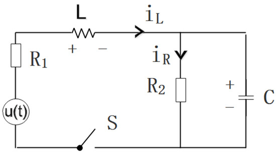
Figure 1. Energy-storing electrical circuit.

Taking $x_1\left(t\right)=U_C\left(t\right)$ and $x_2\left(t\right)=i_L\left(t\right)$ as the state variables, $u\left(t\right)=E$ as the excitation. According to the basic electrical circuits laws, we have

$$\begin{array}{c}{\dot{x}}_1\left(t\right)=\frac{1}{C\pm △C}[-\frac{x_1\left(t\right)}{R_2\pm △R_2}+x_2\left(t\right)],\hfill \\ {\dot{x}}_2\left(t\right)=\frac{1}{L\pm △L}[-x_1\left(t\right)-(R_1\pm △R_1)x_2\left(t\right)+u\left(t\right)].\hfill \end{array}$$

(26)

When the switch S is closed, System (26) can be written as

$$\left\{\begin{array}{c}\dot{x}\left(t\right)=\breve{A}x\left(t\right)+\breve{B}u\left(t\right),\hfill \\ x\left(t_0\right)=x_0,\hfill \end{array}\right.$$

(27)

where

$$\breve{A}=\left[\begin{array}{cc}-\frac{1}{(C\pm △C)(R_2\pm △R_2)}& \frac{1}{C\pm △C}\\ -\frac{1}{L\pm △L}& -\frac{R_1\pm △R_1}{L\pm △L}\end{array}\right],\breve{B}=\left[\begin{array}{c}0\\ \frac{1}{L\pm △L}\end{array}\right].$$

It is well known that a time delay is inescapable in modeling systems, which is very common in manual control, nuclear, reactor, and communication networks. It may lead to instability and oscillation. Undoubtedly, in the energy-storing electrical circuit illustrated in Figure 1, a time delay is inevitable. Meanwhile, if we pay attention to the structural uncertainty, stochastic disturbance must be considered. Therefore, the above systems can be written as

$$\left\{\begin{array}{c}\mathrm{d}x\left(t\right)=[\breve{A}x\left(t\right)+{\breve{A}}_{d}x(t-\tau )+\breve{B}u\left(t\right)]\mathrm{d}t+[\breve{H}x\left(t\right)+{\breve{H}}_{d}x(t-\tau )]\mathrm{d}w\left(t\right)\hfill \\ x\left(t_0\right)=x_0,\hfill \end{array}\right.$$

(28)

where $x\left(t\right)\in R^n$ is the state vector; $\tau >0$ is the time delay; $u\left(t\right)\in R^m$ is the control input; $w\left(t\right)\in R^l$ is a scalar Brownian motion defined on the complete probability space $(\mathsf{\Omega },F,P)$ and satisfies

$$E\left\{\mathrm{d}w\left(t\right)\right\}=0,E\{\mathrm{d}w{\left(t\right)}^2\}=\mathrm{d}t.$$

Similar to the matrix transformation of System (1), System (28) can be rewritten as

$$\left\{\begin{array}{c}\mathrm{d}x\left(t\right)=\{[A+△A]x\left(t\right)+[A_d+△A_d]x(t-\tau )+[B+△B]u\left(t\right)\}\mathrm{d}t+\left\{\right[H+\hfill \\ △H]x\left(t\right)+[H_d+△H_d]x(t-\tau )\}\mathrm{d}w\left(t\right)\hfill \\ x\left(t_0\right)=x_0.\hfill \end{array}\right.$$

(29)

Thus, the nonlinear delay-feedback controller is as follows:

$$u(t)=-Kx\left(t\right)-\overline{K}{\left|x\left(t\right)\right|}^{\alpha }sgn\left(x\left(t\right)\right)-\widehat{K}{({\int }_{t-\tau }^{t}x{\left(s\right)}^{T}Qx\left(s\right)\mathrm{d}s)}^{\frac{1+\alpha }{2}}(\frac{P^{-1}\left|x\left(t\right)\right|}{{\parallel x\left(t\right)\parallel }^2}),$$

(30)

where $0<\alpha <1$, $K,\overline{K},\widehat{K},P^{-1},Q$ are real matrices, $x\left(t\right)={(x_1\left(t\right),x_2\left(t\right),\dots ,x_n\left(t\right))}^T$∈Rⁿ, $sgn\left(x\left(t\right)\right)=diag{(sgn\left(x_1\right)\left(t\right),sgn\left(x_2\left(t\right)\right),\dots ,sgn\left(x_n\left(t\right)\right))}^T$.

4.1. A Criterion on Finite-Time Stabilization

Theorem 3.

For the given ${\epsilon }_1,{\epsilon }_2,{\epsilon }_3,{\epsilon }_4>0$, if there exist a real matrix Y, and a symmetric positive-definite matrix X such that

$$\mathsf{\Xi }=\left[\begin{array}{cccc}{\mathsf{\Xi }}_1& A_{d}X& H^T& {\mathsf{\Xi }}_3\\ *& -\tilde{Q}& H_d^T& {\mathsf{\Xi }}_4\\ *& *& {\mathsf{\Xi }}_2& 0\\ *& *& *& {\mathsf{\Xi }}_5\end{array}\right]<0,$$

(31)

where

• ${\mathsf{\Xi }}_1=X{A}^T+AX+{\epsilon }_1{D}_1{D}_1^T+{\epsilon }_2{D}_2{D}_2^T-{\epsilon }_4{D}_5{D}_5^T-Y^T{B}^T-BY+\tilde{Q},$
• ${\mathsf{\Xi }}_2=-X+{\epsilon }_3(D_3{D}_3^T+D_4{D}_4^T),$
• ${\mathsf{\Xi }}_3=(G_1^T,0,G_3^T,0,-Y^T{G}_5^T),$
• ${\mathsf{\Xi }}_4=(0,G_2^T,0,G_4^T,0),$
• ${\mathsf{\Xi }}_5=diag(-{\epsilon }_{1}I,-{\epsilon }_{2}I,-{\epsilon }_{3}I,-{\epsilon }_{3}I,-{\epsilon }_{4}I).$
• $\tilde{Q}=XQX,$

then the close-loop control system (29) is finite-time stabilizable. In this case, the parameters of the controller are given as $K=Y{X}^{-1},K_1^T{K}_1>0,K_2^T{K}_2>0$, and the setting-time function can be estimated by $E\left[T_0(x_0,\omega )\right]\le \frac{{\lambda }_{max}\left(P\right){\parallel x\left(0\right)\parallel }^{1-\alpha }}{c(1-\alpha )}$ with $c=2max\{\sqrt{{\lambda }_{max}(K_1^T{K}_1)},\sqrt{{\lambda }_{max}(K_2^T{K}_2)}\}$.

Proof. 

Construct the following Lyapunov–Krasovskii functional as follows:

$$V\left(x\left(t\right)\right)=x{\left(t\right)}^{T}Px\left(t\right)+{\int }_{t-\tau }^{t}x{\left(s\right)}^{T}Qx\left(s\right)\mathrm{d}s.$$

(32)

Similar to the proof of Theorem 2, we can get

$$\begin{array}{c}\ell V(x)\le -2[B+△B]\overline{K}{\left|x\left(t\right)\right|}^{\alpha }sgn\left(x\left(t\right)\right)Px\left(t\right)-2[B+△B]\widehat{K}{({\int }_{t-\tau }^{t}x{\left(s\right)}^{T}Qx\left(s\right)\mathrm{d}s)}^{\frac{1+\alpha }{2}}(\frac{P^{-1}\left|x\left(t\right)\right|}{{\parallel x\left(t\right)\parallel }^2})Px\left(t\right)\hfill \\ \hspace{1em}\hspace{1em} \le -2c_3{\left|x\left(t\right)\right|}^{\alpha }sgn\left(x\left(t\right)\right)Px\left(t\right)-2c_4{({\int }_{t-\tau }^{t}x{\left(s\right)}^{T}Qx\left(s\right)\mathrm{d}s)}^{\frac{1+\alpha }{2}}(\frac{P^{-1}\left|x\left(t\right)\right|}{{\parallel x\left(t\right)\parallel }^2})Px\left(t\right)\hfill \\ \hspace{1em}\hspace{1em} \le -2max\{c_3,c_4\}V{\left(x\left(t\right)\right)}^{\frac{1+\alpha }{2}}\hfill \\ \hspace{1em}\hspace{1em} \le -cV{\left(x\left(t\right)\right)}^{\frac{1+\alpha }{2}},\hfill \end{array}$$

(33)

where $K_1={\overline{K}}^T{B}^T+B\overline{K}+{\epsilon }_4{D}_5{D}_5^T+{\epsilon }_4^{-1}{G}_5\overline{K}{\overline{K}}^T{G}_5^T$, $K_2={\widehat{K}}^T{B}^T+B\widehat{K}+{\epsilon }_4{D}_5{D}_5^T+{\epsilon }_4^{-1}{G}_5\widehat{K}{\widehat{K}}^T{G}_5^T$, $c_3=\sqrt{{\lambda }_{max}(K_1^T{K}_1)},$$c_4=\sqrt{{\lambda }_{max}(K_2^T{K}_2)},$ $c=2max\{c_3,c_4\}.$ Thus, according to Lemma 1, System (29) is SFTS. Furthermore, from Lemma 1, the SSTF satisfies

$$\begin{array}{c}E\{T_0(x_0,\omega )\}\le {\int }_0^{V\left(x_0\right)}\frac{1}{cV{\left(x\left(t\right)\right)}^{\frac{1+\alpha }{2}}}\mathrm{d}v\hfill \\ \hspace{1em}\hspace{1em}\hspace{1em}\hspace{1em}\hspace{1em}\le \frac{V{\left(x_0\right)}^{\frac{1-\alpha }{2}}}{c(1-\alpha )}\hfill \\ \hspace{1em}\hspace{1em}\hspace{1em}\hspace{1em}\hspace{1em}\le \frac{{\lambda }_{max}\left(P\right){\parallel x\left(0\right)\parallel }^{1-\alpha }}{c(1-\alpha )}.\hfill \end{array}$$

(34)

The proof is completed. □

Remark 4.

To design an appropriate controller (30) for stochastic energy-storing electrical circuit (29), that is to determine $K,\overline{K},\widehat{K}$, an algorithm is given as follows:

(1) 

For the given parameters in stochastic energy-storing electrical circuit (29), calculate $D_i,G_i,i=1,2,3,4$.

(2) 

Solve LMI (31), get the positive matrices $X,Y$, and calculate $K=Y{X}^{-1}$.

(3) 

Choose appropriate matrices $\overline{K}$ and $\widehat{K}$, such that $K_1^T{K}_1>0$ and $K_2^T{K}_2>0$.

(4) 

Calculate $V\left(0\right)$, and determine the upper bounded of stochastic settling time function $E\left\{T_0(x_0,\omega )\right\}\le \frac{{\lambda }_{max}\left(P\right){\parallel x\left(0\right)\parallel }^{1-\alpha }}{c(1-\alpha )}.$

4.2. Simulations

For the energy storage circuit in Figure 1, suppose that $C=6\times {10}^3\mathsf{\mu }\mathrm{F},\Delta C=0.2\times {10}^3\mathsf{\mu }\mathrm{F},L=0.2\mathrm{H},\Delta L=0.01\mathrm{H},R_1=1\mathsf{\Omega },\Delta R_1=0.01\mathsf{\Omega },R_2=800\mathsf{\Omega },\Delta R_2=10\mathsf{\Omega }.$ According to (27) and (28), we can get

$$\begin{array}{c}\hfill \breve{A}=\left[\begin{array}{cc}[-0.2182,-0.1991]& [161.2903,172.4138]\\ [-5.2632,-4.7619]& [-52.6842,-47.57143]\end{array}\right],\breve{B}=\left[\begin{array}{cc}0.1& 0\\ 0& [4.7619,5.2632]\end{array}\right].\end{array}$$

Then, we set $\tau =0.5,T=5$$x\left(0\right)={[-12]}^T$ and

$$\begin{array}{c}\hfill \breve{A_d}=\left[\begin{array}{cc}[-0.32,-0.10]& [11.30,12.11]\\ 1& [-50.34,-40.57]\end{array}\right],\breve{H}=\left[\begin{array}{cc}[0.1,0.2]& [1,1.2]\\ [-1,1.5]& [1,1.5]\end{array}\right],\breve{H_d}=\left[\begin{array}{cc}[1,1.5]& [0,1]\\ [-1,0]& [0.2,0.5]\end{array}\right].\end{array}$$

The simulations show that the state trajectories for the open-loop systems without the controller are divergent from Figure 2 and Figure 3, no matter how the initial conditions are taken. That means the energy-storing electrical circuit with time delay and stochastic disturbance is not SFTS according to the terms of Definition 2, which is also illustrated by the phase planes in Figure 4 and Figure 5.

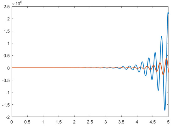
Figure 2. The state trajectories of open-loop systems with initial conditions (−2, 2).

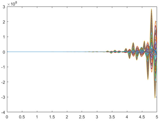
Figure 3. The state trajectories of open-loop systems with 100 different initial conditions ($x_1\in [-200,200]$, $x_2\in [-200,200]$).

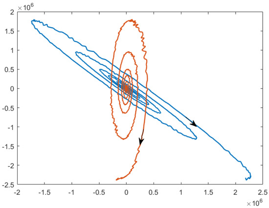
Figure 4. Phase plane of open-loop systems with initial conditions (−2, 2).

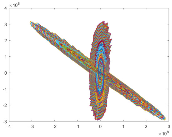
Figure 5. Phase plane of open-loop systems with 100 different initial conditions ($x_1\in [-200,200]$, $x_2\in [-200,200]$).

To finite-time stochastic stabilize the stochastic energy-storing circuit with time delay, the controller in the form of (30) has to be presented. Therefore, from the algorithm in Remark 4, the feasible solutions for LMI (31) are obtained as follows:

$$\begin{array}{c}\tilde{Q}=\left(\begin{array}{cc}42.2812& 1.1008\\ 1.1008& 138.2664\end{array}\right),\hfill \\ X=\left(\begin{array}{cc}45.6888& 0.9860\\ 0.9860& 2.5598\end{array}\right),\hfill \\ Y=\left(\begin{array}{cc}3.3174& -0.0047\\ 0.0248& 0.0341\end{array}\right),\hfill \\ K=\left(\begin{array}{cc}73.2569& -30.0688\\ 0.2573& 13.2114\end{array}\right),\hfill \\ {\epsilon }_1=41.8741,{\epsilon }_2=43.9821,{\epsilon }_3=1.9414,{\epsilon }_4=0.\hfill \end{array}$$

Correspondingly, choose the appropriate matrices $\overline{K}=\widehat{K}=diag(1,0.5)$. Obviously, $K_1^T{K}_1>0$ and $K_2^T{K}_2>0$ are satisfied. Then, the upper boundary of stochastic settling time function can be estimated in terms of (34)

$$E\left\{T_0(x_0,\omega )\right\}\le 6.4836.$$

(35)

Taking different initial conditions, the state trajectories of the closed-loop systems always converge to zero when $t\ge E\left\{T_0(x_0,\omega )\right\}=6.4836,$ which can be figured out in Figure 6 and Figure 7. That is to say, the stochastic energy-storing circuit with time delay is stochastic finite-time stable in terms of Definition 3, which also can be proved using the phase planes of Figure 8 and Figure 9.

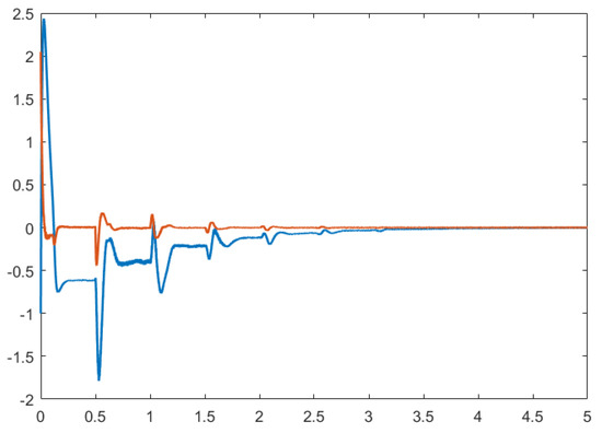
Figure 6. The state trajectories of closed-loop systems with initial conditions (−2, 2).

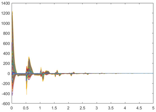
Figure 7. The state trajectories of closed-loop systems with 100 different initial conditions ($x_1\in [-200,200]$, $x_2\in [-200,200]$).

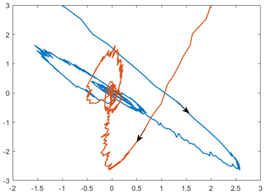
Figure 8. Phase plane of closed-loop systems with initial conditions (−2, 2).

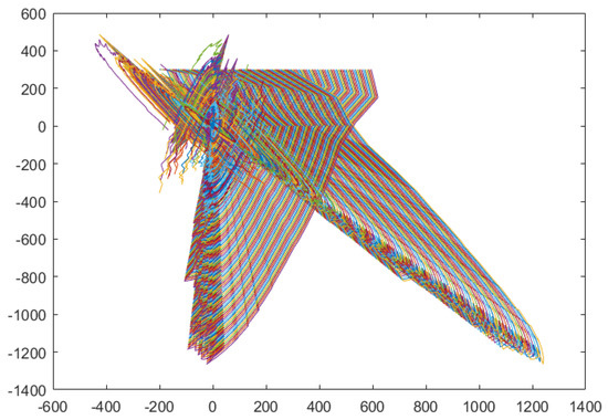
Figure 9. Phase plane of closed-loop systems with 100 different initial conditions ($x_1\in [-200,200]$, $x_2\in [-200,200]$).

If the time-delay term of the controller (30) is removed, that is $u\left(t\right)=-Kx\left(t\right)-\overline{K}{\left|x\left(t\right)\right|}^{\alpha }sgn\left(x\left(t\right)\right)$, the state trajectories of the stochastic energy-storing circuit with time delay are impossible to converge to zero when $t\ge E\left\{T_0(x_0,\omega )\right\}=6.4836,$ which is shown in Figure 10. Hence, our given results are correct and the proposed controller is effective.

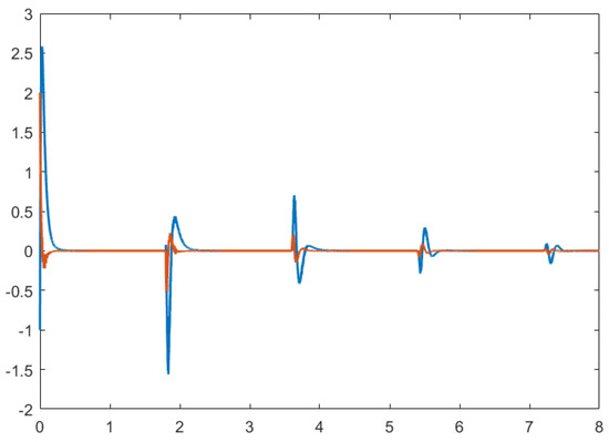
Figure 10. The state trajectories of closed-loop systems without the time-delay term of the controller.

5. Conclusions

In this paper, the finite-time stabilization problems for stochastic interval systems with time delay were investigated. The Lyapunov–Krasovskii functional and the $It\widehat{o}$’s formula were employed to derive some sufficient conditions such that the closed-loop system associated with a nonlinear state feedback controller was finite-time stochastic stable, which is different from the existing finite-time stochastic boundedness. The proposed control method was also applied to an energy-storing electrical circuit, in which not only the error of electronic components, but also the stochastic disturbance were considered. Various simulations have shown that the obtained results are correct and the proposed controllers are effective. In future work, we will focus on extending the proposed method to offshore platforms [44] and repetitive control systems [45,46].

References

- Park, M.J.; Kwon, O.M.; Ryu, J.H. Generalized integral inequality: Application to time-delay systems. Appl. Math. Lett. 2017, 77, 6–12. [Google Scholar] [CrossRef]
- Park, M.J.; Lee, S.H.; Kwon, O.M.; Ryu, J.H. Enhanced stability criteria of neural networks with time-varying delays via a generalized free-weighting matrix integral inequality. J. Frankl. Inst. 2018, 355, 6531–6548. [Google Scholar] [CrossRef]
- Zhang, X.-M.; Han, Q.-L.; Seuret, A.; Gouaisbaut, F.; He, Y. Overview of recent advances in stability of linear systems with time-varying delays. IET Control Theory Appl. 2019, 13, 1–16. [Google Scholar] [CrossRef]
- Xiao, S.-P.; Lian, H.; Teo, K.; Zeng, H.-B.; Zhang, X.-H. A new Lyapunov functional approach to sampled-data synchronization control for delayed neural networks. J. Frankl. Inst. 2018, 355, 8857–8873. [Google Scholar] [CrossRef]
- Zhang, B.-L.; Han, Q.-L.; Zhang, X.-M.; Yu, X. Sliding mode control with mixed current and delayed states for offshore steel jacket platform. IEEE Trans. Control Syst. Technol. 2014, 22, 1769–1783. [Google Scholar] [CrossRef]
- Park, M.J.; Kwon, O.M.; Ryu, J.H. Passivity and stability analysis of neural networks with time-varying delays via extended free-weighting matrices integral inequality. Neural Netw. 2018, 106, 67–78. [Google Scholar] [CrossRef]
- Zhang, X.-M.; Han, Q.-L. Abel lemma-based finite-sum inequality and its application to stability analysis for linear discrete time-delay system. Automatica 2015, 57, 199–202. [Google Scholar] [CrossRef]
- Yan, Y.; Huang, J. Cooperative output regulation of discrete-time linear time-delay multi-agent systems under switching network. Neurocomputing 2017, 241, 108–114. [Google Scholar] [CrossRef]
- Xiao, S.-P.; Xu, L.; Zeng, H.; Teo, K. Improved stability criteria for discrete-time delay systems via novel summation inequalities. Int. J. Control Automat. Syst. 2018, 16, 1592–1602. [Google Scholar] [CrossRef]
- Liu, Z.G.; Wu, Y.Q. Universal strategies to explicit adaptive control of nonlinear time-delay systems with different structures. Automatica 2018, 89, 151–159. [Google Scholar] [CrossRef]
- Zhang, X.-M.; Han, Q.-L.; Zeng, Z. Hierarchical type stability criteria for delayed neural networks via canonical Bessel-Legendre inequalities. IEEE Trans. Cybern. 2018, 48, 1660–1671. [Google Scholar] [CrossRef] [PubMed]
- Mahmoud, M.S.; Shi, P.; Shi, Y. Output feedback stabilization and disturbance attenuation of time-delay jumping systems. IMA J. Math. Control I 2018, 20, 179–199. [Google Scholar] [CrossRef]
- Wang, L.; Lam, H.K. A New Approach to Stability and Stabilization Analysis for Continuous-Time Takagi-Sugeno Fuzzy Systems With Time Delay. IEEE Trans. Fuzzy Syst. 2018, 26, 2460–2465. [Google Scholar] [CrossRef]
- Dong, C.; Gao, Q.; Xiao, Q.; Yu, X.; Pekař, L.; Jia, H. Time-delay stability switching boundary determination for DC microgrid clusters with the distributed control framework. Appl. Energy 2018, 228, 189–204. [Google Scholar] [CrossRef]
- Zhang, X.-M.; Han, Q.-L.; Wang, J. Admissible delay upper bounds for global asymptotic stability of neural networks with time-varying delays. IEEE Trans. Neural Netw. Learn. Syst. 2018, 29, 5319–5329. [Google Scholar] [CrossRef] [PubMed]
- Chen, G.C.; Gao, Y.; Zhu, S.S. Robust delay-feedback control for discrete-time stochastic interval systems with time-delay and Markovian jumps. In Proceedings of the 2017 Ninth International Conference on Advanced Computational Intelligence, Doha, Qatar, 4–6 February 2017; pp. 54–59. [Google Scholar]
- Chen, G.C.; Gao, Y.; Zhu, S.S. Finite-Time Dissipative Control for Stochastic Interval Systems with Time-Delay and Markovian Switching. Appl. Math. Comput. 2017, 310, 169–181. [Google Scholar]
- Zhu, S.; Shen, M.; Lim, C. Robust input-to-state stability of neural networks with Markovian switching in presence of random disturbances or time delays. Neurocomputing 2017, 249, 245–252. [Google Scholar] [CrossRef]
- Zhang, X.-M.; Han, Q.-L. Global asymptotic stability analysis for delayed neural networks using a matrix quadratic convex approach. Neural Netw. 2014, 54, 57–69. [Google Scholar] [CrossRef]
- Wang, B.; Zhu, Q. Stability analysis of semi-Markov switched stochastic systems. Automatica 2018, 94, 72–80. [Google Scholar] [CrossRef]
- Wang, J.; Zhang, X.-M.; Han, Q.-L. Event-triggered generalized dissipativity filtering for neural networks with time-varying delays. IEEE Trans. Neural Netw. Learn. Syst. 2016, 27, 77–88. [Google Scholar] [CrossRef]
- Lee, S.H.; Park, M.J.; Kwon, O.M. Synchronization criteria for delayed Lur’e systems and randomly occurring sampled-data controller gain. Commun. Nonlinear Sci. Numer. Simul. 2019, 68, 203–219. [Google Scholar] [CrossRef]
- Shen, M.; Ye, D. A finite frequency approach to control of Markov jump linear systems with incomplete transition probabilities. Appl. Math. Comput. 2017, 295, 53–64. [Google Scholar] [CrossRef]
- Chen, H.; Kang, W.; Zhong, S. A new global robust stability condition for uncertain neural networks with discrete and distributed delays. Int. J. Mach. Learn. Cybern. 2018, 142, 267–274. [Google Scholar] [CrossRef]
- Daniel, S.; Brad, P. Lyapunov stability theory of nonsmooth systems. IEEE Trans. Automat. Control 2018, 1, 416–421. [Google Scholar]
- Bhat, S.P.; Bernstein, D.S. Finite-Time Stability of Continuous Autonomous Systems. SIAM J. Control Optim. 2000, 38, 751–766. [Google Scholar] [CrossRef]
- Lin, X.; Zheng, Y. Finite-Time Consensus of Switched Multiagent Systems. IEEE Trans. Syst. Man Cybern. B 2017, 47, 1535–1545. [Google Scholar] [CrossRef]
- Chen, G.; Yang, Y. New necessary and sufficient conditions for finite-time stability of impulsive switched linear time-varying systems. IET Control Theory A 2018, 12, 140–148. [Google Scholar] [CrossRef]
- Guo, Z.; Gong, S.; Huang, T. Finite-time synchronization of inertial memristive neural networks with time delay via delay-dependent control. Neurocomputing 2018, 293, 100–107. [Google Scholar] [CrossRef]
- Liu, Y.; Ma, Y.; Wang, Y. Reliable finite-time sliding-mode control for singular time-delay system with sensor faults and randomly occurring nonlinearities. Appl. Math. Comput. 2018, 320, 341–357. [Google Scholar] [CrossRef]
- Zhang, L.; Qi, W.; Kao, Y.; Gao, X.; Zhao, L. New results on finite-time stabilization for stochastic systems with time-varying delay. Int. J. Control Automat. 2018, 16, 649–658. [Google Scholar] [CrossRef]
- Yang, X.; Li, X.; Jinde, C. Robust finite-time stability of singular nonlinear systems with interval time-varying delay. J. Frakl. Inst. 2018, 355, 1241–1258. [Google Scholar] [CrossRef]
- Liu, M.; Wu, H. Stochastic finite-time synchronization for discontinuous semi-Markovian switching neural networks with time delays and noise disturbance. Neurocomputing 2018, 310, 246–264. [Google Scholar] [CrossRef]
- Huang, X.; Ma, Y. Finite-time H∞, sampled-data synchronization for Markovian jump complex networks with time-varying delays. Neurocomputing 2018, 296, 82–99. [Google Scholar] [CrossRef]
- Li, S.; Peng, X.; Tang, Y.; Shi, Y. Finite-Time Synchronization of Time-Delayed Neural Networks with Unknown Parameters via Adaptive Control. Neurocomputing 2018, 308, 65–74. [Google Scholar] [CrossRef]
- He, S.P.; Liu, F. Stochastic finite-time control for uncertain jump system with energy-storing electrical circuit simulation. Int. J. Energy Environ. 2010, 1, 883–896. [Google Scholar]
- Vargas, A.N.; Pujol, G.; Acho, L. Stability of markov jump systems with quadratic terms and its application to rlc circuits. J. Frankl. Inst. 2016, 354, 332–344. [Google Scholar] [CrossRef]
- Odabasioglu, A.; Celik, M.; Pileggi, L.T. Practical Considerations For Passive Reduction of RLC Circuits. In Proceedings of the IEEE/ACM International Conference on Computer-Aided Design, San Jose, CA, USA, 7–11 November 1999; pp. 214–219. [Google Scholar]
- Turki, A.Q.; Mailah, N.F.; Othman, M.L.; Mohammad, L.; Sabry, A.H. Transmission lines modeling based on vector fitting algorithm and rlc active/passive filter design. Int. J. Simul. Syst. Sci. Technol. 2017, 17, 42.1–42.6. [Google Scholar]
- Chen, W.; Jiao, L.C. Finite-time stability theorem of stochastic nonlinear systems. Automatica 2010, 46, 2105–2108. [Google Scholar] [CrossRef]
- Yin, J.; Khoo, S.; Man, Z.; Yu, X. Finite-time stability and instability of stochastic nonlinear systems. Automatica 2011, 47, 2671–2677. [Google Scholar] [CrossRef]
- Wu, M.; He, Y.; She, J.H. Stability Analysis and Robust Control of Time-Delay Systems; Springer: Berlin, Germay, 2010; pp. 36–37. [Google Scholar]
- Mao, X. Stochastic Differential Equations and Applications, 2nd ed.; Horwood Publishing: Chichester, UK, 2007. [Google Scholar]
- Zhang, B.-L.; Han, Q.-L.; Zhang, X.-M. Recent advances in vibration control of offshore platforms. Nonlinear Dyn. 2017, 89, 755–771. [Google Scholar] [CrossRef]
- Zhou, L.; She, J.; Zhou, S.; Li, C. Compensation for state-dependent nonlinearity in a modified repetitive-control system. Int. J. Robust Nonlinear Control 2018, 28, 213–226. [Google Scholar] [CrossRef]
- Zhou, L.; She, J.; Zhou, S. Robust H∞ control of an observer-based repetitive-control system. J. Frankl. Inst. 2018, 355, 4952–4969. [Google Scholar] [CrossRef]
© 2019 by the authors. Licensee MDPI, Basel, Switzerland. This article is an open access article distributed under the terms and conditions of the Creative Commons Attribution (CC BY) license (http://creativecommons.org/licenses/by/4.0/).