Abstract
Conventional differential synthetic aperture radar tomography (D-TomoSAR) can only capture the scatterers’ one-dimensional (1-D) deformation information along the line of sight (LOS) of the synthetic aperture radar (SAR), which means that it cannot retrieve the three-dimensional (3-D) movements of the ground surface. To retrieve the 3-D deformation displacements, several methods have been proposed; the performance is limited due to the insufficient sensitivity for retrieving the North-South motion component. In this paper, an improved D-TomoSAR model is established by introducing the scatterers’ 3-D deformation parameters in slant range, azimuth, and elevation directions into the traditional D-TomoSAR model. The improved D-TomoSAR can be regarded as a multi-component two-dimensional (2-D) polynomial phase signal (PPS). Then, an effective algorithm is proposed to retrieve the 3-D deformation parameters of the ground surface by the 2-D product high-order ambiguity function (PHAF) with the relax (RELAX) algorithm. The estimation performance is investigated and compared with the traditional algorithm. Simulations and experimental results with semi-real data verify the effectiveness of the proposed signal model and algorithm.
1. Introduction
Differential synthetic aperture radar (SAR) tomography (D-TomoSAR) [1,2] is a kind of multi-baseline SAR processing framework that allows the joint resolution capability of multiple scatterers’ velocities and elevations in the same range-azimuth cell through a two-dimensional (2-D) baseline-time spectral estimation. It is favored over similar differential SAR interferometry (D-InSAR) technologies [3], such as persistent scatterer interferometry (PSI) [4,5] and small baseline subset (SBAS) [6], because D-TomoSAR can overcome the layover phenomenon in the forest or urban areas. At present, D-TomoSAR is widely used in mapping and monitoring the infrastructure deformation and ground subsidence caused by the over-pumping of groundwater or mining.
One of the disadvantages of the D-TomoSAR technique is that only one-dimensional (1-D) deformation along the radar line of sight (LOS) can be captured, which cannot fully describe the actual deformation information of ground. The extraction of three-dimensional (3-D) (East-West, North-South, Up-Down) deformation information plays an important role in monitoring seismic and volcanic activities and the urban surface subsidence. Thus, it is significant to decompose the observed 1-D LOS deformation information into the 3-D deformation parameters.
Several methods of 3-D deformation retrieval based on D-InSAR and D-TomoSAR technology have already been reported. These methods use a combination of multiple LOS deformation observations to retrieve the three deformation components [7,8], while the equal-precision 3-D deformation estimation cannot be obtained. In particular, the estimation error in the North-South direction is much greater than that in the other two directions. This is heightened by the fact that most of the spaceborne SARs in orbit fly along the near-pole orbits [8], namely, the azimuth direction of SAR imaging is almost parallel to the North-South direction. To improve the accuracy of North-South deformation retrieval from LOS measurements, several methods have been proposed, such as a combination of ascending/descending SAR acquisitions and the multi-aperture interferometry (MAI) algorithm [9] or offset-tracking [10] technology. However, these methods are only suitable for retrieving the large deformation caused by earthquakes or volcanic activities and are unable to be applied in D-TomoSAR directly because they are developed from D-InSAR. Combining the D-InSAR with global positioning system (GPS) data [11] is another approach to retrieving the 3-D deformation maps. Nevertheless, this method strongly depends on the external GPS data and cannot be widely used.
Results of existing methods for retrieving the 3-D deformation show that the higher the diversity of the geometric configuration (the satellite heading angle and incidence angle of antenna) of the combined SAR data is, the more accurate the North-South retrieval results will be [12]. This provides an effective way to improve the accuracy of North-South deformation retrieval. A common method is to combine the SAR data acquired from different incidence angles, e.g., combining SAR data acquired from the ascending and descending tracks with right- and left-looking configurations [13]. However, extreme attitude control is required for this method to change the incidence angle of the antenna, which is difficult for satellites with large antennas. Another method is to change the heading angle of the satellite and make it deviate from the North-South direction, which can fundamentally solve the problem of low precision of deformation estimation in the north component [14,15], whereas the satellite heading angle is directly related to the orbital inclination of the satellite, and the non-polar orbit will limit the imaging coverage in the latitudinal direction.
At present, the SuperSAR [12,16] and BiDiSAR [17] are proposed to improve the accuracy of the deformation retrieval in the North-South direction by increasing the squint angle of SAR imaging in D-InSAR. In this paper, an improved D-TomoSAR signal model is proposed by introducing the squint angle of SAR imaging into the traditional D-TomoSAR model to achieve a higher accuracy for North-South deformation estimation. In the proposed model, the relationship between the phase term of the improved D-TomoSAR and the 3-D deformation velocities in the slant range, azimuth, and elevation directions are established through imaging geometry. As a result, the elevation and 3-D deformation parameters of scatterers can be retrieved by estimating the coefficients of a 2-D polynomial phase signal (PPS). Analyses of numerical simulations and the semi-real data experiments indicate that a comparable effect to change the satellite heading angle can be achieved by increasing the squint angle of SAR imaging.
This paper is organized as follows. The improved D-TomoSAR signal model is proposed in Section 2. In Section 3, the 2-D product high-order ambiguity function (PHAF) with the relax (RELAX) algorithm is adopted to estimate the 3-D deformation components, and an analysis is carried out to evaluate the performance of the proposed model. Section 4 presents experiments on simulated and semi-real data to demonstrate the precision and efficiency of the proposed algorithm. A general conclusion is presented in Section 5.
2. System Model
2.1. Review of D-TomoSAR
The observation geometry of conventional D-TomoSAR is shown in Figure 1, where X represents the ground-range direction, Y is the azimuth direction, Z is the vertical height direction, r is the reference slant range direction along the LOS of the radar, and is the elevation direction orthogonal to the slant range-azimuth plane. Consider the processing of SAR acquisitions from N passes with M single looking complex (SLC) SAR images acquired simultaneously at each pass by M similar spaceborne SAR. Let , be the acquisition time of the phase centers in the nth pass, and let , be the imaging time of the mth SAR radar at the nth pass, thus, we have . The registration of the M × N SAR images to a reference master image is firstly performed, and the correction of atmospheric disturbance is carried out to eliminate the measurement noise in the SAR images. The focused complex-valued measurement of each calibrated range-azimuth pixels in the M × N SAR images can be arranged in the M × N baseline-time plane to form a data matrix G. Each element in this data matrix denotes the focused measurement of the range-azimuth pixel in SAR images acquired from the mth SAR radar at time , and it is the integral of the focused signal of scatterers distributed along the elevation direction s. As a result, can be written as:
where is the superposition of the backscattering function along elevation s in the pixel , is the wavelength, represents the distance between the scatterer located at coordinates of on the ground and the mth satellite at time , is the scatterers’ displacement in the LOS direction, is the 2-D point spread function (PSF) of the focused SAR image.
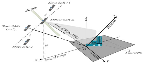
Figure 1.
System geometry of differential synthetic aperture radar tomography (D-TomoSAR).
For simplicity, we assume the 2-D PSF to approximate an ideal 2-D Dirac function, and a deramping operation [18] is performed to compensate the phase quadratic distortion of the received data. Finally, the focused measurement of each pixel , can be rewritten as:
Note that only the LOS deformation can be observed by the conventional D-TomoSAR system, and at least three LOS observations from different acquisition geometries are required to decompose the LOS displacement into the 3-D deformation components [8]. However, the deformation component in the North-South direction cannot be reliably resolved because the current SAR satellites operate in the near-polar orbits. To improve the accuracy of the North-South deformation retrieval, the usage of squint imaging mode is helpful, which was verified in the D-InSAR [12,16]. In this context, an improved D-TomoSAR signal model is proposed by introducing the 3-D deformation components of scatterers into the traditional D-TomoSAR system through the SAR squint imaging mode in this paper to achieve an improvement for the accuracy of deformation retrieval in the North-South direction.
2.2. Signal Model of Improved D-TomoSAR
As shown in Figure 2, P1 and Pm are the antenna phase center of the first and mth radar, respectively, and the corresponding imaging time for the same region is and . In this paper, the acquisition acquired from radar P1 at time is defined as the master image in the registration operation. The green plane is the 2-D imaging plane of the radar P1, and the point is the position of projecting the radar Pm onto the imaging plane of radar P1. B is the spatial baseline between P1 and Pm. is the horizontal baseline along the slant range direction, is the horizontal baseline along the azimuth direction, and is the orthogonal baseline along the elevation direction. The incidence angle of the beam center of P1 is α, and denotes the squint angle. is the distance between P1 at time and the reference point T0, whose elevation is zero. Accordingly, is the distance between Pm and the scatterer with an elevation s at time . is the reference range for the deramping operation, and it can be expressed as the distance between Pm and the reference point . The scatterer is assumed to occur in a 3-D displacement during the imaging time from to , where the deformation components in the slant range, azimuth, and elevation direction are , , and , respectively.
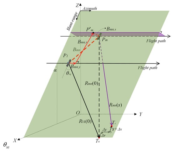
Figure 2.
Squinted synthetic aperture radar (SAR) data acquisition geometry for the improved D-TomoSAR.
Referring to Figure 2, and the reference range for the deramping operation can be expressed as:
As mentioned in (2), is given by:
where represents the inner product of the vectors. According to the Fresnel approximation, the difference in slant range can be rewritten as:
In this paper, we assume that the acquisitions were registered to the master image with subpixel accuracy. Hence, the horizontal baseline along the azimuth direction is nearly zero. In addition, the acquisitions acquired from different orbits were also corrected to the reference image with a constant slant range distance to eliminate the effect of the spatial decorrelation [19], by which the horizontal baseline along the slant range direction is also approximately equal to zero. On the other hand, the first term in (5) is a constant and will not affect the amplitude of the image [20]. As a result, the first term in (5) can be incorporated in the backscattering function . Finally, the focused measurement in the improved D-TomoSAR model can be expressed as:
where . Assuming that the 3-D deformation model of the scatterer follows the linear model, we have:
where , , and are the deformation velocities of the scatterer along the slant range, azimuth, and elevation directions, respectively. Finally, (6) can be rewritten as:
where is the elevation extent of the scatterers, and , , and are the range of possible velocities along the slant range, azimuth, and elevation, respectively.
In the conventional D-TomoSAR, the scatterers in each range-azimuth resolution cell are assumed to have only the linear displacement along the LOS direction, and the elevation and deformation parameters of the scatterers are independent of each other. As a result, the retrieval of the elevation and deformation parameters of scatterers fits well into the framework of 2-D spectral estimation. However, the elevation of each scatterer is coupled with its deformation parameter in the elevation direction in the improved D-TomoSAR signal model, as shown in (8). This means that the 2-D spectral estimation cannot be used to estimate the elevation and the 3-D deformation parameters for the improved D-TomoSAR.
In addition, no more than four scatterers are assumed to locate in the same range-azimuth resolution cell in most of the typical ground scenes [21]. Therefore, the backscattering coefficient in (8) can be assumed to be sparse in the object domain. Let K be the number of the scatterers lying in the same range-azimuth resolution cell, and the backscattering coefficient can be written as [22]:
where , , , and are the elevation and 3-D deformation components of the kth scatterer, respectively. The coefficient represents the complex amplitude of the kth scatterer. We assume that the PSF of the scatterers in the elevation and 3-D deformation direction is the ideal Dirac function in this paper. Substituting (9) into (8), we yield:
where is the residual error signal after atmospheric phase compensation. Inspecting the phase terms in (10), the improved D-TomoSAR model is found to be the multi-component second order 2-D PPS.
Let be a general discrete-time multi-component second order 2-D PPS, which can be expressed as:
where:
where and , K is the number of the components, and is the amplitude of the kth component. Comparing (10) with (11) and (12), we have:
Equation (13) reveals that the elevation and deformation parameters of scatterers can be retrieved by estimating the coefficients of the 2-D PPS shown in (11). Given that contains two unknowns— and —at least two sets of combined SAR acquisitions with different squint angles are required to solve the three deformation components of scatterers. In addition, the larger the diversity of the squint angles of the different combined acquisitions is, the higher the achieved precision would be for the 3-D retrieval [12].
3. 3-D Deformation Retrieval for the Improved D-TomoSAR
As can be seen from the previous section, the improved D-TomoSAR signal model can be equivalent to a multi-component 2-D PPS, and its coefficients correspond to the elevation and deformation parameters of the scatterers. However, different from the general 2-D PPS with uniform sampling, the equivalent 2-D PPS is typically non-uniform and very sparse in the spatial and temporal baseline plane. This is because the acquisitions from the D-TomoSAR system are obtained by a multiple-pass of SAR systems with nonuniformly spaced orbits, and only a limited number of SARs or channels are used to acquire the data for each pass. As a result, the traditional estimation algorithm for general 2-D PPS is unable to be applied to the improved D-TomoSAR directly.
Considering the above-mentioned, the 2-D product high-order ambiguity function (2-D PHAF) with the RELAX algorithm were proposed to achieve the estimations of the components in the 2-D PPS under the nonuniform and sparse sampled conditions [23]. In this section, the 2-D PHAF with the RELAX algorithm is firstly used to acquire the estimation of the coefficients in (10). Then, two sets of combined SAR acquisitions with different squint angles are adopted to retrieve the 3-D deformation velocities.
3.1. Review of the 2-D PHAF with RELAX Algorithm
For each single component in (11), its 2-D high-order instantaneous moment (HIM) of second order is defined in [24]:
where and are the lags. Then, the 2-D high-order ambiguity function (HAF) is defined as the 2-D Fourier transform of the 2-D HIM, thus, the 2-D HAF of is:
As mentioned in [24], the second order 2-D HIM of has a linear phase for a second order 2-D PPS. Thus, the phase coefficients of the single component 2-D PPS can be estimated by searching the location of the peak of the 2-D HAF. According to (11), (12), (14), and (15), the peak’s coordinates of the 2-D HAF of can be given by:
Inspecting (16), it is an equations group with two measurements— and —and three unknowns—, , and . Thus, at least two sets of lags are required to estimate these unknown parameters. Once the second order coefficients are estimated, the second order phase term in can be removed by a conjugate multiplication. After that, the original 2-D PPS degenerates into a one-order 2-D PPS whose phase coefficients can be achieved by the 2-D Fourier transform.
However, the pervious procedure is only applicable for the single component 2-D PPS. For the multi-component 2-D PPS, the cross terms caused by computing the 2-D HIM significantly affect the estimation results. In this case, the 2-D PHAF can be used to enhance the peaks of the auto terms and weaken the cross terms by multiplying the 2-D HAF with different sets of lags. Choosing L sets of the two lags as or , where , the second order 2-D PHAF with two lags can be given by:
where and are the two sets of lags vectors. and are the scaling factors to align the peaks of the auto terms. Let and , be the locations of the peaks of and , respectively. The second order phase coefficients of each component in (11) can be estimated as follows:
After estimating the second order coefficients of the kth component, we multiply the phase factor by the original signal in (11), then the kth component becomes a 2-D PPS of order one while the other components remain 2-D PPS of order two. Therefore, the 2-D Fourier transform can be used to estimate the first order coefficients of the kth component. Repeat the above procedure to achieve the estimates of the phase coefficients of all components.
The key problem of the above algorithm is calculating the spectrum of the 2-D HIM for searching the locations of the peaks of 2-D PHAF. However, the operation of (15) requires the uniform sampling of the signals with a sampling rate that satisfies the Nyquist theorem, thus, the original 2-D PHAF algorithm is unable to be applied to the D-TomoSAR model directly. In this context, the RELAX algorithm [23] is preferred to solve the above problem, and it is able to achieve the peak’s location of 2-D PHAF in low signal noise ratio (SNR).
3.2. 3-D Deformation Motion Retrieval
Using the 2-D PHAF with the RELAX algorithm, the elevation and deformation parameters of multiple scatterers located in the same slant range-azimuth resolution cell can be estimated, and the deformation parameters are given from (13) as follows:
where:
For one set of combined acquisitions with a non-zero squint angle, we have one measurement and two unknowns and . To retrieve these two unknown deformation components, at least two sets of combined SAR data with different squint angles are required. However, it should be noted that the slant range and azimuth direction are related to the SAR imaging geometry defined by the satellite heading and antenna incidence angle. Thus, the master images used in the two sets of combined data must be acquired by the same imaging geometry. This can be achieved by correcting the imaging geometry of master images into a reference geometry parameter through the registration operation. Assuming that the squint angles used in the two sets of combined acquisitions are and , respectively, (19) can be rewritten in the matrix form as:
where , , and .
Once the scatterers’ 3-D deformation components along the slant range, azimuth, and elevation directions are estimated, the observed 3-D deformation components can be mapped to the original 3-D deformation parameters of , , and in North-South, East-West, and Up-Down directions. Assuming that the antenna incidence angle is and the satellite heading angle is , as shown in Figure 3, the explicit projection relationship between the observed 3-D deformation parameters and the original deformation components can be written as:
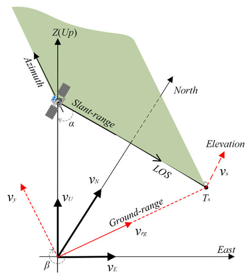
Figure 3.
Diagram for the original three dimensional (3-D) deformation components , , and in North-South, East-West, and Up-Down directions, and the displacement components , , and in ground-range, azimuth, and elevation directions.
Similarly, (22) can be rewritten in the matrix form as:
where , and .
Combining (21) with (23), we have:
Subsequently, the original 3-D deformation components in North-South, East-West, and Up-Down directions can be retrieved by weighted least squares as follows:
where is the covariance matrix caused by the residual atmospheric phase error of the measurements. Assuming the deformation parameters and acquired by the two sets of combined SAR data are independent, the non-diagonal elements in are zeros, and is only determined by its diagonal elements, i.e.,:
where are the estimation variance of the deformation parameters obtained by (19), respectively.
The results in (25) show that the accuracy of the 3-D deformation retrieval depends on the imaging geometry of the combined data. Here, we introduce the concept of position dilution of precision (PDOP) in the global navigation satellite system (GNSS) to assess the accuracy of the 3-D deformation retrieval [8,25]. According to the definition of PDOP, the estimation covariance matrix of 3-D deformation retrieval is:
The matrix is a square symmetric matrix, and its diagonal elements denote the estimation error variance for the 3-D deformation components. The smaller the value the diagonal element is, the higher the precision of the estimation result for the corresponding deformation component will be.
3.3. Performance of 3-D Deformation Estimation
In this sub-section, a comparison of 3-D deformation retrieval performance between the proposed algorithm in this paper and the traditional motion decomposition method in [8] is carried out. In [8], the 3-D deformation components are estimated by decomposing the multiple LOS displacement observed from different viewing geometries. As shown in Figure 3, the relation between LOS deformation measurement observed by the traditional D-TomoSAR and the 3-D displacement components can be written as:
The results in (28) show that at least three LOS measurements from different acquisition geometries are required to achieve the three deformation components , , and . Assuming is the deformation vector contains LOS observations, is the 3-D deformation vector consisting of the three deformation components in North-South, East-West, and Up-Down direction, and is the coefficient matrix corresponding to the projection vectors. As a result, the relationship between the multiple LOS measurements and the 3-D deformation components can be expressed as:
Accordingly, the estimation covariance matrix of 3-D deformation retrieval from (29) can be written as:
where represents the covariance matrix of the LOS measurements.
To analyze the performance of the proposed and the traditional methods objectively, three cases of geometric configurations of acquisitions were considered. For the first two cases, three stacks of combined data were adopted, and the acquisitions were all obtained from stripmap mode of SAR with a squint angle of zero. In Case I, the first two stacks were both acquired from the ascending orbit, while the third stack was acquired from the descending orbit. In Case II, we changed the satellite heading angle of the third stack to keep it away from the near-polar orbit to evaluate the effect of the heading angle for the 3-D deformation retrieval. Finally, the 3-D deformation parameters were retrieved by the traditional method from three LOS deformation measurements, as shown in (28). For comparisons, in Case III, we considered two stacks of combined data with different squint angles to retrieve the 3-D deformation parameters with the proposed method.
It should be noted that the estimation covariance matrix (27) and (30) are related to the measurement covariance matrix and , which are dependent on the SNR of acquisitions and the variance of the temporal baseline distribution. In order to evaluate the effect of variation of geometry for the 3-D deformation retrieval, we set the elements in the matrix and to be [8]. The geometric configurations of combined data are detailed in Table 1. Accordingly, the standard deviations of the estimation of 3-D deformation components in these three cases can be calculated by (27) and (30), respectively, as shown in Table 1.

Table 1.
Acquisition parameters of each scenarios and the performance of 3-D retrieval.
Results of Case I in Table 1 show that the accuracy of the deformation component in North-South direction was far lower than that of the other two directions due to the influence of the near-polar orbits. Therefore, the traditional 3-D deformation retrieval mode cannot reliably estimate the North-South motion parameter. Compared with Case I, the third set of data in Case II was acquired from the non-polar orbit. The experimental results show that the accuracy of the North-South deformation component could be improved by changing the satellite heading angle to make it deviate from the near-polar orbit. In Case III, two sets of combined data with different squint angles were adopted to retrieve the 3-D deformation components by using the proposed method. We can draw a conclusion that the existence of squint angles of combined data can improve the sensitivity to the North-South component retrieval and achieve a comparable effect as changing the satellite heading angle from the experimental results of Case III.
Although changing the satellite heading angle can improve the accuracy of the North-South deformation component, the satellite with non-polar orbit limits the latitudinal imaging coverage, as shown in the results of Cases II and III. On the contrary, the proposed method only uses the squint imaging mode of SAR with no changes to the existing satellite orbit design, which provides an effective way to enhance the North-South deformation component. To further verify the effectiveness of the proposed method, a detailed comparison analysis between Case II and Case III is presented. Firstly, we considered a scenario with three stacks of acquisitions. The geometric configurations of first two stacks were same as Case II, while the third stack had a varying satellite heading angle in the range of 187 degrees to 260 degrees. Figure 4a depicts the 3-D deformation precision as a function of the satellite heading angle. The results indicate that the accuracy of the North-South deformation component could be significantly improved by changing the heading angle of the satellite to make it deviate from the near-polar orbit. Secondly, we evaluated the effect of squinted acquisitions by using the geometric configurations in Case III, where the squint angle of first stack was fixed to 5 degrees, and another one changed from 6 degrees to 40 degrees. In this case, the 3-D deformation precisions are shown in Figure 4b. Comparing Figure 4a with Figure 4b, we find that a squint angle yields an effect comparable to changing the satellite heading angle.
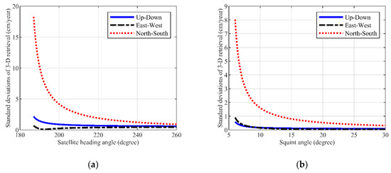
Figure 4.
Impact of changing the satellite heading angle and using the acquisitions with different squint angles for the 3-D deformation retrieval. (a) and (b) are the diagrams of the standard deviations of 3-D retrieval varying with the satellite heading angle and squint angle, respectively.
3.4. Some Considerations
3.4.1. Resolution Analysis
Here, the analysis of the resolution for the proposed algorithm is presented. According to [26], the resolution of the elevation estimation of a scatterer is determined by the overall orthogonal baseline length. Therefore, the Rayleigh resolution of the elevation estimation is:
where is the overall orthogonal baseline length.
Similarly, the resolution of the 3-D deformation velocity is determined by the span of time baseline, and the resolution of 3-D velocity along the slant range, azimuth, and elevation directions are expressed as follows:
where T is the span of time baseline.
It can be seen that the resolution of deformation velocity in slant range and azimuth directions are related to the squint angle of the SAR imaging.
3.4.2. Discussion about the Nonlinear Deformation
In (7), a linear deformation model of scatterers was assumed in this paper. However, in reality, the deformation can be nonlinear. Therefore, it is necessary to analyze the performance of the proposed algorithm in the nonlinear deformation case.
Generally, the most common types of nonlinear motion of scatterers are accelerating motion and periodic motion [27]. Among them, the accelerating motion may be caused by the over-exploitation of groundwater or minerals, while the thermal dilation effect of scatterers caused by the seasonal temperature variations usually presents as a periodic movement characteristic. Therefore, the following analyses are divided into two cases: (a) the deformation of the scatterer contains linear and accelerating motions; (b) the deformation of the scatterer contains linear and periodic motions. In addition, we also give a brief analysis of the mixed deformation, which contains both of the above kinds of motions.
(a) Deformation contains linear and accelerating motion:
In this case, the 3-D deformation model described in (7) can be rewritten as:
where , , and are the deformation accelerations of the scatterers along the slant range, azimuth, and elevation directions, respectively.
Substituting (33) into (6) and using the discretization operation, we have:
Similarly, inspecting the phase terms in (34), the signal model can be regarded as a multi-component fourth order 2-D PPS. Accordingly, the relationship between the phase coefficients in (34) and those of the general fourth order 2-D PPS can be expressed as:
Since the original 2-D PHAF algorithm is suitable for solving the high-order 2-D PPS, the phase coefficients in (34) can still be estimated by using the proposed algorithm in this paper. Once the estimations of phase coefficients in (34) are achieved, the elevation, 3-D deformation velocity and 3-D deformation acceleration of scatterer can be estimated from the following equations:
According to (36) and (37), at least two sets of SAR acquisition with different squint angles are required to solve the 3-D deformation velocities and accelerations of scatterers. However, it should be noted that in the process of phase coefficients estimation using the PHAF-based algorithm, the phase differentiation technique is employed to reduce the order of the PPS. Thus, the estimation errors of the highest-order coefficient affect the estimation of low-order coefficients, which is a so-called error propagation phenomena. As a result, it is necessary to improve the SNR of the SAR data to retrieve the 3-D deformation parameters of scatterers accurately.
(b) Deformation contains linear and periodic motion:
Previous research has shown that with the decrease of wavelength, SAR sensors are more sensitive to small surface displacements. Especially in urban areas, buildings with steel structures such as roofs, bridges, and tunnels not only have linear deformation displacement but are also affected by the nonlinear seasonal deformation caused by the thermal dilation effects [28].
Generally, there are two methods to retrieving the nonlinear seasonal deformation component. One is to use the temperature distribution of the monitoring area at the imaging time to form a synthetic aperture to carry out the five-dimensional (5-D) imaging. However, this method is not an optimal strategy because sometimes the temperature data of the monitoring area at the acquisition instants are difficult obtain, and the real temperature corresponding to the different structures also depends on the solar irradiation and the materials of the area. An alternative method is to use a sinusoidal function to simulate the thermal dilation effects caused by the seasonal temperature variations [27,29,30], which was proven to be effective under the condition of missing the temperature of the monitoring area. Therefore, in this part of the analysis, the periodic motion of the scatterer is described by a sinusoidal function rather than the former method. In this case, the 3-D deformation model described in (7) can be rewritten as:
where , , and are the amplitude of the periodic motion of the scatterers along the slant range, azimuth, and elevation directions, respectively. f is the seasonal frequency. It should be noted that the period of the seasonal temperature variations is one year, thus, .
Similarly, substituting (38) into (6) and using the discretization operation, we have:
The signal shown in (39) is a multi-component 2-D hybrid sinusoidal frequency modulated (FM) and PPS (2-D hybrid sinusoidal FM-PPS), while the algorithm proposed in this paper is only suitable for the pure 2-D PPS. Therefore, in this case, the amplitude of the periodic motion of the scatterer is unable to be estimated. Moreover, owing to the existence of the periodic motion of the scatterer, the estimation error of linear deformation is increased.
In conclusion, for the scatterer with linear and accelerating motion, the proposed algorithm can be used to estimate the 3-D velocity and 3-D acceleration of the deformation. However, in order to achieve the accurate estimation results, a high SNR of the SAR acquisitions is required. For the scatterer with linear and periodic motion, only the linear deformation components with large estimation errors can be obtained by using the proposed algorithm, and the amplitude of the periodic motion fails to be achieved. Furthermore, when the scatterer contains the above three kinds of deformation, the estimation errors of 3-D deformation velocities and 3-D accelerations are further increased.
4. 3-D Deformation Retrieval Simulation
In this section, simulation experiments are carried out to verify the effectiveness of the proposed model and algorithm. In the following experiments, two sets of combined acquisitions were acquired to retrieve the 3-D deformation by using the pursuit monostatic mode of a bistatic SAR system through repeat-passes [31]. In order to be more realistic, the system parameters of TanDEM-X are introduced here for the simulation of bistatic SAR system in this paper, and the system parameters for each SAR sensor are shown in Table 2. The experiments in this section were composed of two parts; the first part was the numerical simulation experiment for point targets, and the second one was the validation performance for the scene target using the semi-real data.
Table 2.
Simulation parameters of SAR systems for 3-D deformation retrieval.
4.1. Numerical Simulation for Point Target
In this part, the point targets simulation was performed to verify the effectiveness of the proposed improved D-TomoSAR model, and the accuracy of the 3-D deformation retrieval was analyzed. To this end, we assumed that there were a total of three scatterers located in a same slant range-azimuth resolution cell along the elevation direction. The scatterers’ elevations and the 3-D deformation velocities in East-West, North-South, and Up-Down directions are listed in Table 3. Accordingly, the corresponding scatterers’ 3-D deformation velocities in slant range, azimuth, and elevation directions under the case of squint imaging mode can be calculated, which is also listed in Table 3. The Gaussian random noise with a mean value of zero and a standard deviation of 1 cm/year was added to the 3-D deformation velocities of each scatterer for realistic purpose. Previous results show that the combined data for the 3-D deformation retrieval needed to be acquired by the 2-D imaging of SAR. However, due to the existence of the squint angle, the conventional focusing algorithm for the side-looking SAR could not be applied to the squint mode SAR imaging directly. At this point, the algorithm in [32] was adopted to achieve the 2-D SAR imaging. This algorithm could still provide a stable 2-D focusing performance with a squint angle of 65 degrees, which meets the requirement of the 2-D imaging with squint mode in this paper. To approach the real imaging environment, the signal received by the SAR system was added by Gaussian noise with SNR = 5 dB in this experiment.
Table 3.
Elevation and deformation parameters of scatterers.
To retrieve the 3-D deformation parameters of scatterers, two SAR sensors in Table 2 were used through 30 repeat-passes to achieve two stacks of combined SAR acquisitions with different squint angles. Subsequently, the scatterers’ elevation s and the deformation parameters and in (19) could be estimated by the 2-D PHAF with the RELAX algorithm for each combined SAR acquisition. The estimated results are shown in Figure 5a,b. Finally, the estimation of 3-D deformation components in the slant range, azimuth, and elevation directions could be obtained by using the weighted least squares method to solve (21), and the retrieved results are summarized in Table 4. The experimental results show that the estimations of the 3-D deformation in three directions were very close to the real values. The estimation error was less than 0.5 cm/year in the slant range and the elevation direction and was no more than 1 cm/year in the azimuth direction. Although the accuracy of deformation estimation in azimuth direction was inferior to the other two directions, the proposed method still achieved a great improvement in accuracy of retrieval for the azimuth direction deformation compared with the traditional method. This proves the effectiveness of the proposed improved D-TomoSAR model, which provides a feasible solution to the realization of estimations of the 3-D deformation. Furthermore, once the 3-D deformation components along the slant range, azimuth, and elevation direction were estimated, the corresponding deformation parameters in North-South, East-West, and Up-Down directions could be calculated by (25), as shown in Table 5.
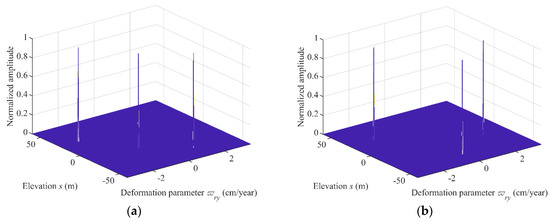
Figure 5.
Estimation of elevation and deformation parameters of two stacks of combined acquisitions. (a) The result of first stack with a squint angle of 5 degrees. (b) The result of second stack with a squint angle of 21.3 degrees.
Table 4.
Estimation of elevation and 3-D deformation velocity of three scatterers in slant range, azimuth, and elevation directions.
Table 5.
Estimation of elevation and 3-D deformation velocity of three scatterers in East-West, North-South, and Up-Down directions.
Furthermore, in order to illustrate the advantages of the proposed algorithm, the above estimation results were compared with the motion decomposition method [8]. In the following comparative simulation, three sets of SAR acquisitions were used to retrieve the 3-D deformation components. The parameters of SAR satellites shown in Table 1 of [8] were adopted for this experiment, as shown in Table 6.
Table 6.
Parameters of each satellite in [8].
First, three sets of SAR acquisitions for the D-TomoSAR processing were obtained by the three satellites in Table 6 through 30 repeat-passes. Then, the sparse reconstruction algorithm was used to estimate the LOS deformation velocities for each set of SAR acquisitions. As a result, three LOS deformation observations from different acquisition geometries were obtained, and the reconstructed elevations and deformation velocities for the three sets of SAR acquisitions are shown in Figure 6. The estimations of deformation velocity along LOS are listed in Table 7. Subsequently, the L1-norm minimization algorithm in [8] was used to decompose the LOS observations to achieve the 3-D deformation components, and the estimated results are summarized in Table 8.
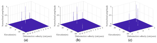
Figure 6.
Estimation of elevation and deformation parameters along line of sight (LOS). (a–c) correspond to the estimated results of Satellite 1, Satellite 2, and Satellite 3, respectively.
Table 7.
The results of the LOS deformation estimations.
Table 8.
Results of 3-D deformation estimations using the motion decomposition [8].
As can be seen from the comparison of Table 5 and Table 8, the flight directions of the satellites were almost parallel to the North-South direction owing to the SAR satellites operating in the near-polar orbit. Thus, the method of motion decomposition was insensitive to the North-South deformation retrieval, which led to a large estimation error. As mentioned by the authors of [8], precise unambiguous retrieval of the North-South component is not possible when only using the geometry configuration of current SAR satellites. The experimental results of the above simulation also draw the same conclusion. Therefore, the feasibility of the proposed algorithm in this paper for retrieving the 3-D deformation components was further verified by the analysis of the compared experiment.
According to Table 4, the estimation errors were not very small, especially for . Nevertheless, the accuracy of the estimation in the azimuth (North-South) direction also greatly improved compared with the motion decomposition method [8] shown in Table 8. In addition, compared with the decomposition method, the proposed algorithm only needed two sets of SAR acquisitions with different oblique angles without changing the orbit of the SAR satellite, which is conducive to practical application. On the other hand, as can be seen from Table 1 and Figure 4, the higher diversity of the squint angles between the two sets of SAR acquisitions, the more precise the deformation estimation in North-South was. In the above simulation, the estimated results of Table 4 were obtained by using the SAR acquisitions with squint angles of 5 degrees and 21.3 degrees, respectively. In order to further improve the accuracy of the deformation estimation in the azimuth direction, it is necessary to increase the diversity of the squint angles between the two sets of SAR acquisitions. To illustrate this point, an additional experiment was performed. The parameters used in this experiment were similar to those in Table 2, except that the squint angle of Satellite 2 increased from 21.3 degrees to 45 degrees. Then, the same simulation scenario was adopted, and the estimation results of the 3-D deformation in the slant range, azimuth, and elevation directions are shown in Table 9. The experimental results show that the accuracy of the deformation estimation in the azimuth direction improved with the increase in the diversity of the squint angles, which verifies the correctness of the above conclusions.
Table 9.
Estimation of 3-D deformation velocity of three scatterers in large diversity of squint angles between two sets of SAR acquisitions.
In addition, we set the variation of the SNR of SAR imaging in the range of [−10 dB, 15 dB] to evaluate the effect of noise on the elevation and the 3-D deformation retrieval. For each SNR, 250 simulations were performed. The parameters of scatterers are shown in Table 2. Figure 7 presents the three scatterers’ average estimation errors of elevation and 3-D deformation velocities as a function of the SAR imaging SNR, showing the performance improvement of the estimation when increasing the SNR of SAR imaging. For SNR = 5dB, the average error of elevation estimation was less than 0.4 m, and the error of deformation velocity estimations were no more than 0.5 cm/year in the slant range and elevation directions. The error of deformation estimation in the azimuth direction was larger than that in the other two directions due to the inadequate angular diversity of the squint angles used in the two combined acquisitions. Table 10 summarizes the elevation and 3-D deformation retrieval in the different SNRs. The experimental results show that the elevation and 3-D deformation velocities could be still estimated accurately and robustly by the proposed algorithm at a low SNR.
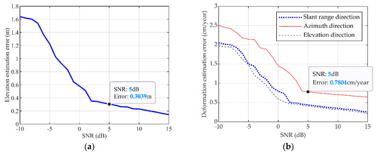
Figure 7.
Average estimation errors of elevation and 3-D deformation velocities. (a) Average estimation error of elevation. (b) Average estimation errors of 3-D deformation velocities in slant range, azimuth, and elevation directions.
Table 10.
Elevation and 3-D deformation retrieval errors in different signal noise ratios (SNRs).
4.2. Experiment with Semi-Real Data
In this part, an experiment was performed to verify the effectiveness of the proposed method for the scene target by using the semi-real data. In this experiment, we used Giorgio Franceschetti’s method [33] to generate the SAR raw data. The digital elevation model (DEM) data provided by Shuttle Radar Topography Mission (SRTM) were used as the terrain data, as shown in Figure 8a, and the deformation velocity maps in slant range, azimuth, and elevation directions were simulated in the corresponding scene, respectively, as shown in Figure 8b–d. The parameters of SAR systems are shown in Table 2.
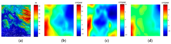
Figure 8.
The terrain and the simulation of the deformation maps: (a) digital elevation model (DEM) data from SRTM. (b–d) are the simulated deformation velocity maps in slant range, azimuth, and elevation direction, respectively.
Figure 9a illustrates one of the semi-real SAR images as an example. The elevation and deformation parameters are estimated by the proposed algorithm, and the results are as follows: Figure 9b is the estimation of elevation; Figure 9c–e are the estimations of deformation velocities in slant range, azimuth, and elevation directions, respectively. It can be seen that the estimated deformation in the three directions had the same trend as the real deformation map. The black line in Figure 9b shows the position of the analysis slice, and the estimation errors of 3-D deformation velocities for the scatterers located in this line are presented in Figure 10. Similar to the experimental results in the previous sub-section, the estimation errors in the slant range and elevation direction were also no more than 0.5 cm/year, and the accuracy of deformation retrieval in the azimuth direction was worse than that in the other two directions. Nevertheless, according to Figure 4b, the accuracy of the estimation in the azimuth direction could be improved by increasing the angular diversity of the squint angles used in the two combined acquisitions. Experimental results show the potential of the proposed algorithm for the reconstruction of the elevation and deformation parameters from the full SAR image.
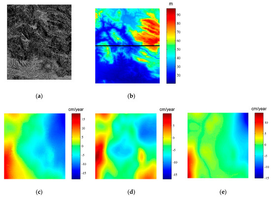
Figure 9.
Results of the estimations: (a) SAR simulated image generated by Giorgio Franceschetti’s method. (b) is the estimation result of elevation. (c–e) are the estimations of deformation velocity in the direction of slant range, azimuth, and elevation.
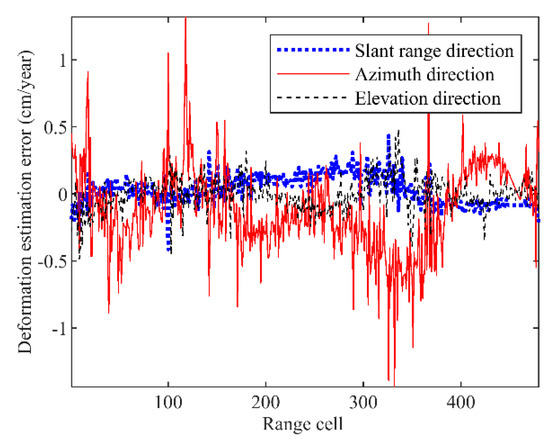
Figure 10.
The estimation errors of 3-D deformation velocities for the scatterers located in the slice.
In the above experiment with semi-real data, the DEM data were used to generate the SAR raw data in a natural scene, and the layover phenomenon was ignored. However, the D-TomoSAR was mainly applied to monitor the scenario with layover phenomenon such as urban areas and forests. Therefore, a semi-real SAR raw data of the urban area was simulated to further verify the effectiveness of the proposed algorithm. The DEM data of Shanghai was adopted to simulate the urban scene in this experiment, as shown in Figure 11. The red box in Figure 11 is the region of interest (ROI), which contains some buildings. Thus, the layover phenomenon occurs when imaging for the ROI. Assuming that each slant range-azimuth resolution cell of the SAR image in the ROI contains two scatterers, we call them the dominant scatterer and the secondary scatterer. Accordingly, the elevation and deformation maps of the ROI are simulated, shown as in Figure 12, where Figure 12a,e are the elevation of dominant scatterer and secondary scatterer, respectively. Figure 12b–d show the deformation velocities of the dominant scatterer along the slant range, azimuth, and elevation directions respectively, while Figure 12f–h correspond to the secondary scatterer.
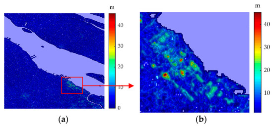
Figure 11.
DEM data of Shanghai, where the red box area is the region of interest (ROI). (a) DEM data, (b) DEM of the ROI.
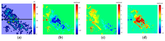
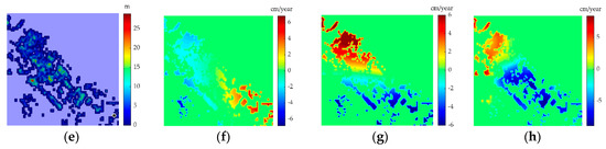
Figure 12.
The simulation of elevation and deformation maps. (a–d) are the simulated elevation of the dominant scatterer and its simulated deformation velocities along the slant range, azimuth, and elevation directions, respectively. (e–h) correspond to the secondary scatterer.
The proposed algorithm was used to estimate the elevation and the deformation velocity of the ROI, and the estimation results are shown in Figure 13. It can be seen from the experimental results that the estimated elevation and the 3-D deformation velocities of the dominant scatterer and secondary scatterer had the same trend as the true values. Similarly, the estimation errors of elevation and deformation velocity of scatterers located at the slice in Figure 12a were calculated, as shown in Figure 14. The experimental results show that the estimation results were consistent with our expectation, which validates the ability of the proposed algorithm to retrieve the elevation and 3-D deformation parameters in the scenario with layover phenomenon.
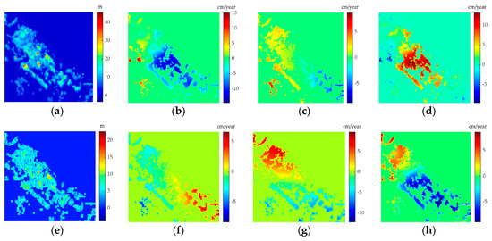
Figure 13.
Estimations of elevation and deformation maps. (a–d) are the estimated elevation of the dominant scatterer and its estimated deformation velocities along the slant range, azimuth, and elevation directions, respectively. (e–h) correspond to the secondary scatterer.
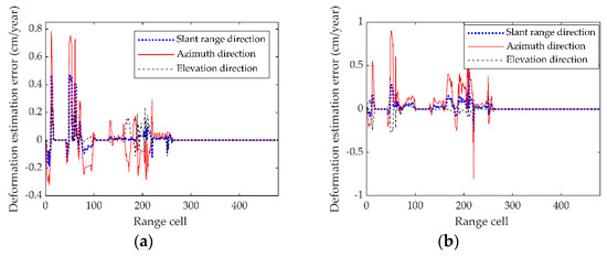
Figure 14.
The estimation errors of 3-D deformation velocities for the scatterers located in the slice of Figure 12a. (a) dominant scatterer. (b) secondary scatterer.
5. Conclusions
In this paper, a method is proposed for retrieving the elevation and 3-D deformation velocities of ground from an improved D-TomoSAR system model. Firstly, the relationship between the phase term of the improved D-TomoSAR and the 3-D deformation displacements is established from the imaging geometry of the D-TomoSAR system. The improved D-TomoSAR signal model can be regarded as a 2-D PPS, thus, the 2-D PHAF with the RELAX algorithm is introduced to estimate the elevation and 3-D deformation velocities of scatterers. Subsequently, the theoretical accuracy of 3-D deformation retrieval of the improved D-TomoSAR system is analyzed with respect to the squint angle of SAR imaging. In addition, the performance to assess the 3-D deformation retrieval of the proposed algorithm and the traditional method is compared. Results show that increasing the squint angle of SAR imaging and changing the satellite heading angel have a comparable effect on improving the accuracy of deformation retrieval in North-South direction. Finally, simulation and semi-real data results demonstrate the effectiveness and accuracy of the proposed method.
Author Contributions
Z.W. conceived and designed the method; M.L. guided the students to complete the research; Z.W. and K.L. performed the experiments and analyzed the performance; and Z.W. wrote the paper.
Funding
This research was funded by the National Natural Science Foundation of China, grant number 61771164 and the Innovation of Science and Technology Program of Shanghai Aerospace Science and Technology Corporation 2017.
Acknowledgments
The authors would like to thank the anonymous reviewers for their constructive comments and suggestions which are helpful in improving the readability of this paper.
Conflicts of Interest
The authors declare no conflict of interest.
References
- Lombardini, F. Differential tomography: A new framework for SAR interferometry. IEEE Trans. Geosci. Remote Sens. 2005, 43, 37–44. [Google Scholar] [CrossRef]
- Zhu, X.X.; Wang, Y.; Montazeri, S.; Ge, N. A Review of Ten-Year Advances of Multi-Baseline SAR Interferometry Using TerraSAR-X Data. Remote Sens. 2018, 10, 1374. [Google Scholar] [CrossRef]
- Drews, R.; Rack, W.; Wesche, C.; Helm, V. A spatially adjusted elevation model in Dronning Maud Land, Antarctica, based on differential SAR interferometry. IEEE Trans. Geosci. Remote Sens. 2009, 47, 2501–2509. [Google Scholar] [CrossRef]
- Ferretti, A.; Prati, C.; Rocca, F. Permanent scatterers in SAR interferometry. IEEE Trans. Geosci. Remote Sens. 2001, 39, 8–20. [Google Scholar] [CrossRef]
- Ferretti, A.; Fumagalli, A.; Novali, F.; Prati, C.; Rocca, F.; Rucci, A. A new algorithm for processing interferometric data-stacks: SqueeSAR. IEEE Trans. Geosci. Remote Sens. 2011, 49, 3460–3470. [Google Scholar] [CrossRef]
- Berardino, P.; Fornaro, G.; Lanari, R.; Sansosti, E. A new algorithm for surface deformation monitoring based on small baseline differential SAR interferograms. IEEE Trans. Geosci. Remote Sens. 2002, 40, 2375–2383. [Google Scholar] [CrossRef]
- Pepe, A.; Solaro, G.; Calo, F.; Dema, C. A minimum acceleration approach for the retrieval of multiplatform InSAR deformation time series. IEEE J. Sel. Top. Appl. Earth Obs. Remote Sens. 2016, 9, 3883–3898. [Google Scholar] [CrossRef]
- Montazeri, S.; Zhu, X.X.; Eineder, M.; Bamler, R. Three-dimensional deformation monitoring of urban infrastructure by tomographic SAR using multitrack TerraSAR-X data stacks. IEEE Trans. Geosci. Remote Sens. 2016, 54, 6868–6878. [Google Scholar] [CrossRef]
- Liang, C.; Fielding, E.J. Measuring azimuth deformation with L-band ALOS-2 ScanSAR interferometry. IEEE Trans. Geosci. Remote Sens. 2017, 55, 2725–2738. [Google Scholar] [CrossRef]
- Milillo, P.; Minchew, B.; Simons, M.; Agram, P.; Riel, B. Geodetic imaging of time-dependent three-component surface deformation: Application to tidal-timescale ice flow of Rutford ice stream, West Antarctica. IEEE Trans. Geosci. Remote Sens. 2017, 55, 5515–5524. [Google Scholar] [CrossRef]
- Razi, P.; Sumantyo, J.T.S.; Perissin, D.; Kuze, H.; Chua, M.Y.; Panggabean, G.F. 3D Land Mapping and Land Deformation Monitoring Using Persistent Scatterer Interferometry (PSI) ALOS PALSAR: Validated by Geodetic GPS and UAV. IEEE Access 2018, 6, 12395–12404. [Google Scholar] [CrossRef]
- Ansari, H.; De Zan, F.; Parizzi, A.; Eineder, M.; Goel, K.; Adam, N. Measuring 3-D surface motion with future SAR systems based on reflector antennae. IEEE Geosci. Remote Sens. Lett. 2016, 13, 272–276. [Google Scholar] [CrossRef]
- Rocca, F. 3D motion recovery with multi-angle and/or left right interferometry. In Proceedings of the Third International Workshop on ERS SAR, Frascati, Italy, 3–5 December 2003. [Google Scholar]
- Kou, L.; Wang, X.; Xiang, M.; Zhu, M. Interferometric estimation of three-dimensional surface deformation using geosynchronous circular SAR. IEEE Trans. Aerosp. Electron. Syst. 2012, 48, 1619–1635. [Google Scholar] [CrossRef]
- Liu, F.; Fan, X.; Zhang, T.; Liu, Q. GNSS-Based SAR Interferometry for 3-D Deformation Retrieval: Algorithms and Feasibility Study. IEEE Trans. Geosci. Remote Sens. 2018, 56, 5736–5748. [Google Scholar] [CrossRef]
- Jung, H.S.; Lu, Z.; Shepherd, A.; Wright, T. Simulation of the SuperSAR multi-azimuth synthetic aperture radar imaging system for precise measurement of three-dimensional Earth surface displacement. IEEE Trans. Geosci. Remote Sens. 2015, 53, 6196–6206. [Google Scholar] [CrossRef]
- Mittermayer, J.; Wollstadt, S.; Prats-Iraola, P.; López-Dekker, P.; Krieger, G.; Moreira, A. Bidirectional SAR Imaging Mode. IEEE Trans. Geosci. Remote Sens. 2013, 51, 601–614. [Google Scholar] [CrossRef]
- Fornaro, G.; Lombardini, F.; Serafino, F. Three-dimensional multipass SAR focusing: Experiments with long-term spaceborne data. IEEE Trans. Geosci. Remote Sens. 2005, 43, 702–714. [Google Scholar] [CrossRef]
- Reigber, A.; Moreira, A. First demonstration of airborne SAR tomography using multibaseline L-band data. IEEE Trans. Geosci. Remote Sens. 2000, 38, 2142–2152. [Google Scholar] [CrossRef]
- Fornaro, G.; Serafino, F.; Soldovieri, F. Three-dimensional focusing with multipass SAR data. IEEE Trans. Geosci. Remote Sens. 2003, 41, 507–517. [Google Scholar] [CrossRef]
- Zhu, X.X.; Bamler, R. Tomographic SAR inversion by L1-norm regularization-The compressive sensing approach. IEEE Trans. Geosci. Remote Sens. 2010, 48, 3839–3846. [Google Scholar] [CrossRef]
- Budillon, A.; Evangelista, A.; Schirinzi, G. Three-dimensional SAR focusing from multipass signals using compressive sampling. IEEE Trans. Geosci. Remote Sens. 2011, 49, 488–499. [Google Scholar] [CrossRef]
- Liu, M.; Wang, Z.; Wang, P. Extension of D-TomoSAR for multi-dimensional reconstruction based on polynomial phase signal. IET Radar Sonar Navig. 2018, 12, 449–457. [Google Scholar] [CrossRef]
- Simeunović, M.; Djurović, I. Parameter estimation of multicomponent 2D polynomial-phase signals using the 2D PHAF-based approach. IEEE Trans. Signal Process. 2016, 64, 771–782. [Google Scholar] [CrossRef]
- Hu, C.; Li, Y.; Dong, X.; Wang, R.; Cui, C. Optimal 3D deformation measuring in inclined geosynchronous orbit SAR differential interferometry. Sci. China Inf. Sci. 2017, 60, 060303. [Google Scholar] [CrossRef]
- Sun, X.; Yu, A.; Dong, Z.; Liang, D. Three-dimensional SAR focusing via compressive sensing: The case study of angel stadium. IEEE Geosci. Remote Sens. Lett. 2012, 9, 759–763. [Google Scholar]
- Zhu, X.X.; Bamler, R. Let’s do the time warp: Multicomponent nonlinear motion estimation in differential SAR tomography. IEEE Geosci. Remote Sens. Lett. 2011, 8, 735–739. [Google Scholar] [CrossRef]
- Lazecky, M.; Hlavacova, I.; Bakon, M.; Sousa, J.J.; Perissin, D.; Patricio, G. Bridge displacements monitoring using space-borne X-band SAR interferometry. IEEE J. Sel. Top. Appl. Earth Obs. Remote Sens. 2017, 10, 205–210. [Google Scholar] [CrossRef]
- Wang, Y.; Zhu, X.X.; Bamler, R. An efficient tomographic inversion approach for urban mapping using meter resolution SAR image stacks. IEEE Geosci. Remote Sens. Lett. 2014, 11, 1250–1254. [Google Scholar] [CrossRef]
- Ge, N.; Gonzalez, F.R.; Wang, Y.; Shi, Y.; Zhu, X.X. Spaceborne Staring Spotlight SAR Tomography—A First Demonstration with TerraSAR-X. IEEE J. Sel. Top. Appl. Earth Obs. Remote Sens. 2018, 11, 3743–3756. [Google Scholar] [CrossRef]
- Krieger, G.; Moreira, A.; Fiedler, H.; Hajnsek, I.; Werner, M.; Younis, M.; Zink, M. TanDEM-X: A satellite formation for high-resolution SAR interferometry. IEEE Trans. Geosci. Remote Sens. 2007, 45, 3317–3341. [Google Scholar] [CrossRef]
- Li, Z.; Liang, Y.; Xing, M.; Huai, Y.; Zeng, L.; Bao, Z. Focusing of highly squinted SAR data with frequency nonlinear chirp scaling. IEEE Geosci. Remote Sens. Lett. 2016, 13, 23–27. [Google Scholar] [CrossRef]
- Franceschetti, G.; Iodice, A.; Perna, S.; Riccio, D. Efficient simulation of airborne SAR raw data of extended scenes. IEEE Trans. Geosci. Remote Sens. 2006, 44, 2851–2860. [Google Scholar] [CrossRef]
© 2019 by the authors. Licensee MDPI, Basel, Switzerland. This article is an open access article distributed under the terms and conditions of the Creative Commons Attribution (CC BY) license (http://creativecommons.org/licenses/by/4.0/).