TLS-VaD: A New Tool for Developing Centralized Link-Scheduling Algorithms on the IEEE802.15.4e TSCH Network

Abstract

A simulator plays an important role in network protocol research, as it enables researchers to develop protocols more flexibly. Many simulators have been developed to support research in this field, including NS-2, NS-3, OPNET, OMNeT, and Cooja. Although, as a research support tools, NS3 and Cooja have already been equipped with an Internet of things (IoT) module, their support for research on IoT centralized scheduling is still limited. Therefore, this study is aimed to develop a tool for IoT centralized scheduling research, where the IoT technology is based on the IEEE802.15.4e time synchronized channel hopping (TSCH) standard. The tool is called the TSCH Link-Scheduling visualization and data processing (TLS-VaD). The results of validity tests show that TLS-VaD works well; therefore, this tool can be used in the performance measurement of centralized scheduling algorithms on TSCH networks. As an example of the application, this research used TLS-VaD to test the performance of three scheduling algorithms: Iman Ramli Bursty Transmission Scheduling Algorithm (IRByTSA), first top scheduling algorithm (FTSA), and first leaf scheduling algorithm (FLSA). The test results using TLS-VaD shows that IRByTSA had better performance compared to FLSA and FTSA, because it saved more power and was able to generate scheduling decisions relatively quickly.

1. Introduction

The Internet of Things (IoT) has attracted the attention of many researchers around the world because they believe that IoT can provide solutions to the latest social challenges faced by the global community. These social challenges include health; demographic and welfare changes; food security and sustainable agriculture; safe, clean, and efficient energy; smart, green, and integrated transportation; climate action, the environment, efficiency of natural resources and raw materials; inclusive, innovative, and reflective society; and secure societies [1]. This immense role makes the IoT part of the future Internet, in which billions of heterogeneous objects will be interconnected [1,2]. It is estimated that in 2020 the number of devices connected to the Internet will be between 20 billion and 46 billion [3].

The huge number of devices connected to IoT will raise new challenges, among which are the need for better battery endurance, the large number of nodes joined in a network, the need for low-cost devices, the existence of heterogeneous equipment, scalability issues, and security [4]. One of the wireless technologies that can overcome these challenges and become a candidate for IoT is IEEE802.15.4. To respond to the need for energy-efficient devices, the standard body has issued the IEEE802.15.4e time synchronized channel hopping (TSCH), resulting from a redesign of the medium access control (MAC) layer from the initial standard. TSCH technology, the latest generation of MAC layer protocols in the IEEE802.15.4 standard, is energy-efficient and very reliable. The reliability of TSCH is seen in its ability to provide low delay and ultra-low jitter [5]. Since TSCH technology is wireless and has low power, TSCH nodes that are connected in a network can be categorized as a low power and lossy network (LLN).

Currently, there is a proposal to use a centralized system to organize an IoT network. This interest sets a meeting point between the Internet of things and software defined network (SDN). SDN-based technology has the ability to control the network centrally, so as to increase bandwidth utilization, minimize delay, and do network configuration flexibly and automatically [6,7]. SDN is one of the most well-known technologies that will be the key and critical enabler for the implementation of the Internet of things [3,6]. An attempt to realize a centralized control system for the TSCH-based IoT is the establishment of the Internet protocol version 6 (IPv6) over the TSCH mode of the IEEE802.15.4e (6TiSCH) Working Group (WG) by the Internet Engineering Task Force (IETF). The 6TiSCH WG was formed to connect the IEEE802.15.4e TSCH MAC layer with IPv6 located on the top layer. The 6TiSCH WG builds protocol stacks based on the existing standards on the IoT, such as routing protocols for LLNs (RPL), IPv6 over low-power wireless personal area networks (6LoWPANs), and constrained application protocol (CoAP). Figure 1 highlights the 6TiSCH protocol stack for LLN using TSCH [8].

Based on Figure 1, a sub-layer on the 6TiSCH protocol stack, the scheduling function, is responsible for handling things related to scheduling. A TSCH-based LLN requires a scheduling mechanism to manage the timeslot allocation for a large number of network nodes. This scheduling function will use a scheduling scheme that provides information on all nodes in the LLN when it is time to transmit, receive, or idle/sleep. The created scheduling scheme will determine the extent of traffic volume generated by the LLN, the length of packet delay, and the energy consumption at each node.

Noting the importance of a scheduling algorithm for the TSCH network, Palattella et al. [9,10,11] proposed a centralized scheduling algorithm for the TSCH IEEE802.15.4e network called the traffic aware scheduling algorithm (TASA). Research [9,11] has proven that TASA is able to provide the minimum duty cycle for each node in the network. The minimum duty cycle will reduce the power consumption per node. TASA uses two graph procedures in its algorithm: graph coloring and graph matching. Graph coloring is used to save the use of channel offset, while graph matching is used to avoid duplex conflict. An explanation of the duplex conflict will be given in the next section.

To get the minimum duty cycle, in each timeslot period, TASA will create a schedule based on the graph-matching principle. The schedule determines which nodes can be active and passive at each timeslot. Active nodes will carry out transmit or receive activities, while passive nodes will enter into idle or sleep conditions. The TASA procedure, which carries out a graph-matching process at each timeslot period to determine the transmit, receive, and sleep schedules of each node, will need more time to produce scheduling decisions with increasing network size. This is not a desirable condition, because the number of nodes in the IoT era will be very large.

In order to increase the speed of the link-scheduling algorithm in generating scheduling decisions, our previous work [12] proposed a scheduling algorithm that has higher speed than TASA. This algorithm is called the Iman–Ramli bursty transmission scheduling algorithm (IRByTSA), which is an upgraded version of the Iman–Ramli TASA algorithm (IR-TASA) [13]. IRByTSA is proven to be faster than TASA in generating link-scheduling decisions, ranging from 2.5 to 7.14 times for network sizes from 10 to 100 nodes. In [12], IRByTSA was tested for its performance and was implemented in a text-based tool created using the C and C++ programming languages.

As a development of IRByTSA, this research has created a new tool called the TSCH link-scheduling visualization and data processing or abbreviated as TLS-VaD. This name is based on the tool’s two facilities: a visualization of the workings of the scheduling algorithm and the output data, which shows the algorithm’s performance. TLS-VaD was created specifically for developing a centralized link-scheduling algorithm on the TSCH network. This new tool uses the concept of a graphical user interface (GUI), which was created by using the PHP and JavaScript programming languages. The use of a GUI-based tool makes it easier to develop scheduling algorithms. As a research support tool, TLS-VaD was developed as an alternative to existing simulators because those simulators have not provided sufficient support for the development of a centralized scheduling algorithm for TSCH networks. The related existing simulators are NS-3, OPNET, and NS-2.

Many factors can affect the performance of scheduling algorithms on a communication network, including signal interference, network congestion, data transmission failure, and so on. As this research concentrates on the duty cycle parameters and the speed of generating scheduling decisions, the TLS-VaD development will use the following limitations and assumptions:

(a)

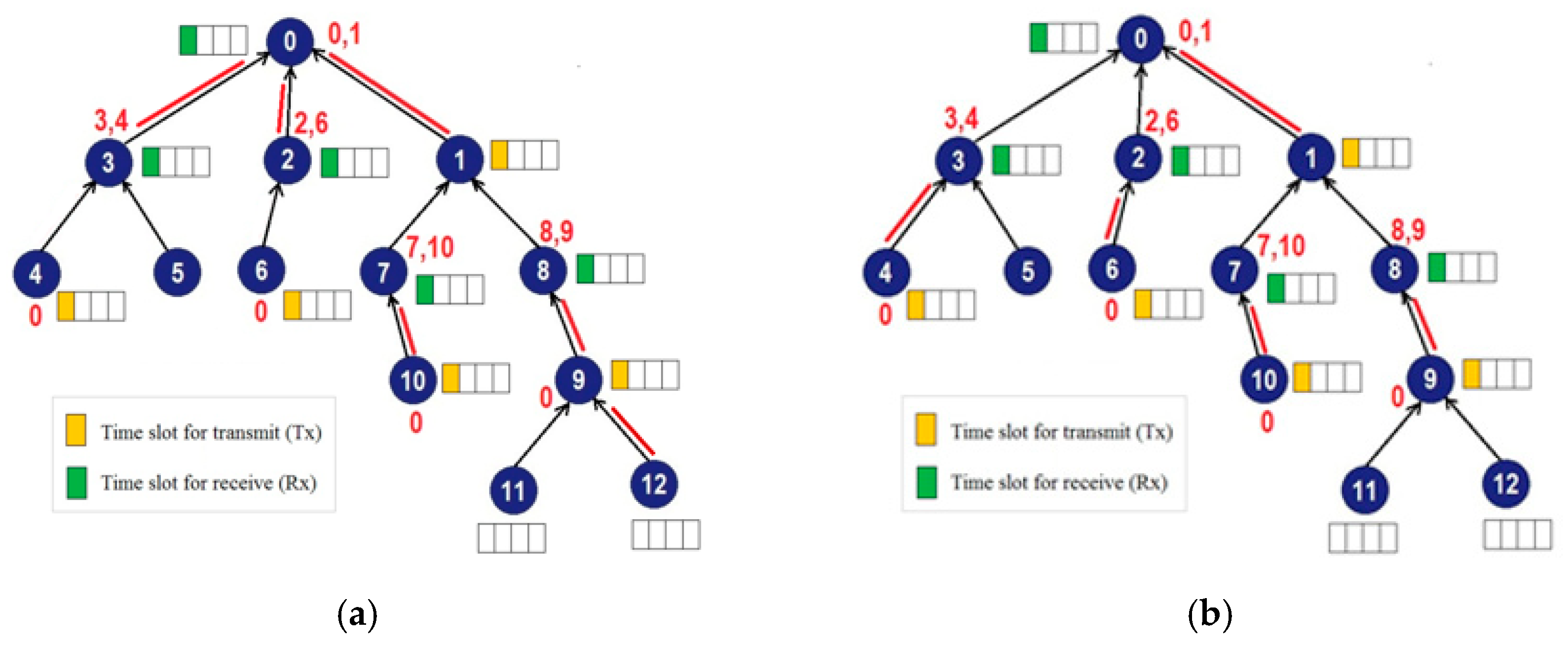
The server knows the overall network conditions, such as the network topology, the number of nodes in the network, and the number of packets waiting in the queue of each network node.

(b)

Each node can synchronize itself to the network and know the schedule to transmit, receive, and sleep, based on information sent by the server.

(c)

At the beginning of each slotframe, each node generates one packet of data regularly to be sent to the master node.

(d)

Each node will do a bursty transmission when it gets its turn to transmit, so that after the transmit process, the queue in the node becomes empty.

(e)

There is no interference and packet loss.

Henceforth, this paper will be organized according to the following research framework. The first part discusses the introduction, the second part describes related works, the third part explains the theories that underlie this research, the fourth part explains the centralized scheduling algorithm for the IEEE802.15.4e TSCH network, the fifth part describes the TLS-VaD and how to use it, the sixth part discusses testing three centralized scheduling algorithms using TLS-VaD, and the last part is the conclusion of the study.

2. Related Works

In addition to the research of [12,13], there is a number of studies that examine the TSCH centralized scheduling algorithm, directly related to TASA or not. There are studies directly related to TASA [14,15,16], and studies not related to TASA [17,18]. Specific to [12,13], this research refers to studies conducted by Shreedar [19] and Sayenko [20]. Shreedar et al. provide an example of how a scheduling algorithm is built and tested for its performance, while Sayenko’s study introduces the term “scheduling decision”, which is one of the topics discussed in this research.

The latest research that refers to TASA was conducted by Meng et al. [14], who produced a scheduling algorithm called matching scheduling algorithm optimization of MSA (MSA-OSA), which has almost the same characteristics as IRByTSA. The only difference is that MSA-OSA gives transmission priority to leaf nodes, while IRByTSA gives transmission priority to high-ranking nodes. Nonetheless, the research conducted by Meng does not discuss the achievement of duty cycles that can be generated by MSA-OSA. It also does not discuss the mechanism of multihop data transfer to be collected at the master node. To test the scheduling algorithm they created, Meng et al. did not mention the use of simulators or specific programming languages. Other research that refers to TASA is a study conducted by Ojo et al. [15], who developed a scheduling algorithm for TSCH networks to maximize energy efficiency. The scheduling algorithm was developed using the energy consumption model on TSCH nodes and nonlinear programming (NLP). However, similar to [14], the study conducted by Ojo et al. also did not mention the simulator/tool used in their research.

Some studies that examined the 802.15.4e TSCH network were conducted by Choi et al. [17], Livolant et al. [18], and Khoufi [21]. In Reference [17], a centralized scheduling algorithm called centralized link scheduling (CLS) was proposed, which utilized the RPL routing protocol to produce its scheduling decisions. The target of this research was to make scheduling algorithms that required fewer control messages. To test the performance of the proposed CLS algorithm, Choi et al. used an OPNET simulator. However, this research did not clearly describe how the OPNET simulator was used to carry out the tests. Meanwhile, Livolant et al. [18] examined the signaling mechanism of the multichannel optimized delay timeslot assignment (MODESA) centralized scheduling algorithm, comparing the number of messages needed to install and upgrade a scheduling scheme on the TSCH network. However, they did not explain what simulators or software were used to do the testing. Research by Khoufi et al. [21] examined the mechanism of TSCH network formation and how long it took to form a network, using the NS3 simulator as a performance test tool against the proposed mechanism. That study showed that NS3 had a TSCH module even though it did not have sufficient support for the development of a centralized scheduling algorithm.

One of the aims of this research was to develop a research support tool. To explain how the tool was designed, written, and developed, this research referred to the work of Felicetti et al. [22] and Beshay et al. [23]. The research of Felicetti et al. [22] developed a new simulator using the JAVA language with the ability to model an information exchange on a nano scale. This simulator provided a toolkit for simulating any types of nano networks. Nanonetworking is a new interdisciplinary area that combines the materials of nanotechnology, biotechnology, and ICT in one unit of research. The first part of this research explained how this simulator was developed, starting from the identification of the main features of the nanonetwork communication. It then explained the simulator’s architecture, which is comprised of classes, and lastly explained the specific aspects of the simulator’s architecture. Meanwhile, research by Beshay et al. [23] described another types of research support called WiNeTestEr, which is a channel emulator that provides better results than existing commercial products do and is an alternative for wireless device testing. The WiNeTestEr emulator is easier to implement than is the drive test procedure. For the ease of use, WiNeTestEr uses the GUI system in its application. This approach is also used by TLS-VaD.

3. Underlying Theories

3.1. IEEE802.15.4 Standards

IEEE802.15.4 is a standard for personal area networks (PAN) that is low-rate, low-power, and low-cost. In this standard, devices are divided into two types: full function device (FFD) and reduced function device (RFD). An FFD can function as a PAN coordinator, coordinator for part of the network, or ordinary device, whereas an RFD only functions as an ordinary device to send data to the PAN coordinator. The FFD, which acts as a coordinator, besides sending its own data, also functions to forward data sent by the RFD. Network topologies supported by the standard are star (single-hop), cluster tree, and mesh (multihop). In the star topology, all communication can be done only through the PAN coordinator, while in other topologies, communication can be done through several coordinators on a multihop basis. The 802.15.4 standard defines two types of channel access methods: beacon enabled (BE) mode and non-beacon enabled (NBE) mode, where the PAN coordinator ensures which one will be selected as the access method. BE mode uses the superframe structure (see Figure 2), where the slotframe format is determined by the coordinator. Each slotframe is limited by beacons that are generated periodically by the PAN coordinator and divided into 16 slots of the same size. The time between two consecutive beacons is called the beacon interval (BI). The duty cycle principle used in the BE mode can be used for power management [24,25].

Optionally, each superframe can consist of active and inactive periods. In the active period, the nodes communicate with their coordinator, while during the inactive period the nodes enter low-power mode to save energy. The active period can then be divided into the contention access period (CAP) and contention free period (CFP). During the CAP, the CSMA-CA slotted algorithm is used to access the channel, whereas CFP communication uses the TDMA method with a number of guaranteed time slots (GTSs), which are predetermined for each node. There is no superframe in the NBE mode. Thus, the node is always active (energy conservation is delegated to the layer above the MAC protocol) and it uses an unslotted CSMA-CA algorithm to access the channel.

A number of studies have examined the performance of the MAC 802.15.4 protocol, in both BE and NBE modes, so that limitations and deficiencies in the standard have been identified. Some of the limitations and disadvantages of the 802.15.4 standard are explained in [24]. These include unlimited delay, limited communication reliability, no protection against interference or fading, and relay nodes that always require energy. For this reason, the 802.15.4 standard is not suitable for many important scenarios that require stringent requirements in terms of timeliness and/or reliability.

3.2. IEEE802.15.4e TSCH

In 2008, IEEE created the 802.15 Task Group 4e [26] to redesign the MAC protocol in the existing 802.15.4 standard to overcome the deficiencies explained in the previous section. One of the results of the design is the use of a time synchronized channel hopping (TSCH) strategy that is useful for improving transmission reliability and energy efficiency. With these energy-saving and reliable characteristics, the IEE802.15.4e TSCH standard is suitable to be part of the Internet of things protocol stack [27].

The 802.15.4e TSCH technology provides a reliable and energy-efficient transmission because it uses the timeslot (TS) and channel-hopping (CH) methods simultaneously. The timeslot access method will eliminate collisions between active nodes to provide deterministic latency and increase throughput on the application that uses it. In the absence of collisions, it will also save on energy use at each node. The channel hopping mechanism will make each node use different frequencies on each transmission. Channel hopping can reduce the influence of interference and multipath fading to improve communication reliability. Thus, TSCH will increase network capacity, increase transmission reliability, and improve latency, while maintaining duty cycles at a low level [24].

The TSCH standard uses a slotframe structure in its timeslot arrangement. Figure 3 shows an example of a slotframe (S) with 12 timeslot times, with a duty cycle of 50%. Thus, in each slotframe there will be six timeslots (λ) that can be used by nodes to stay active and six timeslots for idle/sleep mode. The smaller the value of the duty cycle, the more efficient the use of energy on the network. The number of timeslots in a slotframe (slotframe size) will determine the repetition frequency of the timeslot and the timing for the nodes to carry out the communication process. The smaller the size of the slotframe, the more chance for nodes to actively send/receive data, with the consequence that the duty cycle will increase. The standard does not specify the size of the slotframe, but depends on its application, the size of the slotframe ranges from 10 to 1000 ts [28]. Within each individual timeslot duration, network nodes have the opportunity to send or receive data, receive or send acknowledgments (ACKs), or sleep. By default, the duration of one timeslot according to the 802.15.4e standard is 10 ms [27].

As previously stated, channel hopping can improve communication reliability, because at each transmission opportunity, the nodes will use different frequencies. The frequencies used are related to the channel offset parameter, ChOff. ChOff is translated into a frequency using Equation (1); by using this equation, channel hopping will occur:

f = F{(ASN + ChOff) mod n_ch}.

(1)

ASN is the absolute slot number, and the ASN value shows the number of timeslots used since the network started operating or since a certain time determined by the PAN coordinator. The ASN value will increase along with the passing of the timeslot used for the process of transmitting and receiving in the network. F is a function realized with a lookup table, containing a set of frequencies that are ready to use. ChOff is the channel offset and n_ch is the number of frequencies available, where 0 ≦ ChOff ≦ (n_ch − 1). In the IEEE802.15.4e standard, the value of n_ch is 16 [27]. The relationship between ASN, S, and slotframe cycle (R) is ASN = (R × S + T), where T is the timeslot number (0 ≦ T ≦ S − 1). To be more clear, we can see the illustration in Figure 4.

Figure 4 shows an example of the timeslot and channel hopping (TSCH) concept with two cycles of slotframes. The active part of the slotframe is marked in orange, while the idle/sleep section is marked in light blue. The figure shows one green cell that occupies timeslot 1 and ChOff 2. According to the IEEE802.15.4e standard, the cell is a link, because the standard states that a link is defined as “the pairwise assignment of a directed communication between devices in a given timeslot on a given channel offset”. The use of the cell/link enables communication between two nodes on the TSCH network. Even if the green cells use the same ChOff and T values, based on Equation (1), the ChOff and T values will produce different frequencies because the ASN values for the two cells are different, i.e., 2 and 14. With different ASN values, the transmit/receive process on the link will use different frequencies, f₁ in cycle 1 and f₂ in cycle 2, which leads to the occurrence of the channel hopping mechanism.

3.3. Link Scheduling

In TSCH networks, the mechanism of scheduling becomes a very important part, because the nodes in the network will be active or sleep according to a predetermined schedule. As for what is meant by scheduling, in this research it is link scheduling, because the things to be set up are the timeslots in each slotframe. The scheduling system will generate a schedule that provides information for each node in what timeslot it must transmit, receive, or sleep. In order to save energy, when it gets a sleep turn, the nodes will turn off the radio system because it requires the most energy [27].

In TSCH networks, scheduling must be designed carefully because it will determine the success of the transmission. As an illustration, Figure 5a shows a network with six nodes, a tree topology network with a directed graph showing the links between nodes and its parents. If node E in the figure has a timeslot to send data to node D, D must be ready to receive the data in that slot. Figure 6b shows an example of an activity schedule for each node, starting from timeslot 0 to timeslot 5, using four offset channels. The assumption used in this example is that each node will send one data packet to the master node (node A) on each slotframe. Within the duration of one slotframe, all data in the network nodes must arrive at the master node. If the schedule in Figure 5b is carried out by the network node in Figure 5a, the process of transmitting, receiving, and collecting data and idling will be as shown in Figure 6.

4. Centralized Scheduling Algorithm for the IEEE802.15.4e TSCH Network

The IEEE802.15.4e standard explains how the MAC layer executes a schedule, but it does not specify how to create/make the schedule. Scheduling can be done by a centralized or distributed system. In a centralized scheduling system, there is special node responsible for generating and maintaining network schedules. This particular node is called master node. Each node on the network reports its latest condition to the master node. The conditions that are reported can contain connectivity information or the amount of data queuing in each node [27]. Information entered at the master node will be the basis for the master node to do scheduling. After the scheduling decision is made, the master node will inform the schedule to all nodes in the network.

As noted in the introduction, there have been many centralized scheduling algorithms for TSCH networks. This section will explain some of the centralized scheduling algorithms that will be tested for performance using the TLS-VaD. The scheduling algorithms are IRByTSA, the first top scheduling algorithm (FTSA), and first leaf scheduling algorithm (FLSA). FTSA and FLSA are relatively simple new algorithms used to compare with IRByTSA. Other researchers who are developing link-scheduling algorithms can use the TLS-VaD as a performance test tool.

4.1. Network Models

In this research, the scheduling algorithm is implemented in a tree topology network represented by a directed graph G = (V, E), where V = {n₀, n₁, ..., n_N-1} is a set of devices, and |V| = N is the total number of nodes in the network. n₀ is the master node (PAN coordinator), and 1 ≤ i ≤ (N − 1) is the i-th generic node on the network (FFD or RFD). Figure 7 shows graph G for a network. The PAN coordinator knows graph G and the traffic load generated by each node, that is, ${\tilde{\mathrm{q}}}_{\mathrm{i}},\forall {\mathrm{n}}_{\mathrm{i}}\in \mathrm{V}$, and i ≠ 0. Each node has (i) a parent node, p_i; (ii) a collection of child nodes, ch (n_i); and (iii) a sub-tree ST (n_i), which is composed of n_i itself and all nodes connected to it via multihop paths.

In Figure 7, it is clear that ST(n₀) represents the entire network, G. Each node is connected to its parent p_i through a dedicated link, (n_i, p_i) ∈ E ⊂ (V × V). Thus, there are a number of links |E| = N − 1. In this study, it is assumed that all links are dedicated to avoiding collisions and reliable links are available. Each node n_i is only connected to its parent p_i even though the node has many neighbors.

4.2. Maximal Matching Algorithm

The Internet of things based on IEEE802.15.4e TSCH requires a link-scheduling algorithm, because only duplex conflict-free links can be allocated to the network nodes [9]. A link is in a duplex conflict condition if it is used by the node that transmits and receives data simultaneously and/or receives data from several child nodes at once. The link used by nodes involved in duplex conflict is called the duplex conflict link (DCL), while the link used by nodes that are free of duplex conflict is called the duplex conflict free link (DCFL). Figure 8 depicts DCLs and DCFLs. In Figure 8a, duplex conflict occurs in the links used by node 0 and node 9, while Figure 8b shows links that are duplex conflict free.

To get DCFLs, the scheduling algorithm in this research uses the graph maximal matching method, which is described as follows:

Maximal matching (G; V; E):

1. M = Ø;

2. While (more edges can be added):

2.1. Starting from the edge that connected to the highest rank node, select an edge, e, which has no vertex in common with an edge in M;

2.2. $M=M\cup e$.

3. Return M.

G is a directed graph with tree topology, V and E are sets of vertex and edge in graph G. M is a set of matching edges on graph G, where M is a subset of E.

4.3. Network Traffic and the Duty Cycle

This research assumes that in each duration of an S-sized slotframe, the n_i node in graph G generates a constant number of packets, that is, ${\tilde{\mathrm{q}}}_{\mathrm{i}}$. The network supports multi-point to point traffic, in which all packets are aimed at the root node, n₀, so that each link (n_i, p_i) is only used for the uplink. Each of these nodes forwards the data packet to the parent p_i node, which eventually will lead all the packets to the master node (PAN coordinator). Assuming that all packets in the node are waiting in the queue at the beginning of the slotframe, this research uses the parameter $\tilde{\mathrm{Q}}$ as a symbol of the total packets that must be sent to the PAN coordinator (n₀) in one slotframe, which can be expressed by Equation (2):

$$\tilde{\mathrm{Q}}={\displaystyle \sum _{\mathrm{i}=1}^{\mathrm{N}-1}{\tilde{\mathrm{q}}}_{\mathrm{i}}}.$$

(2)

It is stated in Section 3.2 that each node on the network cannot transmit and receive simultaneously and receive data from many nodes at once. Therefore, to collect all data in the master node, the transmit and receive processes are needed in stages. All network nodes that have been scheduled to be active by the master node, send/receive the data simultaneously. The simultaneous transmit/receive process will be done in several cycles, until all data in the network reach the master node (n₀). The state that all data have arrived at the master node is marked by the fulfillment of q₀ = $\tilde{\mathrm{Q}}$ condition, where q₀ is the queue size of node 0 (n₀).

To meet the stringent requirements related to packet delay and power consumption, the scheduling algorithm in this study strived for a minimum duty cycle value for each node in the network. To send network traffic of $\tilde{\mathrm{Q}}$ to master node (n₀), the scheduling algorithm will arrange to enable the entire transmission to be carried out in the first λ slot of each slotframe. Since λ ≤ S, the remaining slots of (S − λ) will be left empty, thus leading to the duty cycle of λ/S. If the nodes are evenly distributed on the network, the minimum number of active timeslots (λ) in one slotframe is equal to $\tilde{\mathrm{Q}}$.

4.4. Deepening of the Observed Scheduling Algorithm

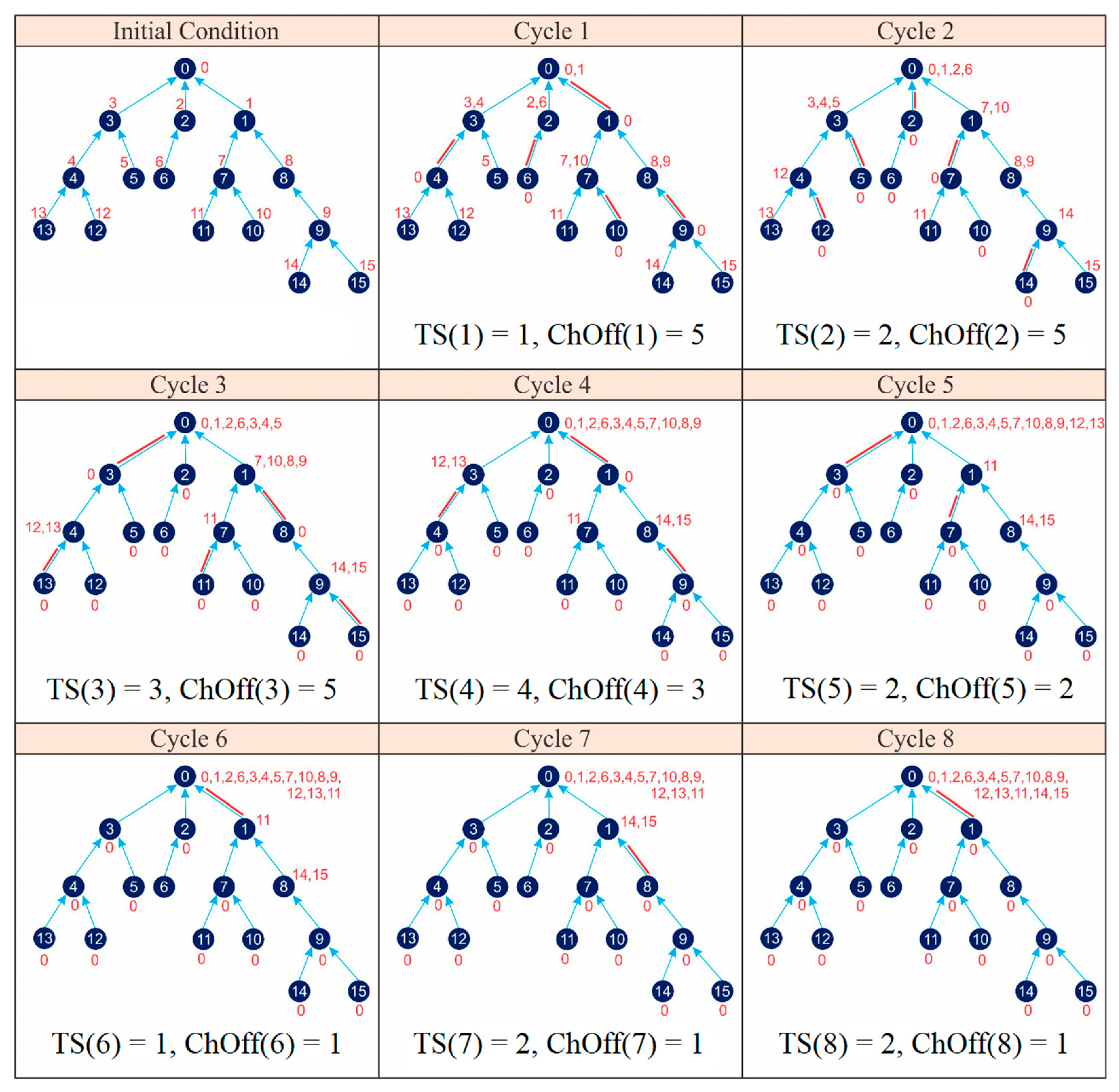
This section explains IRByTSA, FTSA, and FLSA, to make sure that they proceed according to plan when their visualization/animation is displayed by the TLS-VaD. The algorithms were applied to networks with topology as shown in Figure 9.

As an introduction,

Table 1. Comparison of Iman–Ramli bursty transmission scheduling algorithm (IRByTSA), first top scheduling algorithm (FTSA), and first leaf scheduling algorithm (FLSA).

No	Item	IRByTSA	FTSA	FLSA
1	Process of generating scheduling decisions is done on/for each timeslot	No	No	No
2	Bursty transmission	Yes	Yes	Yes
3	Transmission priority on the network	From higher-rank node	From higher-rank node	From leaf node
4	Transmission priority based on queue size of a node	No	No	No
5	Transmission priority based on number of child nodes	No	No	No
6	Resource allocation is only given to nodes with qn ≠ 0	Yes	Yes	Yes
7	Chance to transmit from child to parent node based on turn	Yes	No	No

provides a summary of the three scheduling algorithms to highlight their similarities and differences. It can be seen in item 2 of the table that all three algorithms used the bursty transmission mechanism. As for what is meant by bursty transmission, when a node gets a chance to transmit, the node will send all the data in its queue. Thus, with a scheduling algorithm that uses the principle of bursty transmission, every chance to transmit is an opportunity to empty the queue.

Since IRByTSA, FTSA, and FLSA apply the bursty transmission principle, the relationship between λ and the number of cycles (C) is formulated in Equation (3) as follows:

$$\mathsf{\lambda }={\displaystyle \sum _{\mathrm{s}=1}^{\mathrm{C}}\mathrm{TS}\left(\mathrm{s}\right)},$$

(3)

where TS (s) is the number of timeslots needed for each cycle (s) and variable C states the number of cycles needed to send all data to the master node, so that condition q₀ = $\tilde{\mathrm{Q}}$ can be achieved. TS(s) is determined by Equation (4), as follows:

$$\begin{gathered} \mathrm{TS}\left(\mathrm{s}\right)={\max \{\mathrm{ts}}_{\mathrm{i}}{\left(\mathrm{s}\right)|\mathrm{n}}_{\mathrm{i}}\in \mathrm{Active}\left(\mathrm{s}\right)\} \\ ={\max \{\mathrm{q}}_{\mathrm{i}}{\left(\mathrm{s}\right)|\mathrm{n}}_{\mathrm{i}}\in \mathrm{Active}\left(\mathrm{s}\right)\}. \end{gathered}$$

(4)

Equation (4) implies that ts_i(s) = q_i(s), where ts_i(s) represents the total timeslot needed by n_i for transmitting data in step/round (s) and q_i(s) is the number of packets queued in n_i in a given round s. This is an applicable formula because: (a) the TSCH network requires one timeslot to send one data packet, and (b) the node that receives a transmit turn will do bursty transmission when sending its data. Thus, the number of timeslots needed by each node will be equal to the number of packets in the node’s queue. Active(s) in Equation (4) indicates a set of nodes that are active at a particular cycle(s). Based on Equation (4), TS(s) will take the largest q_i(s) value from Active(s). This is done to ensure that the number of timeslots allocated at each cycle meets the needs of all nodes that are scheduled to be active (sending or receiving data). If the value of TS(s) is smaller than the number of packets that are queuing at the nodes, even only one node, then not all nodes will be able to do bursty transmission because the number of allocated timeslots is insufficient.

4.4.1. IRByTSA

Prior to the discussion of IRByTSA, it is necessary to look at

Table 2. Variables used in IRByTSA.

Variables	Description
G	Graph representation
ND	Total number of nodes in the network
NCD[i]	Number of child nodes of node [i]
TS(s)	Number of timeslots needed for each cycle (s)
$\tilde{\mathrm{Q}}$	Total number of packets in network nodes waiting to be sent to master node within 1 slotframe duration
i	Node number
y	Turns
s	Cycle/iteration
qz	Queue size in node z
turn_now[i]	Refers to one child of node i that gets a transmission turn at a particular cycle/iteration
child_of_node[i][j]	j-th child node of node i
child_number_of[i][z]	The function that will produce a number showing the sequence number of node z as a child node of node i.
mod_node[i]	Value used for modulus operations on node i, used to enable child nodes to send data to node i alternately (no priority)
Matching_link[s]	Variable that stores the set of active links in each cycle/iteration (s)

, which shows the symbols used in this algorithm.

A flowchart of IRByTSA is presented in Figure 10, while the explanation for the algorithm is as follows:

1

IRByTSA starts with a flowchart symbol, as shown in Figure 11. Once we start the program, we will see several variables. G is a graphic representation of the tree topology network, as shown in Figure 9.

2

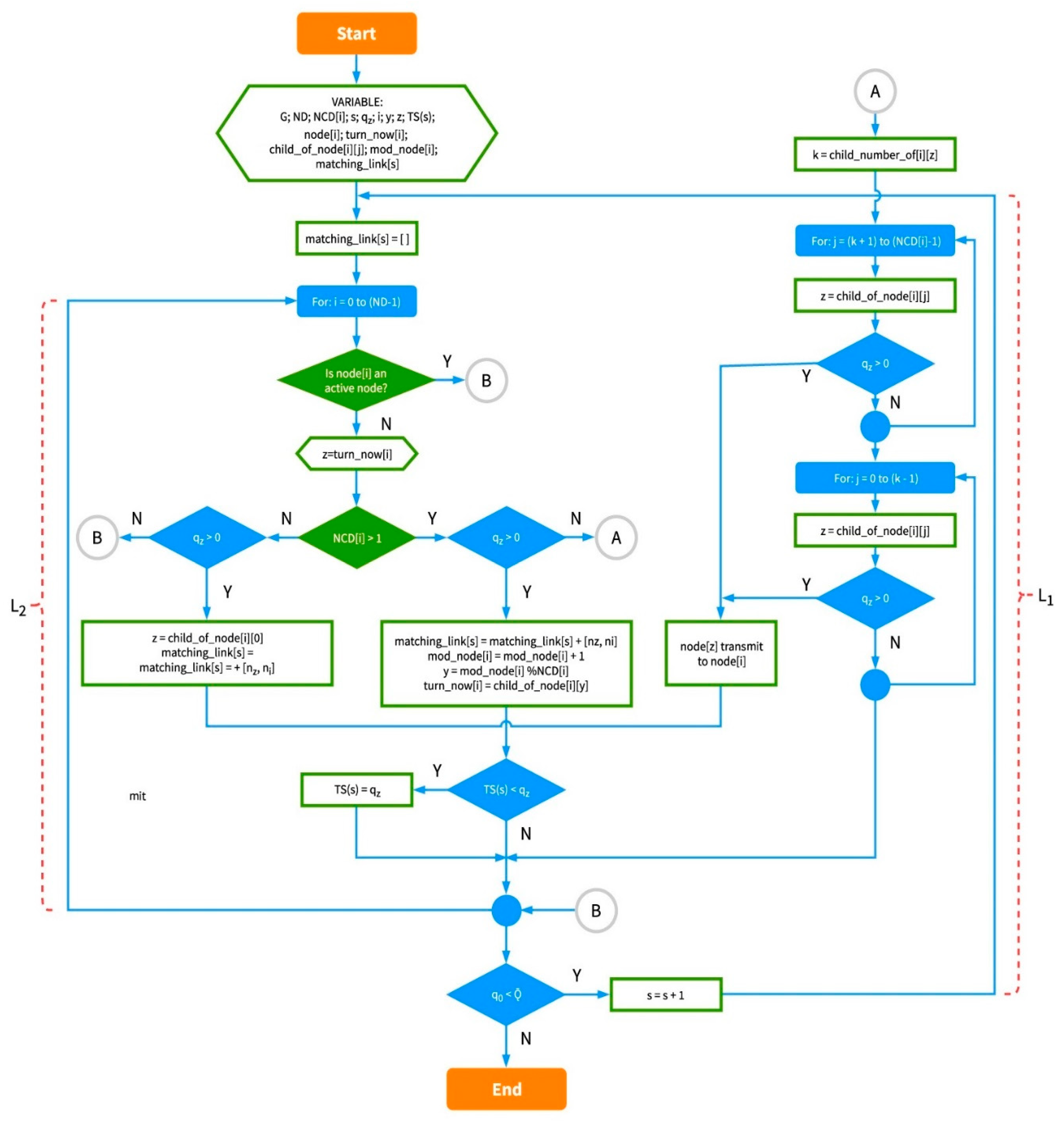
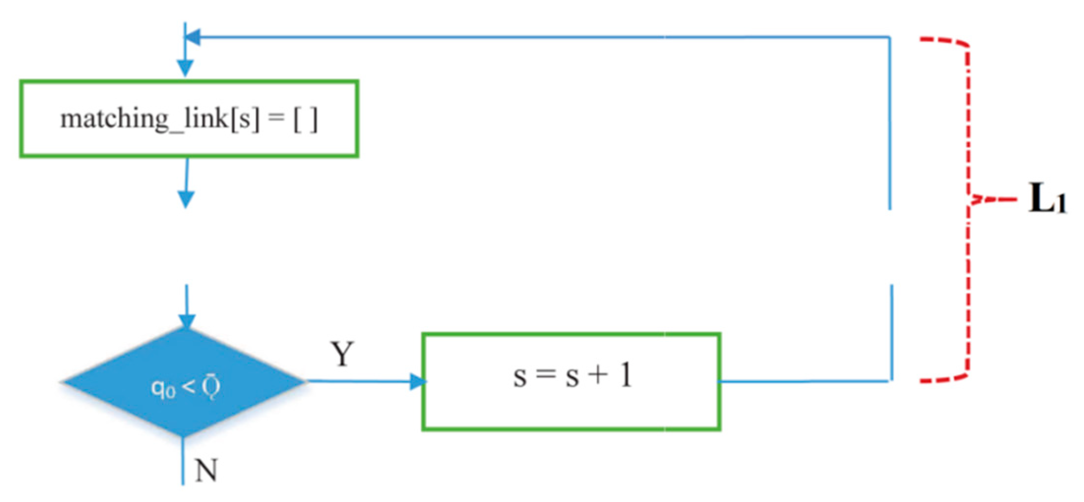
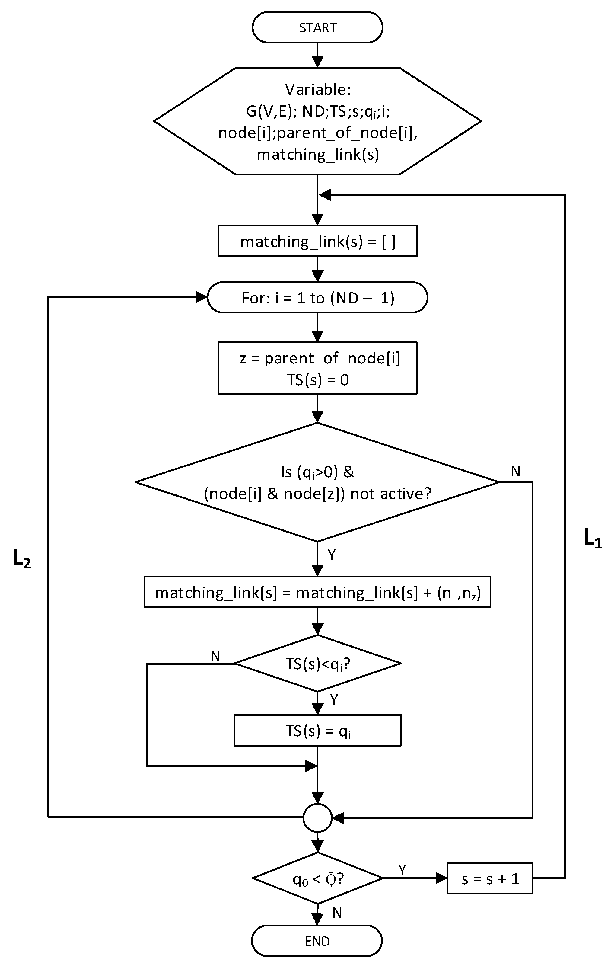
IRByTSA contains two loops/iterations, L₁ and L₂, where L₂ is inside L₁. The continuity of the looping process in L₁ is determined by the condition q₀ < $\tilde{\mathrm{Q}}$, as shown in Figure 12.

Meanwhile, the L₂ loop is controlled by the symbol shown in Figure 13. In the L₂ loop, the iteration symbol For: i = 0 to (ND – 1) states that the scheduling will process all nodes in the network, starting from node 0 to node (ND – 1).

3

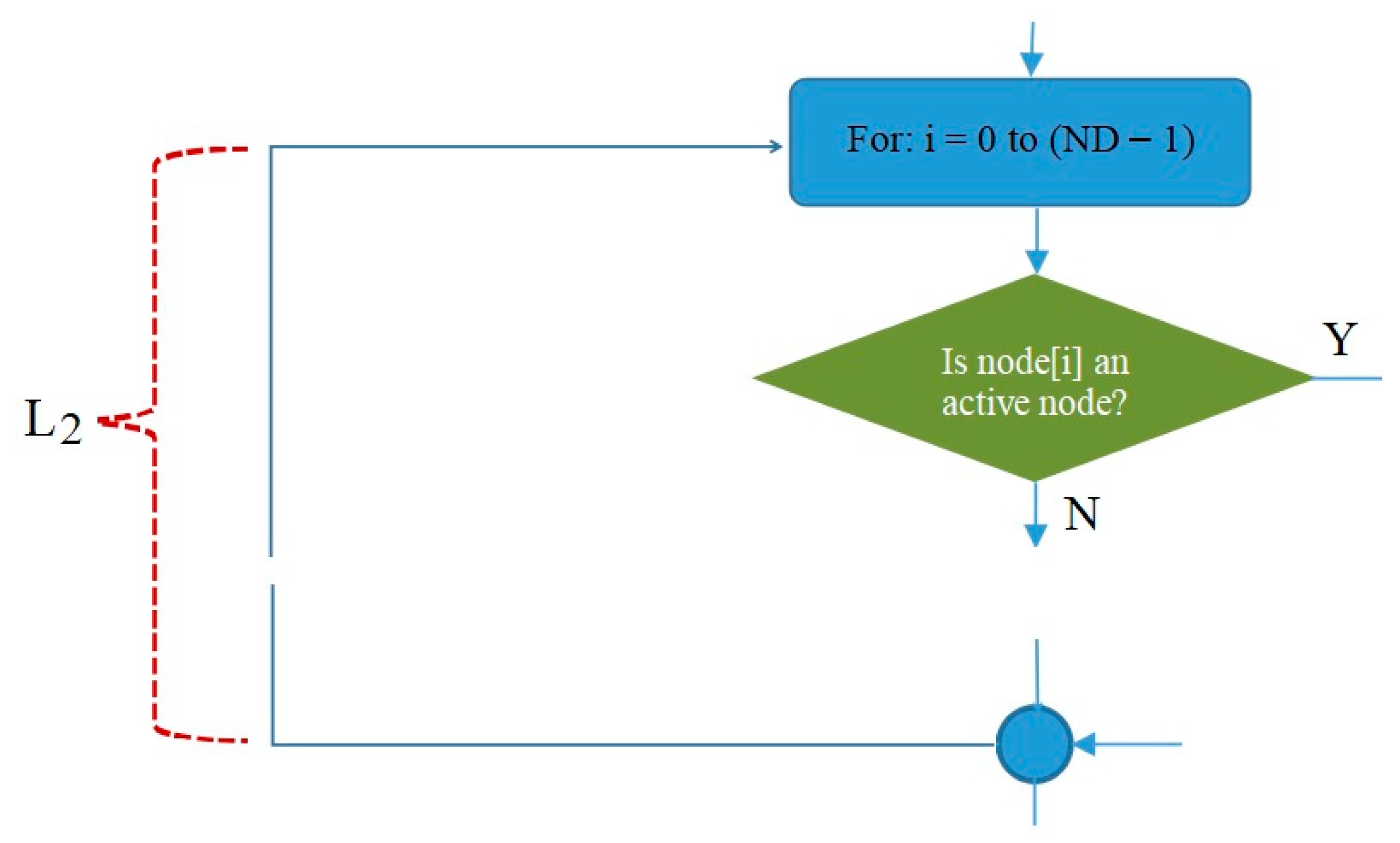
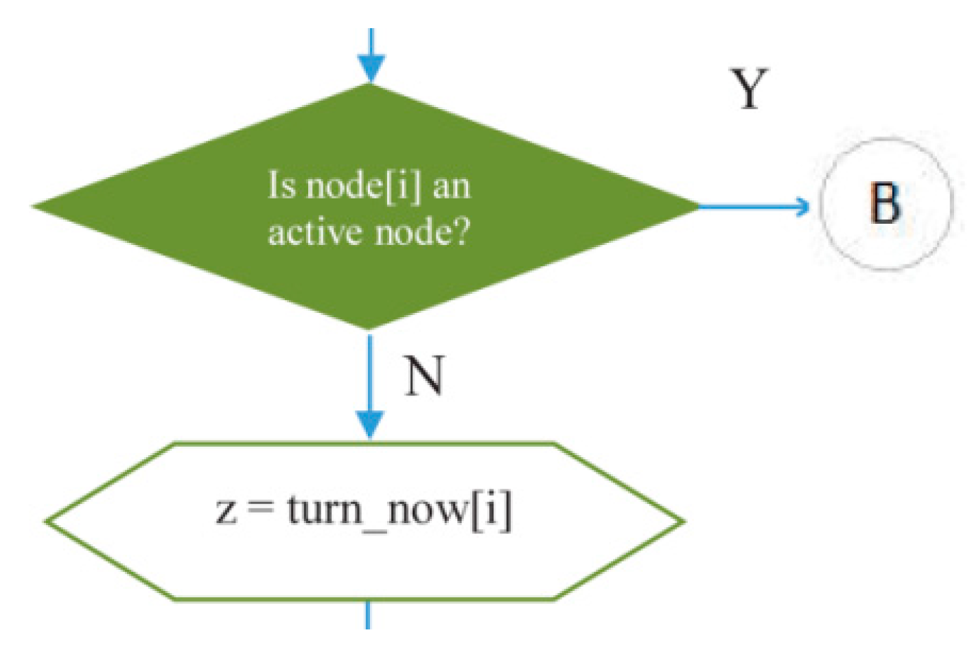
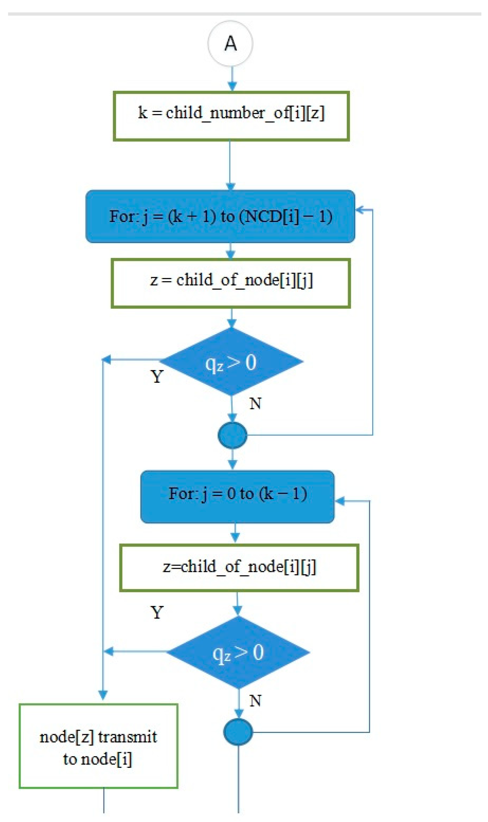
The decision-making symbol in Figure 14 is used to indicate that if at a certain cycle/iteration node i is not active (because it has not had a turn to transmit or receive), one of the children of node i will get a turn to transmit. Meanwhile, if node i is active, the iteration in L₂ will continue to node (i + 1) until all inactive nodes in the network get a turn to transmit or receive. In this way, the principle of graph matching will be realized in this scheduling algorithm.

The variable turn_now [i] is used to indicate which child of node i will be given a turn to transmit as long as the child node has data in its queue. The child number of node i is contained in variable z.

4

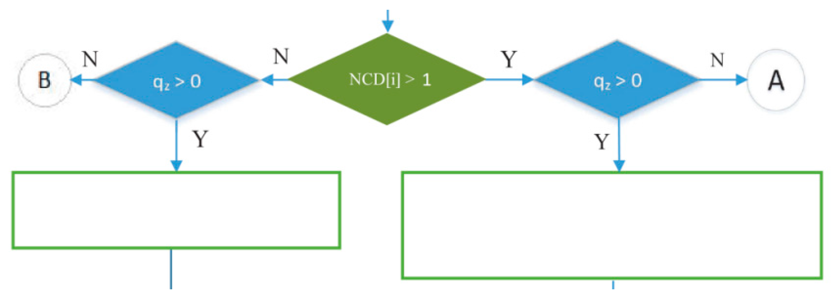
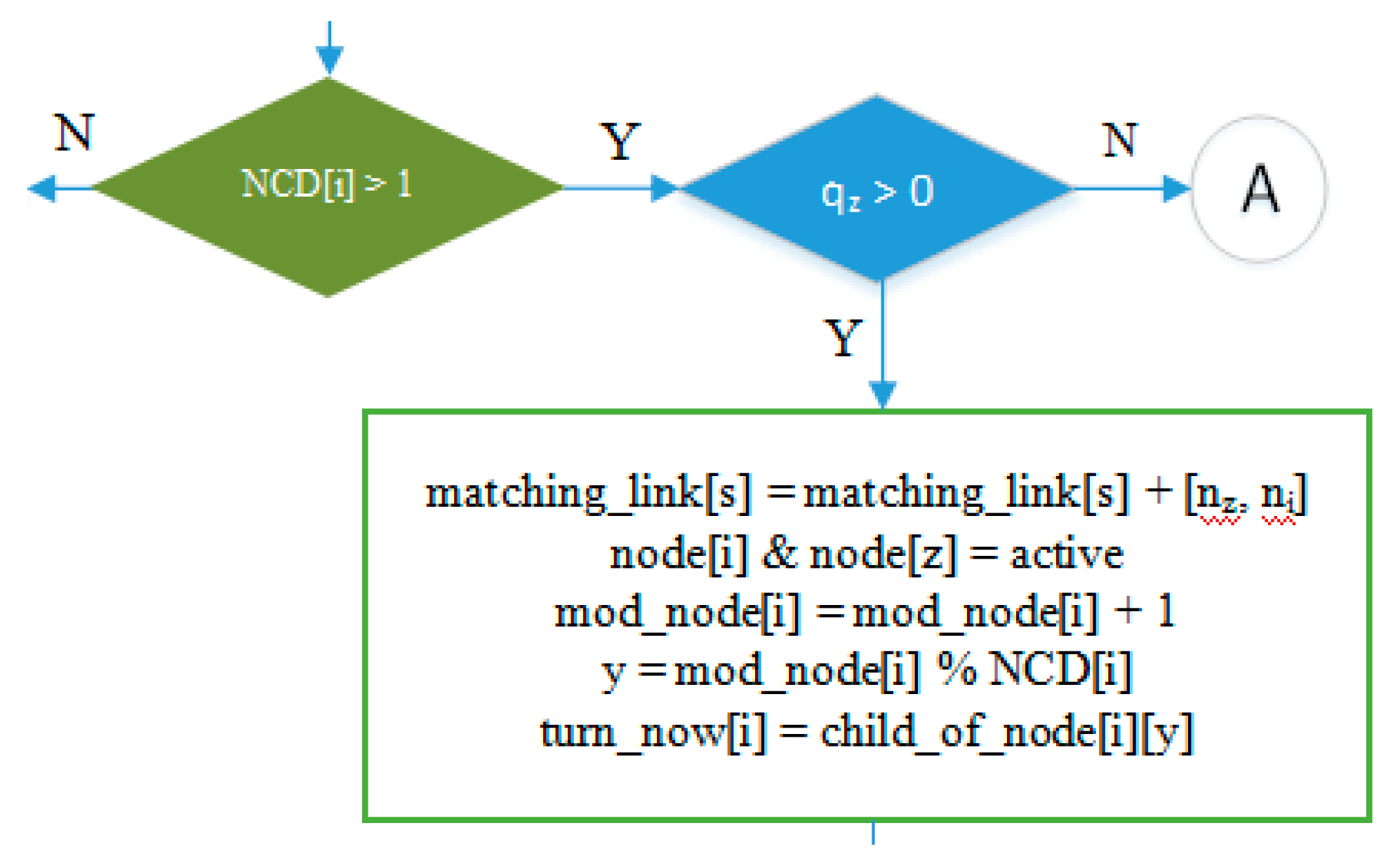
The green decision symbol in Figure 15 is used to indicate whether node i has more than one child or not. If node i has more than one child, it will proceed to the blue decision symbol on the right, and if it only has one child, it will proceed to the left. Meanwhile, the two blue decision symbols are used to determine whether the queue is empty at the child node of node i.

5

Part of the IRByTSA flowchart in Figure 16 states that if node i has more than one child (NCD [i] > 1) and the child of node i has a transmit turn (node z) and its queue is not empty (q_z > 0), then node z is given the opportunity to transmit to node i, as indicated by the command line matching_link[s] = matching_link[s] + [n_z,n_i].

Meanwhile the following line of code:

mod_node[i] = mod_node[i] + 1

y = mod_node[i] % NCD[i]

turn_now[i] = child_of_node[i][y],

is used to give each child of node i, as long as it still has data to send, a transmit turn alternately. The turn_now[i] variable is used to store information related to the turn. Thus, supposing we have turn_now [10] = 5 in a cycle, the child of node 10 that gets the transmit turn is node 5.

If node i has more than one child (NCD [i] > 1) and the child of node i has a transmit turn (node z) and its queue is empty (q_z = 0), the transmit turn will be given to another child of node i. If no child of node i has data to send, the scheduling process will continue for node (i + 1). The flowchart section in Figure 17 describes these steps.

6

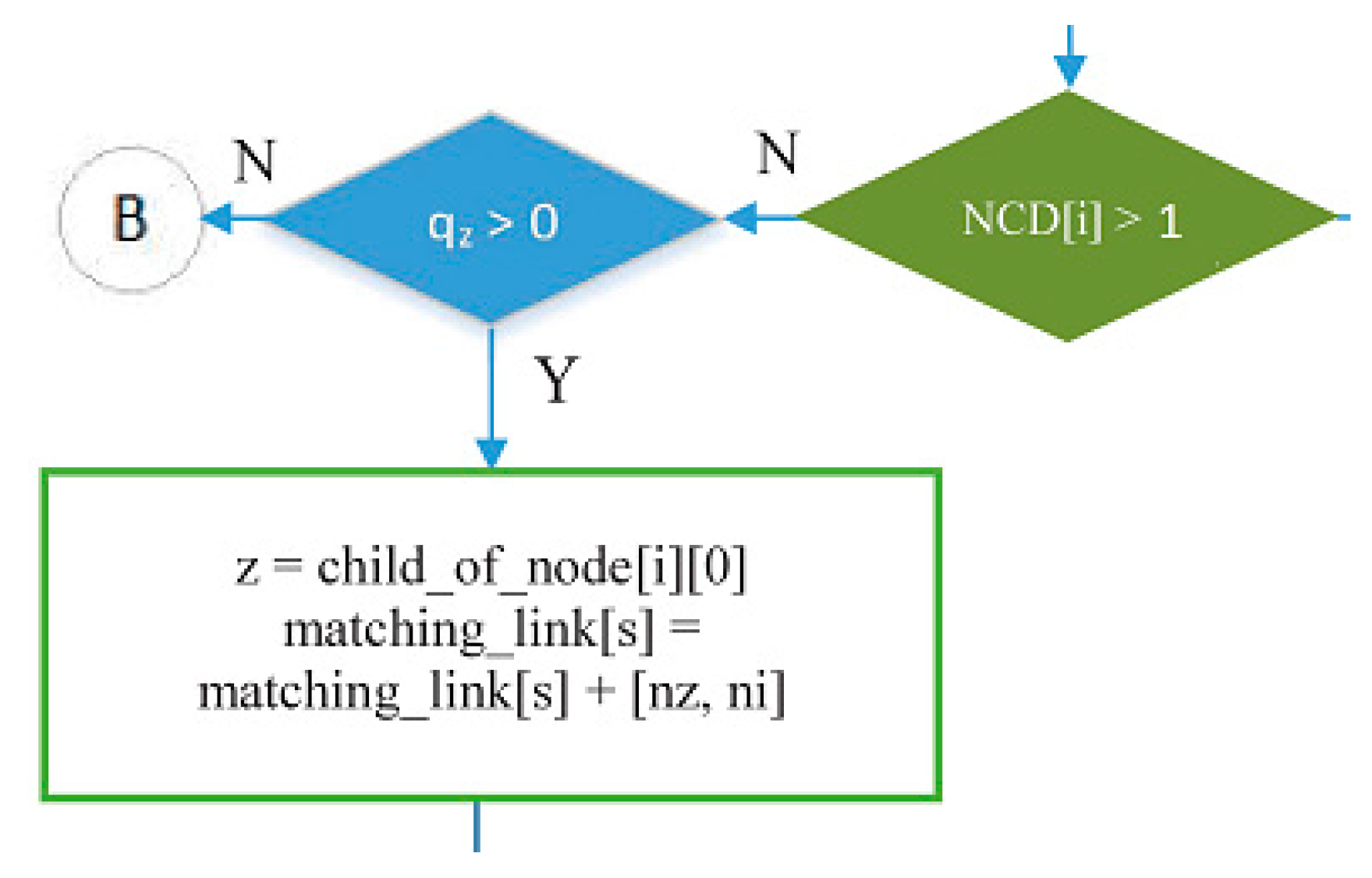
If node i only has one child node and it has data to send, the child node (n_z) will be scheduled to transmit data to its parent (n_i), indicated by the command line matching_link[s] = matching_link[s] + [n_z,n_i]. Figure 18 shows the part of flowchart that illustrates that step.

7

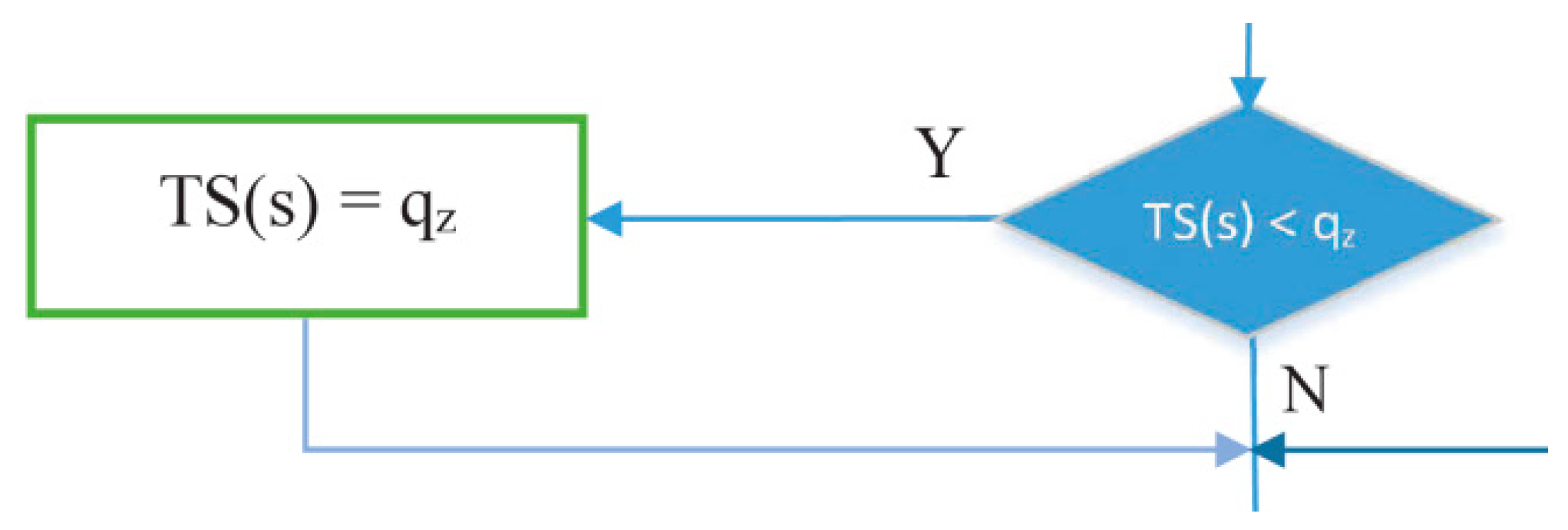
The part of the flowchart in Figure 19 is used to find the node that has largest number of packets to be sent in a cycle (s), since the number of packets indicates the number of timeslots needed. IRByTSA looks for the largest timeslot value required by active nodes in each cycle (s) to ensure that the number of timeslots allocated meets the transmission needs of all active nodes.

Figure 20 shows the application of IRByTSA on the 16-node network shown Figure 9. Figure 20 illustrates the steps, starting from the initial condition where each node has one packet waiting to be transmitted, and it continues with the process of sending packets gradually to the master node. IRByTSA requires eight cycles to collect all data in the master node.

Based on Figure 20, we could determine the values of parameters C, λ, and total channel offsets (ChOffs) required if we used IRByTSA as in the following:

◆

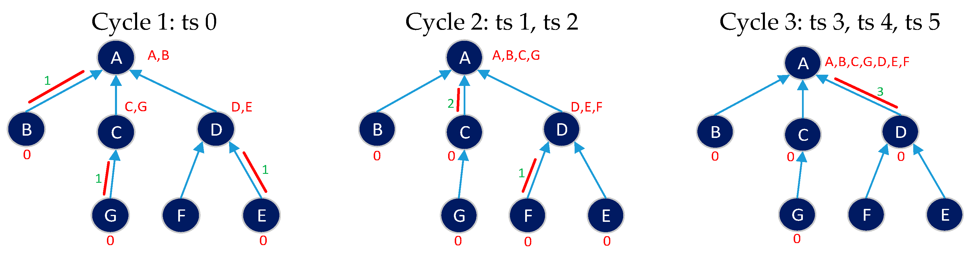
C_IRByTSA = 8 cycles;

◆

$\mathrm{Total}\mathrm{ChOff}={\displaystyle \sum _{s=1}^{C}ChOff(s)}$ = ChOff(1) + ChOff(2) + ChOff(3) + ChOff(4) + ChOff(5) + ChOff(6) + ChOff(7) + ChOff(8) = 5 + 5 + 5 + 3 + 2 + 1 + 1 + 1 = 23 ChOffs;

◆

${\mathsf{\lambda }}_{\mathrm{IRByTSA}}={\displaystyle \sum _{\mathrm{s}=1}^{\mathrm{C}}\mathrm{TS}\left(\mathrm{s}\right)}$ = TS(1) + TS(2) + TS(3) + TS(4) + TS(5) + TS(6) + TS(7) + TS(8) = 1 + 2 + 3 + 4 + 2 + 1 + 2 + 2 = 17 timeslots.

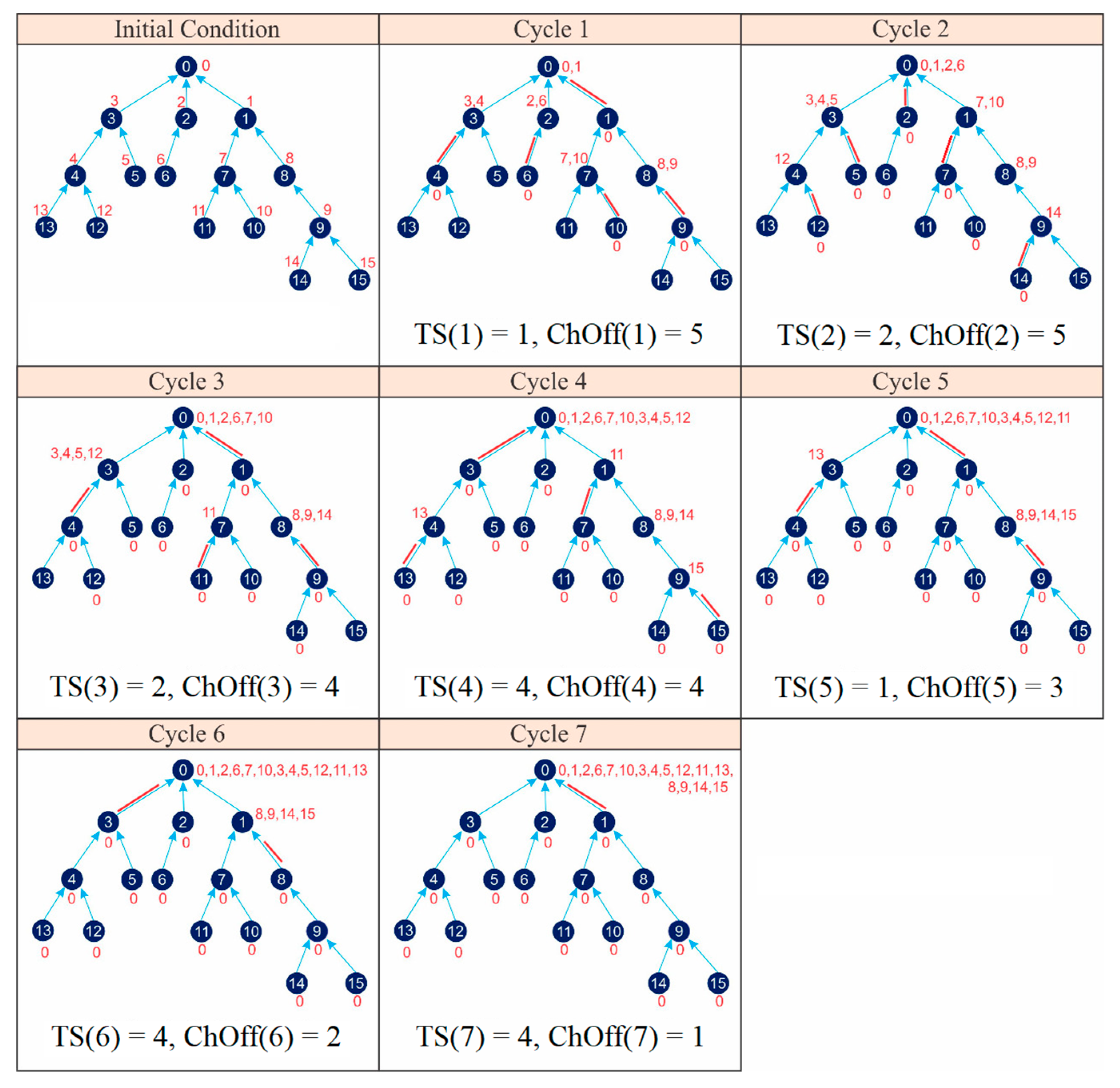
4.4.2. FTSA

The FTSA is the first comparison for IRByTSA. This algorithm has a simpler structure than IRByTSA, as shown in Figure 21. Table 1 shows that the difference between FTSA and IRByTSA only lies in item 7, particularly in the process of providing transmission opportunities between child nodes to its parent, be it based on turn or not. The sequence of FTSA child nodes that are given the chance to transmit is always fixed or not based on turn. The transmission chance in each cycle always starts from the same node as long as the node has data, while in IRByTSA, the opportunity to transmit is given to the child nodes based on turn.

Just like the IRByTSA, the FTSA will provide output in the form of matching_link(s) containing the schedule for each node in each cycle. Figure 22 shows both active and idle/sleep nodes in each cycle by leaning on the matching_links(s) generated by the FTSA. Figure 22 enables us to determine the values of parameters C and λ if we use the FTSA:

◆

C_FTSA = 7 cycles;

◆

$\mathrm{Total}\mathrm{ChOff}={\displaystyle \sum _{s=1}^{C}ChOff(s)}$ = ChOff(1) + ChOff(2) + ChOff(3) + ChOff(4) + ChOffS(5) + ChOff(6) + ChOff(7) = 5 + 5 + 4 + 4 + 3 + 2 + 1 = 24 ChOffs;

◆

${\lambda }_{FTSA}={\displaystyle \sum _{s=1}^{C}TS(s)}$ = TS(1) + TS(2) + TS(3) + TS(4) + TS(5) + TS(6) + TS(7) = 1 + 2 + 2 + 4 + 1 + 4 + 4 = 18 timeslots.

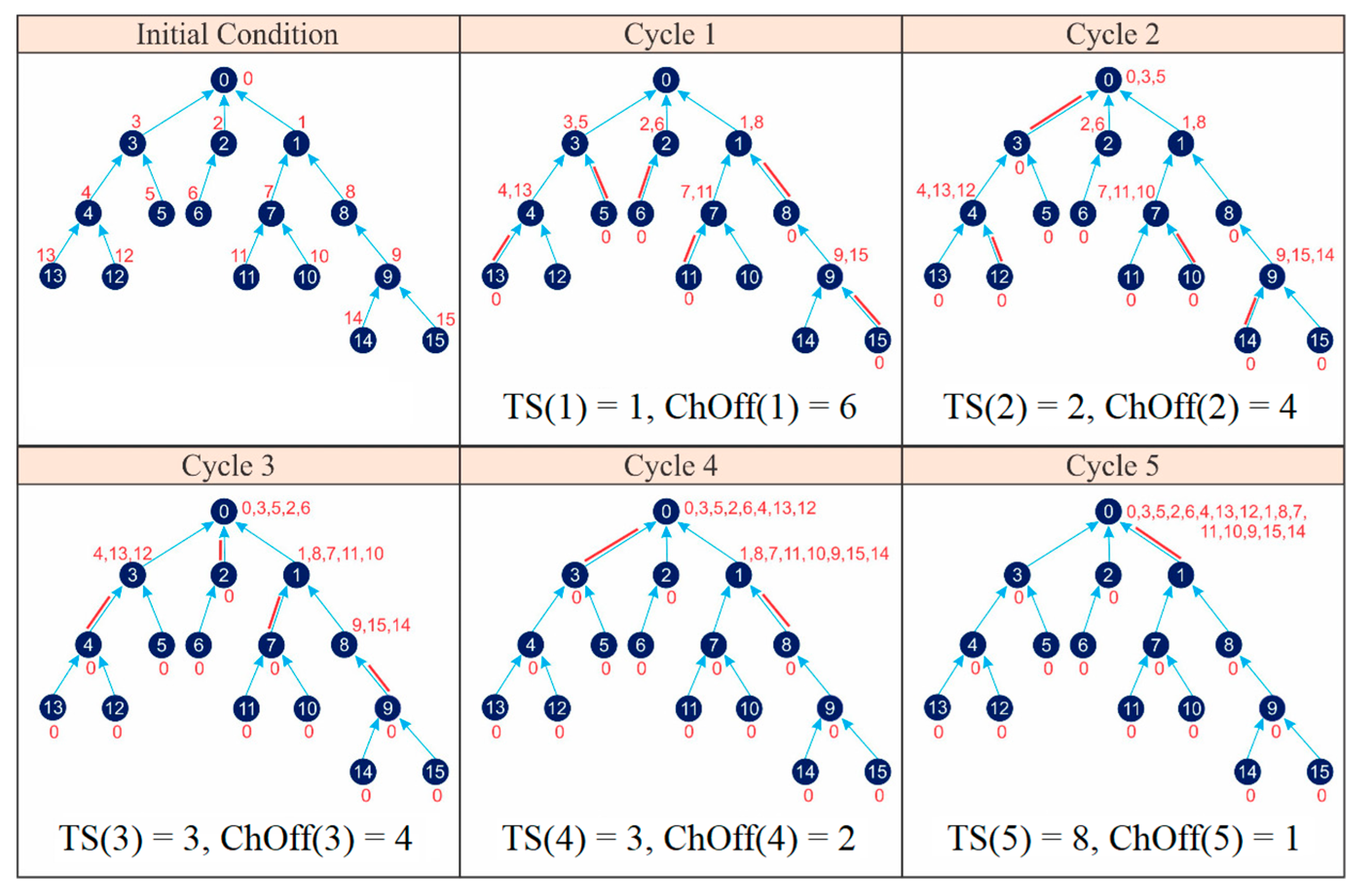
4.4.3. FLSA

The FLSA is the second comparison for IRByTSA. Just like FTSA, FLSA has a simpler structure than IRByTSA, as indicated by the flowchart in Figure 23. As illustrated in Table 1, FLSA differs from IRByTSA in only two ways: (1) its transmission turn always starts from the leaf node, and (2) at each cycle, the order of transmission from the child node to its parent is always fixed, and the chance of transmission always starts from the same node as long as the node has data.

The algorithm output is schedule information summarized in the matching_link (s) variable. The schedule information will be announced by the master node to all nodes in the network to inform them about the timeslot when the nodes must be active or idle/sleep. Figure 24 shows the active and idle/sleep nodes in each cycle based on matching_links (s) generated by the FLSA.

From Figure 24 the values of parameters C and λ can be determined if the TSCH network uses the FLSA:

◆

C_FLSA = 5 cycles;

◆

$\mathrm{Total}\mathrm{ChOff}={\displaystyle \sum _{s=1}^{5}ChOff(s)}$ = 6 + 4 + 4 + 2 + 1 = 17 ChOffs;

◆

${\lambda }_{FLSA}={\displaystyle \sum _{s=1}^{C_{FLSA}}TS(s)}$ = TS(1) + TS(2) + TS(3) + TS(4) + TS(5) = 1 + 2 + 3 + 3 + 8 = 17 timeslots.

To compare the performance of IRByTSA, FTSA, and FLSA, we recapitulated the results of the algorithm test for small networks in

Table 3. Temporary recapitulation of the scheduling algorithm performance.

Scheduling Algorithm	Active Timeslots (λ)	Cycles (C)	Total Channel Offsets (ChOff)
IRByTSA	17	8	23
FTSA	18	7	24
FLSA	17	5	17

. In terms of the number of active timeslots (λ) and number of cycles, the table indicates that the performance of FLSA was better than that of IRByTSA and FTSA, while IRByTSA’s performance was slightly better than FTSA’s. However, to draw conclusions about which of these scheduling algorithms has the best performance in terms of the λ or duty cycle parameters and the number of cycles, we need further testing on networks with larger dimensions. Therefore, we continued performance testing of these three algorithms by measuring their performance on a larger network. The testing used the TLS-VaD to hasten the process.

5. TSCH Link Scheduling Visualization and Data Processing

Research in the field of network protocol requires simulators as a tool for visualization, validation, and performance testing, and one of the research topics in this field is scheduling algorithms. Studies of scheduling algorithms commonly use NS-2, NS-3, OPNET, and other simulators. However, the centralized scheduling algorithm on TSCH has very few supporting simulators, including NS-3 [29] and 6TiSCH simulator [30], which only provide limited support. Therefore, this research seeks to develop a tool for developing a centralized link-scheduling algorithm on the IEEE802.15.4e TSCH network. We succeeded in making a tool known as the TSCH link-scheduling visualization and data processing or abbreviated as TLS-VaD. The TLS-VaD was developed to meet the following objectives:

❖

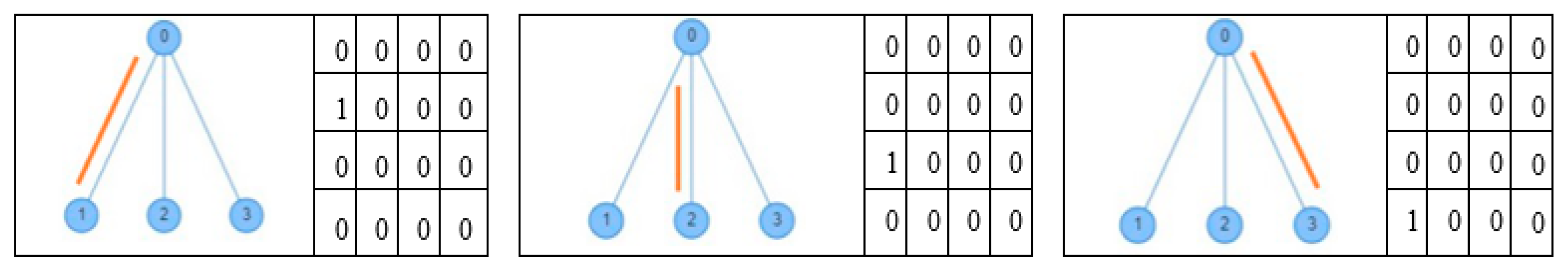
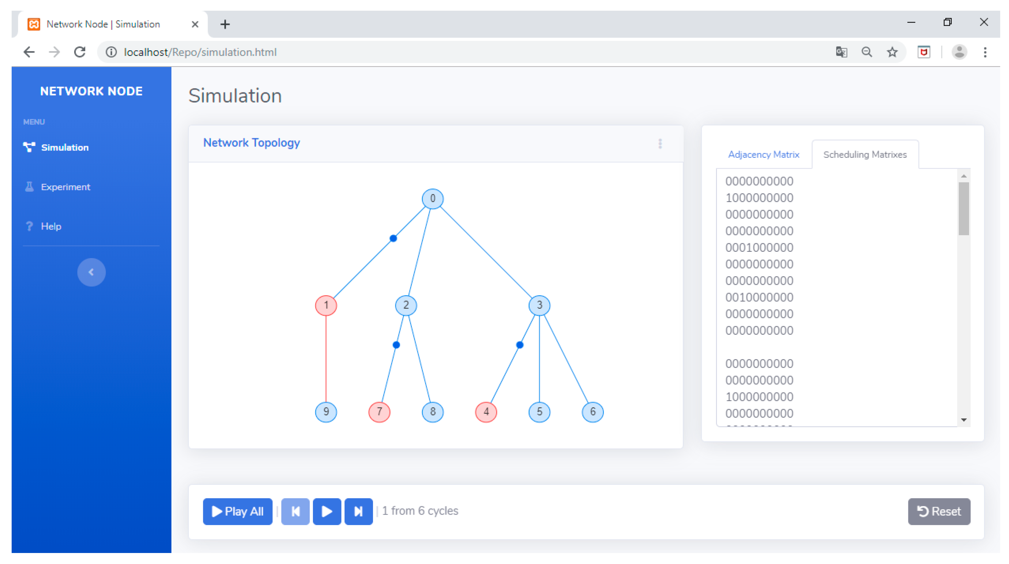
It visualizes the transmit and receive processes between nodes in a network in a number of cycles. The data in the nodes of each cycle will move toward the master node gradually. Information on which nodes are active in each round is determined by the schedule matrices generated by the scheduling algorithm. With this visualization, researchers can determine whether the developed scheduling algorithm is in accordance with the plan or not.

❖

It provides data output that shows the performance of the developed scheduling algorithm: number of active timeslots per slotframe (λ), number of cycles (C) and duty cycles (DC), and number of required channel offsets (ChOffs). The output of this tool will show the following performance:

■

Number of active timeslots per slotframe (λ): the fewer active timeslots, the shorter the on time of network nodes, thereby saving on the amount of energy used.

■

Number of cycles: indicates the speed of the scheduling algorithm in generating schedules. The smaller the number of cycles, the faster the algorithm can create a schedule. In terms of centralized network management, the faster the schedule, the better, because the resources to create the schedule can be used to serve other networks.

■

Duty cycle: number of active timeslots when connected to the size of the slotframe. At the same slotframe size, the smaller the duty cycle, the better, because it indicates a network condition that is increasingly energy-efficient.

■

Required channel offset: used to get the channel offset per cycle (ChOff/C) parameter. ChOff/C shows the average number of channel offsets used in each cycle. Since the 802.15.4e standard only provides 16 channel offsets, the ChOff/C value should be smaller than 16. The smaller the ChOff/C value, the better, because it will reduce the possibility of interference with other nodes that are active at the same time/cycle. Even though this research assumes there is no interference, it is still important to note ChOff/C data as preliminary information for researchers who want to include interference problems as a parameter to consider.

❖

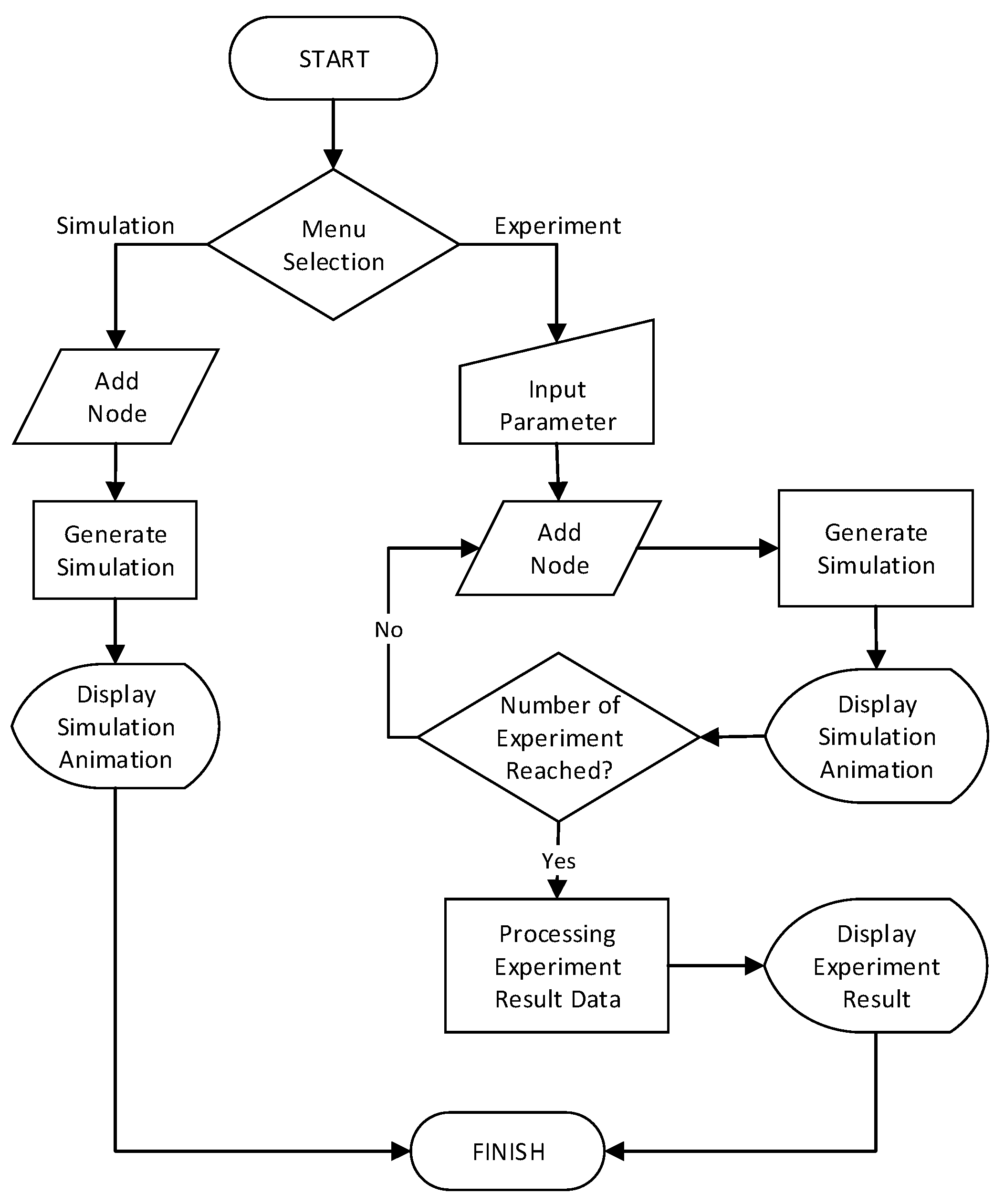
It provides a platform for researchers in the field of centralized link-scheduling algorithms to test the performance level of developed algorithms. A scheduling algorithm has good performance if all output data released from TLS-VaD has a minimum value. If we want to improve the performance of the algorithm, it can be repaired separately, because in order to use TLS-VaD, researchers can simply create an executable (exe) file from the developed algorithm and embed the file on TLS-VaD. Since TLS-VaD only requires exe files, researchers do not need to be bound to one particular programming language; they only need to create an exe file capable of processing input in the form of an adjacency matrix and producing schedule matrices as output. These schedule matrices will then be processed by TLS-VaD to produce animations and data output. A description of the relationship between TLS-VaD and the exe file of the scheduling algorithm is presented in Figure 25.

5.1. The Design of TLS-VaD

5.1.1. System Design

TLS-VaD is an open platform for anyone who wants to observe the performance of a scheduling algorithm. To observe or examine an algorithm, all users of TLS-VaD must have an executable file of the algorithm to be observed. The use case diagram for this tool can be seen in Figure 26, which shows that the application contains two main feature: simulation and experiment. The simulation feature will visualize the process of transmitting and receiving the data on a network that is controlled by a scheduling algorithm. Whereas with the experiment feature, besides being able to see animations, users can also obtain data that are related to the performance of the selected scheduling algorithm.

The activities that are carried out in the simulation feature can be seen in Figure 27, which shows that to obtain the desired results, user must first enter the network topology. Network input can be done by either drawing node by node or by inputting the adjacency matrix of the network. After accomplishing the input process, the next activity is applying the scheduling algorithm and the running animation procedure to the network. As for the experiment feature, Figure 28 shows that the activities that must be carried out are almost the same as those for the simulation feature. The difference lies in that the experiment feature also includes a process for inputting the network topology iteratively as well as a process for displaying experimental data.

As stated in the previous section, to test a scheduling algorithm using TLS-VaD, researchers must attach the executable file of the scheduling algorithm to be observed. The processes of developing the algorithm and the programming language used are left to each researcher. For success with TLS-VaD, researchers must abide by the following rules: (1) the attached executable file must be able to accept input in the form of an adjacency matrix that represent the network topology (see Figure 29). The digit 1 in the matrix shows a connection between a pair of nodes where its node number corresponds to the row and column numbers of the digit. (2) The attached executable file must be able to produce scheduling matrices that represent the activities of transmitting and receiving data at nodes in the network. The number of matrices shows the number of cycles needed to send all data to the master node (see Figure 30 for more details).

5.1.2. Implementation

This tool was designed and built using the following website-based programming technologies:

• Native PHP (hypertext processor): A technology for creating basic scripts that are widely used for website-based applications.
• C ++: the programming language used in this software for processing input data in the form of a matrix that is transformed into the software using a multi-dimensional array.
• Javascript: a high-level programming language that runs on the client-side like a browser. Here, it was used to create animations/visualizations.
• HTML (hypertext markup language): a markup language that is used to make the main structure of the display of web-based software.
• Bootstrap: a CSS framework that is used for HTML styling so that the software display becomes neater and more attractive.
• Animate traffic: this library, which was created using Javascript, displays animation from input data in the form of arrays. Here, it was used as a library to display animation/visualization.

The flowchart that illustrates how the TLS-VaD works as a whole can be seen in Figure 31.

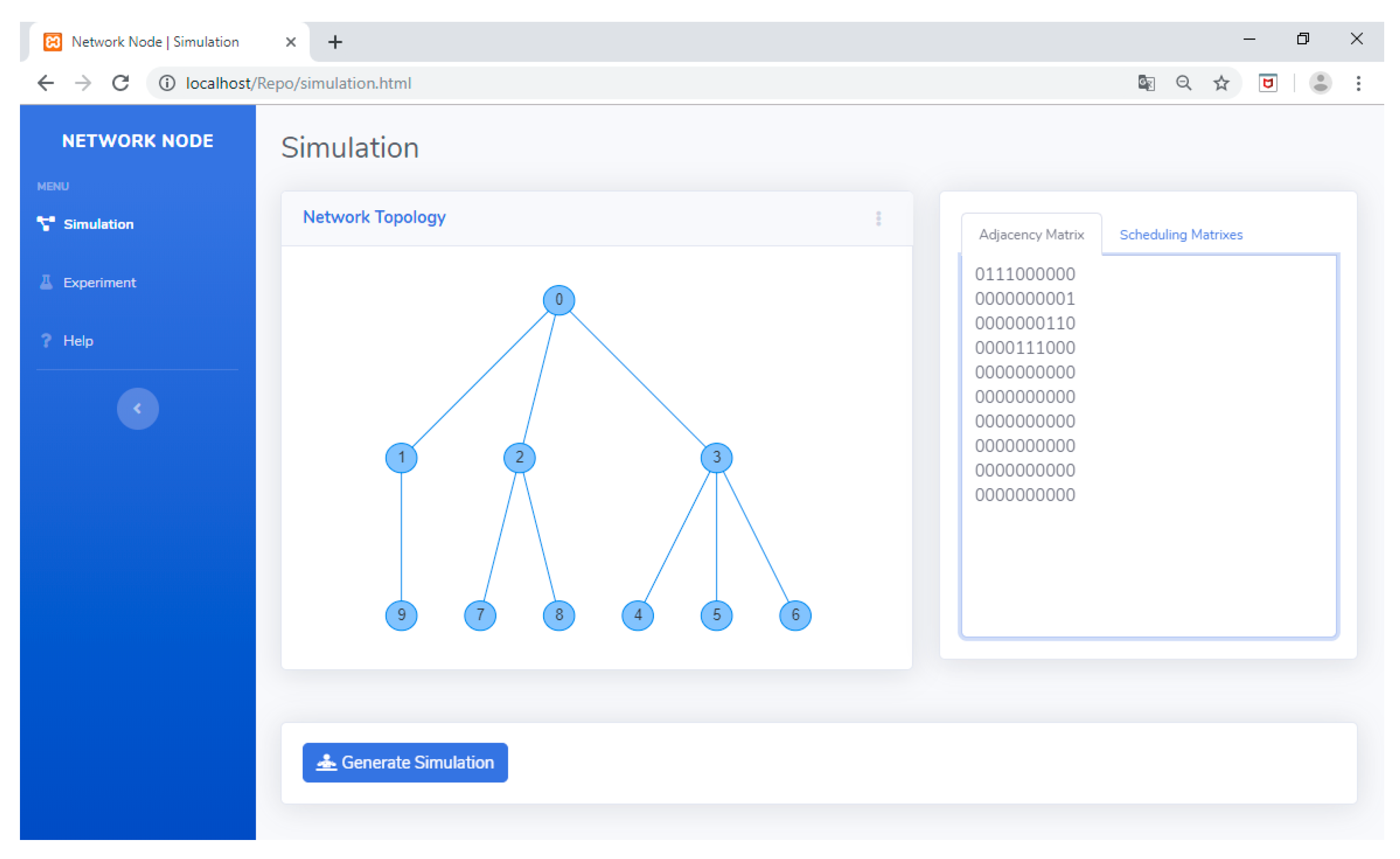
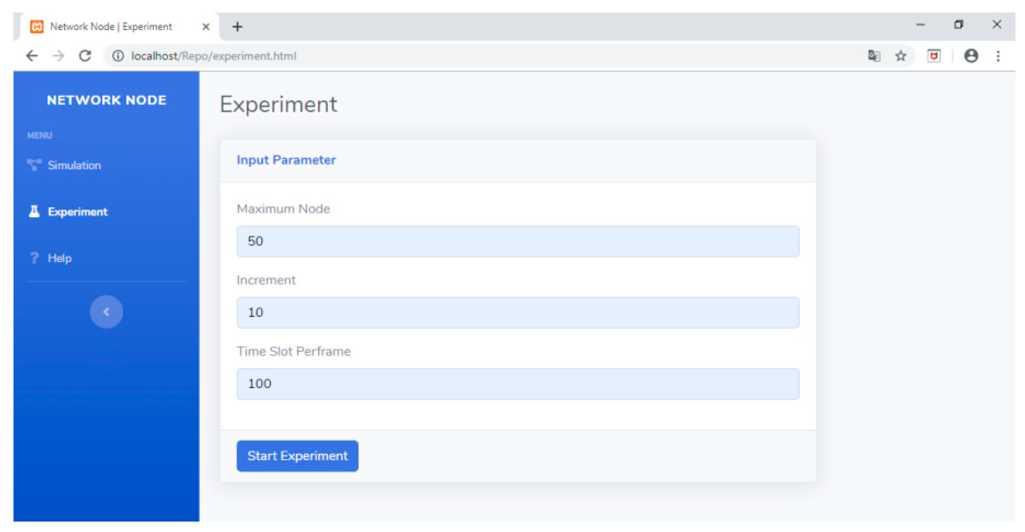
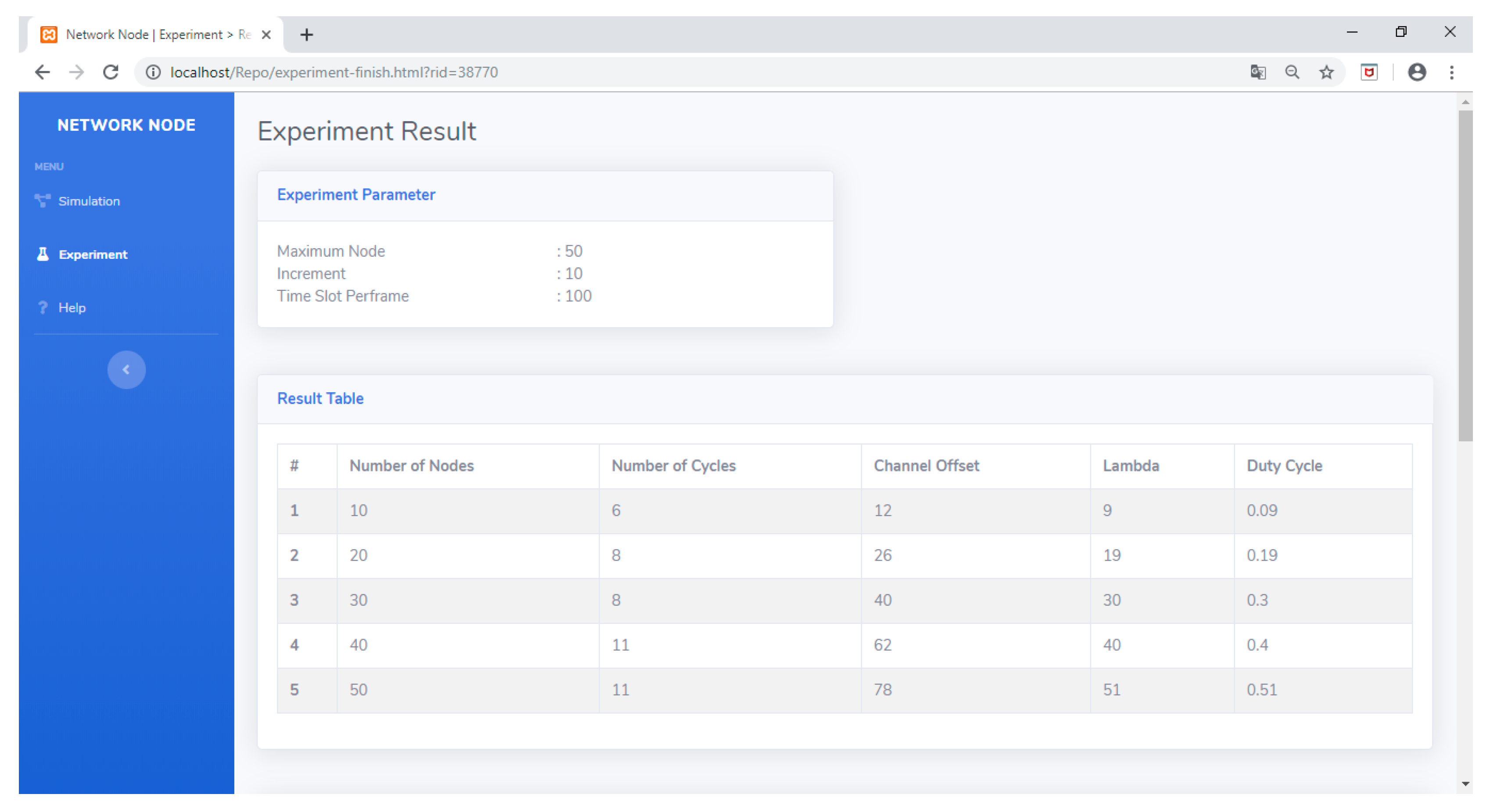
5.2. Using the TLS-VaD

To make this tool easy to use and more interesting, TLS-VaD uses a GUI in its application. Figure 32 shows the display of TLS-VaD. This tool provides two menus (simulation and experiment), and two input system (network topology and adjacency matrix). As mentioned in Section 5.1, the simulation menu is used to test whether the algorithm being designed is running as planned, while the experiment menu is used to obtain data so that we can measure the performance of a scheduling algorithm. Figure 32 shows the network topology that was entered into the network topology section, and the adjacency matrix section shows the relevant adjacency matrix.

If the user selects the simulation menu, then after entering the input, he/she can press the generate simulation button to see the animation or visualization of the transmit and receive processes in the network (see Figure 33). Figure 33 shows red and blue nodes in the network, with red indicating a node with an empty queue and blue indicating a node with a queue filled with packets waiting to be sent. Figure 33 shows no nodes that transmit and receive activities simultaneously and no node that receives data from child nodes simultaneously. Sending data from child nodes to their parents is done alternately. To ensure that the designed algorithm runs as planned, we could observe the transmit and receive processes at each cycle, which could be played back using the Play All, Play, Rewind, and Forward buttons.

Meanwhile, if the user is in the experiment menu, then the user will be guided to enter the desired experiment scenario. Figure 34 shows the display when the experiment scenario is entered. After the scenario is determined, the data collection process can be commenced by pressing the Start Experiment button. The results of the experiment will bring up the data summarized in the result table. Figure 35 shows the result table containing data about the number of cycles (C), channel offset (ChOff), active timeslots (λ), and duty cycle (DC) for network dimensions ranging from 10 to 50 nodes. These data allow researchers to analyze the performance of the developed scheduling algorithm.

6. Scheduling Algorithm Performance Test Using TLS-VaD

In this section, the TLS-VaD was used to compare the performance of IRByTSA with FTSA and FLSA. A good link-scheduling algorithm in TSCH networks has the following characteristics:

(a)

It results in minimum values for active timeslots (λ) and duty cycles (D).

(b)

It is quick at generating scheduling decisions that are marked by a minimum cycle (C) value.

Active timeslot (λ) has minimum magnitude if its value is equal or close to $\tilde{\mathrm{Q}}$, while the speed in generating scheduling decisions is indicated by the number of cycles (C) in Equation (3). The smaller the value of C, the faster the algorithm generates scheduling decisions.

6.1. Hypotheses on the Performance of Scheduling Algorithms

This section explains some hypotheses related to the performance of each scheduling algorithm, as follows:

(a)

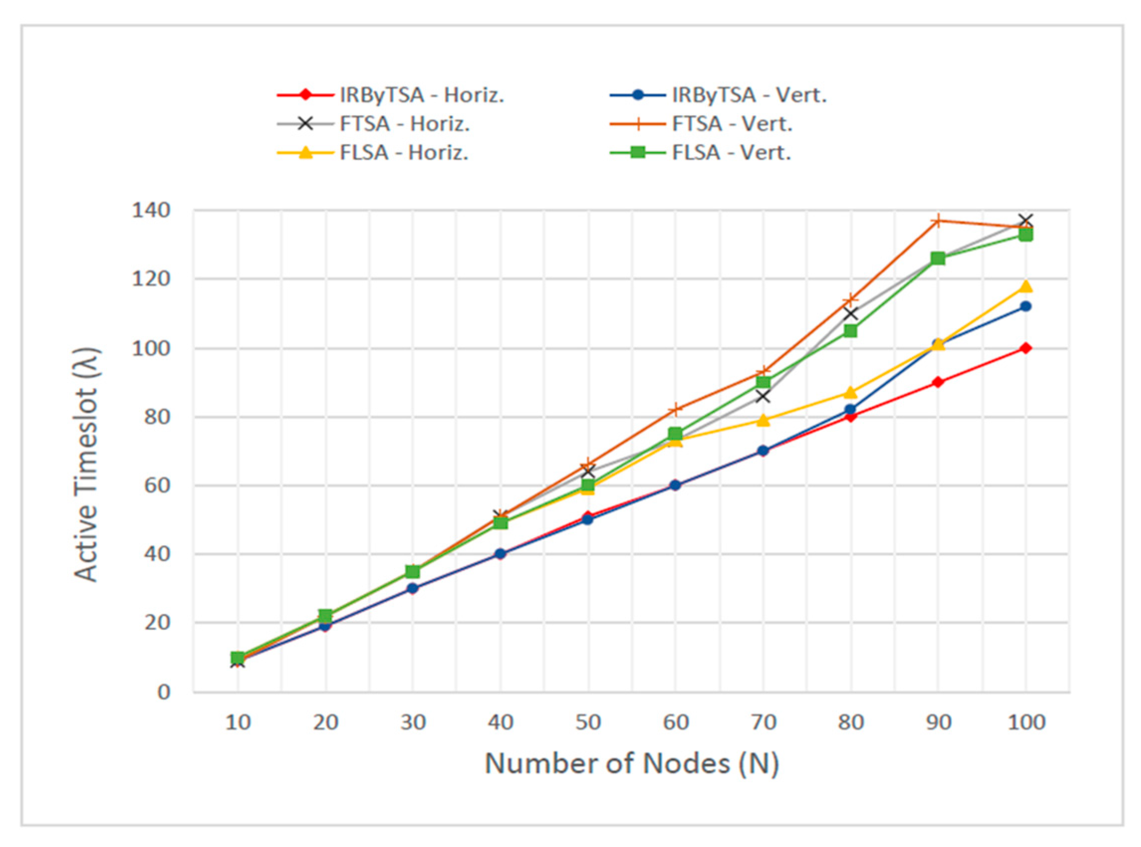
In producing minimum λ, IRByTSA will outperform FTSA and FLSA. This is estimated because IRByTSA prioritizes transmission at higher-rank nodes. By prioritizing higher-rank nodes, data packets will arrive at the master node faster, which decreases the number of timeslots needed to send data along the passing of cycles. The decreased need for timeslots in each cycle will produce the minimum λ value.

(b)

In producing the minimum number of cycles, FLSA will outperform IRByTSA and FTSA. This can occur because FLSA gives priority to transmission at leaf nodes that will give more links to the DCFL(s) than the algorithm that prioritizes transmission at higher nodes. With more links on DCFL(s), network data will reach the master node faster. Faster arrival of data at the master node on a network that uses FLSA will be reflected in fewer cycles than a network that uses IRByTSA or FTSA.

(c)

In producing a minimum λ, FTSA will not perform as well as IRByTSA, because in FTSA, the opportunity to transmit from the child node to its parent is not done in rotation, resulting in a buildup of data at certain nodes, leading to increased λ value generated by the algorithm.

(d)

In producing a minimum number of cycles, FTSA will not perform as well as FLSA because of two factors: (i) transmission priority is given to higher nodes. Algorithms that give priority to transmission at higher nodes will not be able to provide more DCFLs than algorithms that give priority to transmission at leaf nodes. Thus, what happens to IRByTSA will also happen to FTSA. (ii) The process of transmitting from a child node to its parent always starts from the first child node, not based on turns. As long as the child nodes have data, even if only one data packet, the node will be given the opportunity to transmit. This will result in data reaching the master node slowly, so the number of cycles needed to collect all data at the master node will be greater than the number of cycles in IRByTSA and FLSA.

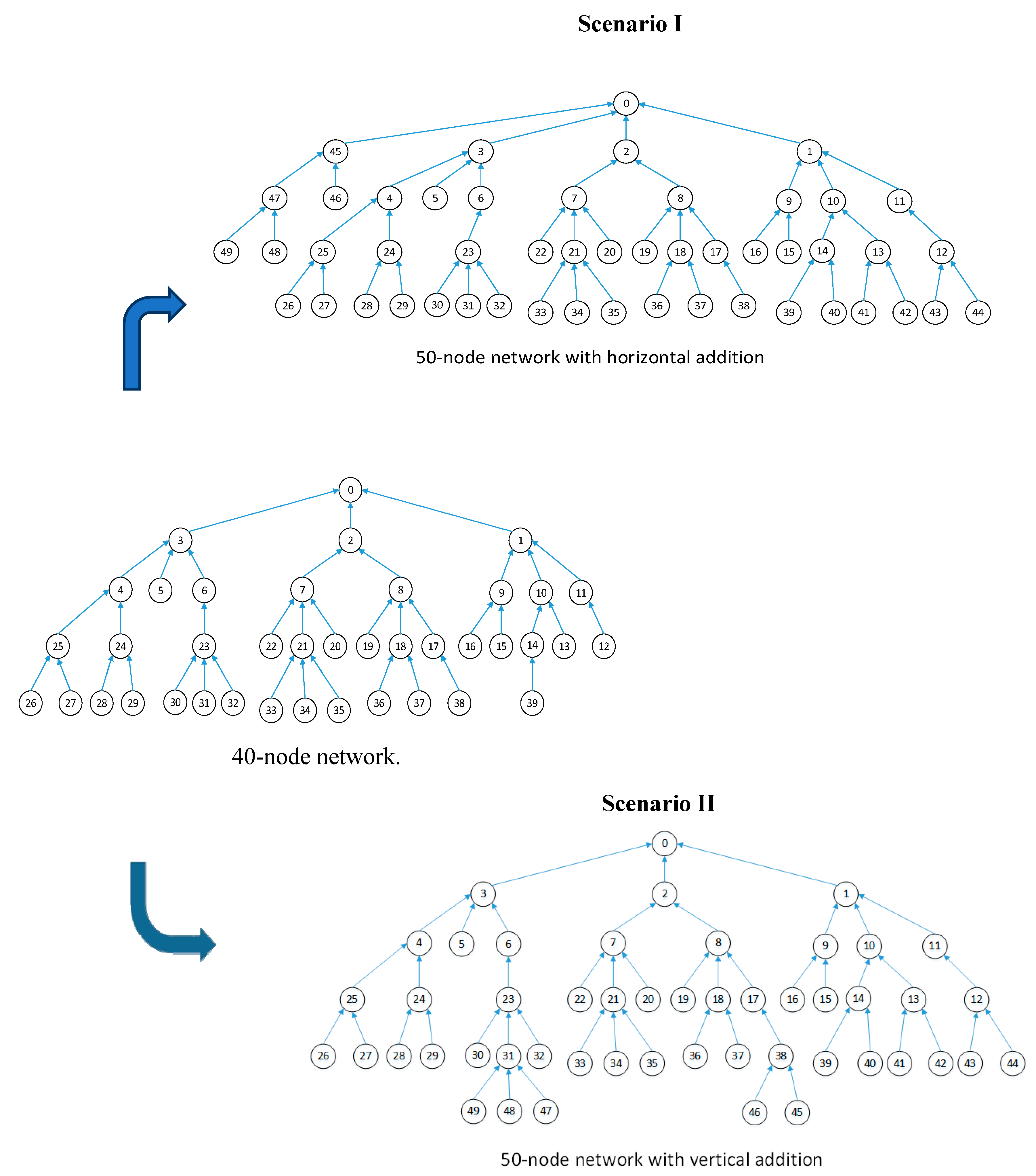
6.2. Experimental Scenarios

The experiment uses TLS-VaD as a tool to analyze the performance of the scheduling algorithms applied to network topologies that increase in dimension from 10 to 100 nodes, in increments of 10. In the meantime, starting from a network of 50 nodes, node addition is done in two ways, horizontal and vertical increments. With horizontal increments, network nodes are increased by adding children to the master node, whereas with vertical increments, network nodes are increased by adding new leaf nodes. The two types of node additions are illustrated in Figure 36.

Therefore, to get a performance comparison between IRByTSA, FTSA, and FLSA, the algorithms are applied to a network with two scenarios. In the first scenario, the scheduling algorithm is applied to a network that grows horizontally, and in the second scenario it is applied to a network that grows vertically. To collect all data at the master node, networks that increase in size vertically will require more cycles and timeslots than networks that increase horizontally. This happens because with vertical increase, the number of child nodes of the master node does not increase when the network dimensions increase, which will cause a bottleneck in the network. Thus, if a scheduling algorithm can show good performance in the second scenario, it indicates the reliability of the algorithm. In this test, we will see which of the scheduling algorithms (IRByTSA, FTSA, or FLSA) can produce the minimum number of active timeslots (λ), duty cycles (D), and cycles (C). The tests were performed using slotframe sizes of 200 timeslots.

6.3. Results and Discussion

TLS-VaD was used in the process of testing and retrieving data for performance comparison of IRByTSA, FTSA, and FLSA. The use of TLS-VaD eases the process. The TLS-VaD outputs are the data of active timeslots (λ), duty cycles (D), number of cycles (C), and total channel offsets (ChOffs) for IRByTSA, FTSA, and FLSA, collected in

Table 4. Active timeslot (λ) data of IRByTSA, FTSA, and FLSA.

Number of Nodes	IRByTSA		FTSA		FLSA
	Horiz.	Vert.	Horiz.	Vert.	Horiz.	Vert.
10	9	9	9	9	10	10
20	19	19	22	22	22	22
30	30	30	35	35	35	35
40	40	40	51	51	49	49
50	51	50	64	66	59	60
60	60	60	73	82	73	75
70	70	70	86	93	79	90
80	80	82	110	114	87	105
90	90	101	126	137	101	126
100	100	112	137	135	118	133

,

Table 5. Duty cycle (D) data of IRByTSA, FTSA, and FLSA.

Number of Nodes	IRByTSA		FTSA		FLSA
	Horiz.	Vert.	Horiz.	Vert.	Horiz.	Vert.
10	0.045	0.045	0.045	0.045	0.050	0.050
20	0.095	0.095	0.110	0.110	0.110	0.110
30	0.150	0.150	0.175	0.175	0.175	0.175
40	0.200	0.200	0.255	0.255	0.245	0.245
50	0.255	0.250	0.320	0.330	0.295	0.300
60	0.300	0.300	0.365	0.410	0.365	0.375
70	0.350	0.350	0.430	0.465	0.395	0.450
80	0.400	0.410	0.550	0.570	0.435	0.525
90	0.450	0.505	0.630	0.685	0.505	0.630
100	0.500	0.560	0.685	0.675	0.590	0.665

,

Table 6. Cycle (C) data of IRByTSA, FTSA, and FLSA.

Number of Nodes	IRByTSA		FTSA		FLSA
	Horiz.	Vert.	Horiz.	Vert.	Horiz.	Vert.
10	6	6	5	5	4	4
20	8	8	9	9	6	6
30	8	8	11	11	7	7
40	11	11	11	11	7	7
50	11	12	12	11	8	8
60	12	12	15	16	9	9
70	12	13	15	17	9	10
80	13	14	17	18	10	11
90	14	15	17	18	11	11
100	14	15	19	21	11	11

and

Table 7. Channel Offset (ChOff) data of IRByTSA, FTSA, and FLSA.

Number of Nodes	IRByTSA		FTSA		FLSA
	Horiz.	Vert.	Horiz.	Vert.	Horiz.	Vert.
10	12	12	11	11	9	9
20	26	26	27	27	21	21
30	40	40	45	45	31	31
40	62	62	62	62	43	43
50	78	80	78	79	56	59
60	95	97	101	113	67	76
70	110	122	116	148	81	90
80	131	143	144	184	97	107
90	152	159	167	204	112	117
100	169	175	192	233	124	135

. Furthermore, the data are displayed in graphical form to ease the process of performance comparison. As a reference for performance comparison, as stated in Section 4.2, the desired TSCH scheduling algorithm is one that can produce a minimum value of λ and minimum number of cycles (C).

Based on the λ data in Figure 37, with an increasing number of nodes, IRByTSA always produced a lower value of λ than FTSA (λ_FTSA) and FLSA (λ_FLSA). The value of λ in IRByTSA (λ_IRByTSA) remained the smallest when the network dimension increased. Only at the network dimension of 10 nodes was the value of λ_IRByTSA the same as λ_FTSA. However, this did not indicate anything significant, because the network dimension was still too small. The performance of the actual algorithm will only be seen on large networks, on which will arise more problems, such as processing time, processing delay, memory capacity, and so on. Efficient algorithms are mostly needed in large networks.

In addition to being the smallest, λ_IRByTSA also had a distance value that tended to get further away from λ_FTSA and λ_FLSA as network dimensions increased. This was indicated by the difference data between λ_IRByTSA and λ of FTSA and FLSA, as shown in

Table 8. Difference between λ_IRByTSA and λ of other algorithms.

Number of Nodes	(λIRByTSA − λFTSA)		(λIRByTSA − λFLSA)
	Horiz.	Vert.	Horiz.	Vert.
10	0	0	1	1
20	3	3	3	3
30	5	5	5	5
40	11	11	9	9
50	13	16	8	10
60	13	22	13	15
70	16	23	9	20
80	30	32	7	23
90	36	36	11	25
100	37	23	18	21

. In scenario I (Horiz.), the biggest difference between λ_IRByTSA and λ_FTSA was 37 timeslots, while between λ_IRByTSA and λ_FLSA the difference was 18 timeslots. In scenario II (Vert.), the biggest difference between λ_IRByTSA and λ_FTSA was 36 timeslots, while between λ_IRByTSA and λ_FLSA it was 25 timeslots.

In scenario II, the value of λ_IRByTSA was slightly increased, especially in network dimensions above 80 nodes. It is seen on the IRByTSA-Vert graph, which moved away from the IRByTSA-Horiz chart. However, in both scenarios I and II, λ_IRByTSA was always smaller than λ_FTSA and λ_FLSA. This indicates that IRByTSA had a high level of stability in the effort to get the best λ value and was superior to FTSA and FLSA in terms of its ability to reach the minimum λ value.

Meanwhile, for FTSA, its λ_FTSA value in scenario I and II was much greater than λ_IRByTSA. This shows the performance of FTSA in terms of getting a minimum value of λ, which was far below that of IRByTSA. The performance of FTSA, which was worse than IRByTSA, even though the way they work is most similar (Table 1 shows that all items are the same except for number 7), was evidence that the mechanism for providing transmission opportunities among child nodes based on turn was an important procedure to have a scheduling algorithm that can give minimum λ. As for FLSA, with increased network size, this algorithm performed better in producing λ values than FTSA but not better than IRByTSA. As seen in Figure 37, the value of λ_FLSA was always above λ_IRByTSA and almost always below FTSA, especially for networks with large dimensions.

Although λ_FTSA was far above λ_IRByTSA in both scenarios, the λ_FTSA values in scenarios I and II were not very different, whereas in FLSA, the values of λ_FLSA for scenarios I and II had quite large differences. IRByTSA also had the same tendency as FTSA, in that the λ_IRByTSA values for scenarios I and II were not much different. The difference in λ that was not large in scenarios I and II for IRByTSA and FTSA was evidence that the algorithm that gave transmission priority to higher-rank nodes would provide a stable λ value for various network conditions.

The value of λ would be directly proportional to the value of the duty cycle, as shown in Figure 38. The duty cycle generated by IRByTSA for the number of nodes ranging from 10 to 100 had the minimum value, which was below 0.5 for both scenarios. With a low duty cycle, the energy consumption of the nodes on the network will be low.

Figure 39 shows the number of cycles needed by each algorithm to collect all data in the master node. It can be seen that the number of cycles in IRByTSA (C_IRByTSA) was always smaller than the number of cycles in FTSA (C_FTSA), and this occurred in scenarios I and II. As the network size increased, the difference between the values of C_IRByTSA and C_FTSA became even greater. Based on these data, it was conclusive that in terms of speed in generating scheduling decisions, IRByTSA performed better than FTSA. IRByTSA required fewer cycles, because the process of providing transmission opportunities among child nodes was based on the turn. This highlights that it is important to apply procedure 7 in Table 1 to algorithms that give high priority to higher-rank nodes, such as IRByTSA and FTSA.

Meanwhile, in terms of the number of cycle parameters, FLSA shows the best performance, as indicated by the fewest cycles (C_FLSA) compared to C_IRByTSA and C_FTSA, for both scenarios I and II. This result is proof that link-scheduling algorithms with priority transmission from leaf nodes will produce scheduling decisions faster than algorithms prioritizing higher-rank nodes. The differences between C_FLSA, C_IRByTSA, and C_FTSA are shown in

Table 9. Difference between C_FLSA, C_IRByTSA, and C_FTSA.

Number of Nodes	|CFLSA − CIRByTSA|		|CFLSA − CFTSA|
	Horiz.	Vert.	Horiz.	Vert.
10	2	2	1	1
20	2	2	3	3
30	1	1	4	4
40	4	4	4	4
50	3	4	4	3
60	3	3	6	7
70	3	3	6	7
80	3	3	7	7
90	3	4	6	7
100	3	4	8	10

. The greatest difference between C_IRByTSA and C_FLSA lies in four cycles, while between C_FTSA and C_FLSA it is seven cycles, all of which occur in scenario II with a network dimension of 100 nodes. Based on this difference, the actual performance of IRByTSA in terms of the number of cycles is almost close to FLSA, because the difference between the two is only four cycles for network dimensions ranging from 10 to 100 nodes.

The performance of scheduling algorithms in terms of the need for channel offsets is presented in Figure 40. Through this figure we could compare the number of channel offsets required by each algorithm in the process of collecting all data at the master node. Meanwhile, the exact number of required channel offsets is presented in Table 7. The data show that IRByTSA usually requires fewer ChOffs than FTSA, especially in the same scenario and in large network dimensions. However, when compared to FLSA, IRByTSA needs more ChOffs. Figure 40 shows that with increased network size, the amount of ChOffs in IRByTSA was generally smaller than that in FTSA, but it was always greater than that in FLSA.

In fact, the more important thing to observe from ChOff data was ChOffs per cycle (ChOff/C), because ChOff/C will show the average number of ChOffs used in each cycle. As previously stated, according to the 802.15.4e standard, the number of available ChOffs is 16 channels. If there are more than 16, several transmissions will use the same channel offset, which can increase interference opportunities. Thus, the smaller the value of ChOff/C, the better, because it can reduce the possibility of interference. ChOff/C data are presented in

Table 10. ChOff/C data of scheduling algorithms.

Number of Nodes	IRByTSA		FTSA		FLSA
	Horiz.	Vert.	Horiz.	Vert.	Horiz	Vert.
10	2	2	2	2	2	2
20	3	3	3	3	4	4
30	5	5	4	4	4	4
40	6	6	6	6	6	6
50	7	7	7	7	7	7
60	8	8	7	7	7	8
70	9	9	8	9	9	9
80	10	10	8	10	10	10
90	11	11	10	11	10	11
100	12	12	10	11	11	12

, and based on the table, although these data for the scheduling algorithms varied in size, they show that the three algorithms had almost the same performance. The table shows that the value of ChOff/C for each scheduling algorithm was not much different in scenarios I and II. The performance of FTSA was usually below that of IRByTSA and FLSA, but based on ChOff/C, FTSA had the smallest ChOff/C value on a network dimension of 100 nodes for both scenario I and II. This shows that based on ChOff/C data, the three scheduling algorithms had relatively similar performance.

7. Conclusions

This research successfully developed a simulator that could be used as a tool to develop a centralized link-scheduling algorithm on the IEEE802.15.4e TSCH network. The developed simulator is known as the TSCH link-scheduling simulator, or TLS-VaD. As a research aid, the TLS-VaD provides the following facilities: (a) visualization for designed scheduling algorithms so that researchers can verify and validate them, (b) four types of data that can be used to analyze the performance of scheduling algorithms, and (c) a simplified experiment, because TLS-VaD can be used independently by researchers as a tool for processing and visualization scheduling data.

In the validity test, TLS-VaD was proven to be valid. This was indicated by a match between the visualization and output data generated by TLS-VaD with the link-schedule matrices generated by the scheduling algorithm. After passing the validity test, TLS-VaD was used to compare the performance of the Iman–Ramli bursty transmission scheduling algorithm (IRByTSA) with the first top scheduling algorithm (FTSA) and first leaf scheduling algorithm (FLSA). The parameters observed in this performance test were active timeslots (λ) and the speed of the algorithm in generating scheduling decisions.

The performance comparisons using TLS-VaD reveal that IRByTSA performed better than FLSA and FTSA, because it could save more power and generate scheduling decisions relatively quickly. The ability of IRByTSA to save power is shown by its λ value (λ_IRByTSA), which was smaller than the values in FTSA (λ_FTSA) and FLSA (λ_FLSA), while the ability to generate scheduling decisions in a relatively quick manner is shown by the number of cycles (C) required by IRByTSA (C_IRByTSA), which was smaller than C in FTSA (C_FTSA) and almost close to that in FLSA (C_FTSA). Although in terms of the number of cycles IRByTSA was not able to show the best performance, the difference between C_IRByTSA and C_FLSA, only four cycles, could be compensated by the difference between λ_IRByTSA and λ_FLSA, which amounted to 25 timeslots.

The performance comparison of these three scheduling algorithms was in line with the hypotheses. This was reinforced by two additional pieces of information: the performance of the three algorithms was almost the same in terms of the ChOff/C parameter, and the C_IRByTSA value was almost close to C_FLSA. This research proved that TLS-VaD could be used as a tool to develop a centralized link-scheduling algorithm on the IEEE802.15.4e TSCH network.

References

1. Atzori, L.; Iera, A.; Morabito, G. Understanding the Internet of Things: Definition, potentials, and societal role of a fast evolving paradigm. Ad Hoc Netw. 2017, 56, 122–140. [Google Scholar] [CrossRef]
2. Li, S.; Da Xu, L.; Zhao, S. The internet of things: A survey. Inf. Syst. Front. 2015, 17, 243–259. [Google Scholar] [CrossRef]
3. Bizanis, N.; Kuipers, F.A. SDN and virtualization solutions for the Internet of Things: A survey. IEEE Access 2016, 4, 5591–5606. [Google Scholar] [CrossRef]
4. Chen, Y.; Han, F.; Yang, Y.H.; Ma, H.; Han, Y.; Jiang, C.; Lai, H.-Q.; Claffey, D.; Liu, K.R. Time-reversal wireless paradigm for green Internet of Things: An overview. IEEE Internet Things J. 2014, 1, 81–98. [Google Scholar] [CrossRef]
5. Palattella, M.R.; Thubert, P.; Vilajosana, X.; Watteyne, T.; Wang, Q.; Engel, T. 6tisch wireless industrial networks: Determinism meets ipv6. In Internet of Things; Springer: Cham, Switzerland, 2014; pp. 111–141. [Google Scholar]
6. Thubert, P.; Palattella, M.R.; Engel, T. 6TiSCH centralized scheduling: When SDN meet IoT. In Proceedings of the 2015 IEEE Conference onStandards for Communications and Networking (CSCN), Tokyo, Japan, 28–30 October 2015; pp. 42–47. [Google Scholar]
7. Bera, S.; Misra, S.; Vasilakos, A.V. Software-defined networking for internet of things: A survey. IEEE Internet Things J. 2017, 4, 1994–2008. [Google Scholar] [CrossRef]
8. Thubert, P. An Architecture for IPv6 over the TSCH mode of IEEE 802.15. 4. Working Draft. Available online: https://tools.ietf.org/id/draft-ietf-6tisch-architecture-15.html (accessed on 14 December 2019).
9. Palattella, M.R.; Accettura, N.; Grieco, L.A.; Boggia, G.; Dohler, M.; Engel, T. On optimal scheduling in duty-cycled industrial IoT applications using IEEE802. 15.4 e TSCH. IEEE Sens. J. 2013, 13, 3655–3666. [Google Scholar] [CrossRef]
10. Palattella, M.R.; Accettura, N.; Dohler, M.; Grieco, L.A.; Boggia, G. Traffic aware scheduling algorithm for reliable low-power multi-hop IEEE 802.15. 4e networks. In Proceedings of the 2012 IEEE 23rd International Symposium on Personal Indoor and Mobile Radio Communications (PIMRC), Sydney, Australia, 9–12 September 2012; pp. 327–332. [Google Scholar]
11. Palattella, M.R.; Accettura, N.; Dohler, M.; Grieco, L.A.; Boggia, G. Traffic-aware time-critical scheduling in heavily duty-cycled IEEE 802.15. 4e for an industrial IoT. Proc. IEEE Sens. 2012, 2012, 1–4. [Google Scholar]
12. Santoso, I.H.; Ramli, K. IRByTSA: A Novel link-scheduling algorithm for IEEE802.15.4e TSCH Network. J. Theor. Appl. Inf. Technol. 2019, 97, 2725–2738. [Google Scholar] [CrossRef]
13. Santoso, I.H.; Ramli, K. Speed improvement of centralized scheduling algorithm on IEEE 802.15. 4e TSCH netwok using heuristic method. J. Commun. 2017, 12, 661–667. [Google Scholar] [CrossRef]
14. Meng, M.; Yujun, Z.; Dadong, Z.; Fan, C. Scheduling for Data Transmission in Multi-Hop IEEE 802.15. 4e TSCH Networks. Mob. Netw. Appl. 2018, 23, 119–125. [Google Scholar] [CrossRef]
15. Ojo, M.; Giordano, S.; Portaluri, G.; Adami, D.; Pagano, M. An energy efficient centralized scheduling scheme in TSCH networks. In Proceedings of the 2017 IEEE International Conference on Communications Workshops (ICC Workshops), Paris, France, 21–25 May 2017; pp. 570–575. [Google Scholar]
16. Chen, T.S.; Kuo, S.Y.; Kuo, C.H. Scheduling for data collection in multi-hop IEEE 802.15. 4e TSCH networks. In Proceedings of the 2016 International Conference on Networking and Network Applications (NaNA), Hakodate, Japan, 23–25 July 2016; pp. 218–222. [Google Scholar]
17. Choi, K.H.; Chung, S.H. A new centralized link scheduling for 6TiSCH wireless industrial networks. In Internet of Things, Smart Spaces, and Next Generation Networks and Systems; Springer: Cham, Switzerland, 2016; pp. 360–371. [Google Scholar]
18. Livolant, E.; Minet, P.; Watteyne, T. The cost of installing a 6tisch schedule. In International Conference on Ad-Hoc Networks and Wireless; Springer: Cham, Switzerland, 2016; pp. 17–31. [Google Scholar]
19. Shreedhar, M.; Varghese, G. Efficient fair queuing using deficit round-robin. IEEE/ACM Trans. Netw. 1996, 3, 375–385. [Google Scholar] [CrossRef]
20. Sayenko, A.; Alanen, O.; Karhula, J.; Hämäläinen, T. Ensuring the QoS requirements in 802.16 scheduling. In Proceedings of the 9th ACM International Symposium on Modeling Analysis and Simulation of Wireless and Mobile Systems, Torremolinos, Spain, 2–6 October 2006; pp. 108–117. [Google Scholar]
21. Khoufi, I.; Minet, P.; Livolant, E.; Rmili, B. Building an IEEE 802.15. 4e TSCH network. In Proceedings of the 2016 IEEE 35th International Performance Computing and Communications Conference (IPCCC), Las Vegas, NV, USA, 9–11 December 2016; pp. 1–2. [Google Scholar]
22. Felicetti, L.; Femminella, M.; Reali, G. A simulation tool for nanoscale biological networks. Nano Commun. Netw. 2012, 3, 2–18. [Google Scholar] [CrossRef]
23. Beshay, J.D.; Subramani, K.S.; Mahabeleshwar, N.; Nourbakhsh, E.; McMillin, B.; Banerjee, B.; Prakash, R.; Du, Y.; Huang, P.; Xi, T.; et al. Wireless networking testbed and emulator (winetester). Comput. Commun. 2016, 73, 99–107. [Google Scholar] [CrossRef] [Green Version]
24. De Guglielmo, D.; Brienza, S.; Anastasi, G. IEEE 802.15. 4e: A survey. Comput. Commun. 2016, 88, 1–24. [Google Scholar] [CrossRef]
25. Zheng, J.; Lee, M.J. A Comprehensive Performance Study of IEEE 802.15.4. Sens. Netw. Oper. 2004, pp. 218–237. Available online: https://sites.google.com/site/jzhengresearch/papers/paper1_wpan_performance.pdf (accessed on 17 December 2019).
26. 802.15.4e-2012: IEEE Standard for Local and Metropolitan Area Networks—Part 15.4: Low-Rate Wireless Personal Area Networks (LRWPANs) Amendment 1: MAC Sublayer; Institute of Electrical and Electronics Engineers Std. IEEE Computer Society: New York, NY, USA, 2012.
27. Palattella, M.R.; Accettura, N.; Vilajosana, X.; Watteyne, T.; Grieco, L.A.; Boggia, G.; Dohler, M. Standardized protocol stack for the internet of (important) things. IEEE Commun. Surv. Tutor 2013, 15, 1389–1406. [Google Scholar] [CrossRef] [Green Version]
28. Watteyne, T.; Palattella, M.R.; Grieco, L. Using IEEE 802.15. 4e Time-Slotted Channel Hopping (TSCH) in the Internet of Things (IoT): Problem Statement. Available online: https://tools.ietf.org/html/rfc7554 (accessed on 14 December 2019).
29. NS3. Current Development. 7 July 2019. Available online: https://www.nsnam.org/wiki/Current_Development (accessed on 3 November 2018).
30. Atlassian Inc. The 6TiSCH Simulator. Available online: https://bitbucket.org/6tisch/simulator (accessed on 16 April 2019).
Figure 1. 6TiSCH protocol stack. 6TiSCH, Internet protocol version 6 (IPv6) over the time synchronized channel hopping (TSCH) mode of IEEE802.15.4e.
Electronics 08 01555 g001
Figure 2. Superframe structure of IEEE802.15.4. CAP, contention access period; CFP, contention free period; and GTS, guaranteed timeslot.
Electronics 08 01555 g002
Figure 3. TSCH slotframe with six timeslots.
Electronics 08 01555 g003
Figure 4. Timeslot channel hopping mechanism in the IEEE802.15.4e standard.
Electronics 08 01555 g004
Figure 5. (a) TSCH network with tree topology and (b) example of link schedule for data collection.
Electronics 08 01555 g005
Figure 6. Transmit, receive, idle, and data collection processes.
Electronics 08 01555 g006
Figure 7. Graph G = (V, E) modeling a network with tree topology.
Electronics 08 01555 g007
Figure 8. Two types of links on TSCH networks: (a) duplex conflict links (DCLs) and (b) duplex conflict free links (DCFLs).
Electronics 08 01555 g008
Figure 9. Network topology of 16 nodes.
Electronics 08 01555 g009
Figure 10. The flowchart of IRByTSA.
Electronics 08 01555 g010
Figure 11. Flowchart of program start and variable initialization of IRByTSA.
Electronics 08 01555 g011
Figure 12. Flowchart of the L1 loop in IRByTSA.
Electronics 08 01555 g012
Figure 13. Flowchart of the L2 loop in IRByTSA.
Electronics 08 01555 g013
Figure 14. Decision-making process to give a turn to a node in IRByTSA.
Electronics 08 01555 g014
Figure 15. Process of checking number of child nodes in IRByTSA.
Electronics 08 01555 g015
Figure 16. Giving a turn to a child node (parent node with more than one child).
Electronics 08 01555 g016
Figure 17. Giving turns to child nodes (parents with more than one child and qz = 0).
Electronics 08 01555 g017
Figure 18. Process of giving a turn to a child node (parent has only one child node and qz > 0).
Electronics 08 01555 g018
Figure 19. Process for determining TS (s) in IRByTSA.
Electronics 08 01555 g019
Figure 20. Application of IRByTSA on 16-node networks.
Electronics 08 01555 g020
Figure 21. FTSA.
Electronics 08 01555 g021
Figure 22. FTSA application on 16-node networks.
Electronics 08 01555 g022
Figure 23. FLSA.
Electronics 08 01555 g023
Figure 24. Network scheduling using FLSA.
Electronics 08 01555 g024
Figure 25. Flowchart of how the TSCH link-scheduling visualization and data processing (TLS-VaD) works.
Electronics 08 01555 g025
Figure 26. Use case diagram.
Electronics 08 01555 g026
Figure 27. The activity diagram of the simulation feature.
Electronics 08 01555 g027
Figure 28. The activity diagram of the experiment feature.
Electronics 08 01555 g028
Figure 29. Network topology and its adjacency matrix.
Electronics 08 01555 g029
Figure 30. Scheduling matrices as an output.
Electronics 08 01555 g030
Figure 31. The flowchart of TLS-VaD.
Electronics 08 01555 g031
Figure 32. Menus and input systems in TLS-VaD.
Electronics 08 01555 g032
Figure 33. Transmit and receive visualization on the simulation menu.
Electronics 08 01555 g033
Figure 34. Experiment section in the TLS simulator.
Electronics 08 01555 g034
Figure 35. Result table in the experiment menu.
Electronics 08 01555 g035
Figure 36. Scenarios I and II in algorithm testing using TLS-VaD.
Electronics 08 01555 g036
Figure 37. Value of λ in IRByTSA, FTSA, and FLSA.
Electronics 08 01555 g037
Figure 38. Duty cycles of IRByTSA, FTSA, and FLSA.
Electronics 08 01555 g038
Figure 39. Number of cycles in IRByTSA, FTSA, and FLSA.
Electronics 08 01555 g039
Figure 40. Total required channel offset of IRByTSA, FTSA, and FLSA.
Electronics 08 01555 g040