Abstract
Predictive current control (PCC) applied on permanent magnet synchronous motors (PMSMs) has been developed into mainly three methods: the conventional finite-control-set PCC, the double voltage vectors PCC, and deadbeat PCC. However, each approach has its particular calculation way for voltage vectors selection and respective execution duration. This paper, based on the deadbeat idea, presents a unified predictive current control scheme of PMSMs. Under this scheme, the prior three classes are able to be clearly unified into one frame with lower calculation effort. Furthermore, to cope with problem of parameter mismatch in dq-axis current predictive model, a integrated identification method is proposed. Firstly, data selectors are designed to reject abnormal data of sampling signals, and then the interval-varying multi-innovation least squares algorithm is combined with forgetting factor (V-FF-MILS) to approximate the error terms caused by electromagnetic parameters error. The estimated results are online fed to the model of PMSM to enhance its accuracy. Finally, the processor in loop (PIL) simulation results verify that the proposed integrated scheme has advantages in current control of PMSMs with large-scale parameter uncertainty.
1. Introduction
Owing to its advantages on efficiency, power density, and compact structure, PMSMs have been widely employed in various electrical drive appliances in vehicle, aerospace, and other industrial fields. There are a variety of control strategies designed to improve PMSMs’ output performance. Field-oriented control (FOC), also called vector control, and direct torque control (DTC) are the two most common control frames together with many other modified methods. It is well known that FOC and DTC have limitations on necessity of independent d-q current controllers with a pulse modulator and considerable torque ripple, respectively []. Recently, thanks to the continuous advancement of digital signal processing technology over the last decades [], the model predictive control (MPC), with intuitive operation principle and good transient performance, has gained attention on regulating the output current or torque of PMSMs, yielding the predictive current control (PCC). Overall, the PCC can be divided into three categories: the conventional finite-control-set PCC, the Double VVs, and deadbeat PCC. They have been successfully implemented on controllers of PMSMs [,].
The conventional finite-control-set PCC, also known as direct PCC, takes advantage of the inherent nature of inverter that has a finite number of switching states S, where for the commonly used two-level voltage source inverter; thus, there are eight voltage vectors (VVs) including six active VVs and two null VVs. All the VVs are used to predict possible stator currents based on the discrete model of motor. The one that minimizes a cost function evaluating the error between the reference current i and the predictions and other constraints is selected as the action of the next control period. Although the conventional PCC has feature of intuitive principle, there are several drawbacks, e.g. high current ripple as amplitude, phase of the action VV cannot be adjusted, and computational burden result from the enumerated way to search the optimal VV. The inverter is operated in a variable switching frequency because of only one VV per period with no need for a modulator, causing large harmonics []. To overcome this, the Double VVs PCC is introduced by taking account of exerting two voltage vectors using a PWM modulator in a control period. Combination forms of two VVs have been explored. The authors of [,,] considered one active vector and a successively null vector as a set, thus amplitude of the resultant vector can be adjusted. However, Zhang and Yang [] showed it has an inferior steady-state performance at high speed. Therefore, Liu et al. [] considered all the feasible combinations of two VVs so that the phase of the composed vector can be adjusted, but the situation that two non-adjacent vectors are combined would increase the switching loss of inverter. The duty cycle of each vector is calculated based on the current dead-bead principle in the above methods, which considers the current will reach the reference value at the end of this operation.
The Deadbeat PCC is similar to the FOC scheme, which usually has a space vector PWM modulator, and its optimal control set composed by two adjacent active VVs and a null VV is determined by the reference voltage, which is directly obtained from the predictive model of PMSMs based on the deadbeat idea [], while that of FOC is from a specific PI or other complex current controller.
The performance differences about the three PCC schemes can be found in []. Each scheme has its unique advantage, such as less nonlinearity of inverter introduced for direct PCC in each control period. In this paper, the above three methods are simply denoted as 1-PCC, 2-PCC and 3-PCC, respectively. The numeric symbols represent the number of voltage vectors applied per control period. Currently, there are numerous variations of those schemes implemented in different computation ways. For example, the 1-PCC is implemented on -frame based on an enumerated way, while the 2-PCC usually takes d-q coordinate, which is not convenient for engineers. One study on unifying the 1-PCC and 2-PCC method in one frame [] reveals that an alternative cost function about voltage vector is equivalent to the conventional one, but its calculation process is still not intuitive. This paper proposes a generalized predictive current control scheme based on the principle of deadbeat control and vector composition in an explicit way. It is shown that 3-PCC can easily be reduced to 2-PCC and 1-PCC by judging simple linear equations. The durations of VVs for 2-PCC can be calculated simultaneously. Consideration for the system uncertainty can also be included.
An inevitable issue is that the PCC heavily relies on the model parameters of motor, resulting in current tracking performance deterioration when occurring in parameter mismatch. The nonlinear control is widely used to cope with this situation. For example, the sliding mode observers are frequently designed to estimate the disturbance caused by parameter uncertainty [,,]. The uncertain term in the predictive model can be replaced by nonlinear function []. Advanced robust techniques are often introduced to design control law, such as the control-Lyapunov function [], disturbance estimation [], and differential flatness []. Another strategy lies in the parameter identification, such as a recursive inductance estimator [], multi-parameter identification with a decoupling method [], model reference adaptive technique [], extended Kalman filter [], modified particle swarm optimization [], Adaline neural network [], etc. All those methods aim to acquire accurate parameters, which is not necessary in the PCC schemes. In this paper, we estimate three model error terms caused by parameter perturbation. Thus, the identification model can be simplified into a linear regression model. Then, a integrated identification method is proposed to approximate the error terms.
This paper is organized as follows. The predictive model of a surface-mounted PMSM and the calculation of the inverter’s output voltage are presented in Section 2. Section 3 proposes the generalized predictive current control scheme. The model identifying method based on a modified multi-innovation recursive least square to estimate the model error is presented in Section 4. Section 5 presents the PIL test results of proposed method. Finally, the conclusions are drawn in Section 6.
2. System Model
2.1. Discrete Predictive Model of PMSMs
The stator voltage equation of a surface-mounted PMSM described in the synchronous reference can be found in []. After discretizing it by Euler forward difference method, the current predictive model in dq frame can be expressed as follows,
where , , , and
is the predictive current at instant with respect to the control input , is the sampling current at instant k and the electrical angular velocity , and represents the sample period of current. The matrices of nominal model , , and are determined by the values of , , and , which represent the electromagnetic parameters, with stator resistance, inductance, and magnetic flux, respectively. , , and are the perturbation parts composed of three error terms independently, which result from differences between nominal parameters and real values. For instance, the estimation errors of stator resistance and inductance jointly lead to the error term . The symbol diag(.) means it is a diagonal matrix. The control input is produced by a switching sequence of inverter per control period, thus and are mean voltages at the d-axis and q-axis, respectively.
2.2. Inverter Model
As shown in Figure 1, the PMSM is fed by a two-level voltage source inverter, which is composed of three phase legs (), and each leg has two opposite switching states. Since there are eight different switching sates, which can be defined as , n = 0, …, 7, the index number satisfies , and each one generates a voltage vector . The stator voltage in -axis can be expressed as a function of the switching states
where
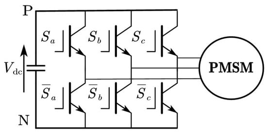
Figure 1.
PMSM fed by a two-level voltage source inverter.
is the DC bus voltage of inverter and represents electrical angular of rotor at instant k. The transformation method is based on the amplitude unchanged principle, thus the coefficient is . It would be if the power unchanged principle were adopted. Obviously, when n equals 0 or 7, .
After gaining stator voltage, the control input can be obtained under the principle of volt-second balance
where . , , and are durations of the respective stator voltage vector during the kth control period. is zero vector, thus
where the is duty cycle vector of active voltage vectors and . We define ; combined with Equation (2), can be expressed as
3. The Proposed Control Scheme
The conventional one-horizon PCC method has a time delay between the measurements and actuation, which causes current ripple []. A simple solution to compensate this delay is to consider a two-step-ahead prediction. The predictive current at instant can be obtained by
The angular velocity is deemed as a constant during the two sampling periods. Because current dynamics are much faster than those of speed, . The control aim is achieved by a cost function that is defined as follows:
where , as the output of speed controller, is the reference current that is also deemed as a constant from kth to (k + 2)th period. In this paper, we take the Euler 2-norm to define the cost function, thus the objective is to search the control action to minimize the distance of between reference current and predictive value.
3.1. Deadbeat PCC
The reference stator voltage in -frame is obtained based on deadbeat principle and the inverse model of PMSM, which is shown as follows:
The matrix is obviously invertible. We can define an alternative cost function with respect to motor voltage
It is easily seen that, if the control input gradually approximates the reference voltage , the resultant current will approach the reference current . Therefore, the cost function is equivalent to . After obtaining the reference voltage, we need to make sure its position in the voltage vector plane that is divided into six sectors, as shown in Figure 2. The sector position of reference voltage can be calculated by solving an arc-tangent function
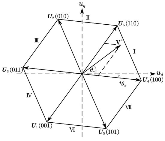
Figure 2.
Position of reference voltage in space voltage vector plane.
The reference voltage is composed of the two active voltage vector
where the and are two adjacent vectors, and to flexibility produce pulse sequence; for example, when the reference voltage is located in Sector , then . Clearly, is invertible, thus the duty cycles of the vectors are calculated by
where , which can be calculated offline to reduce the computational burden. N denotes the sector index. can be directly obtained from the elements of the park transformation matrix . If , it means the reference voltage has gone over the scope of voltage vector plane, and a common overmodulation method can be used . The duty cycle of the null VV is calculated by , and then a space vector pulse width modulation (SVPWM) is applied to produce the switching sequence of inverter.
3.2. Direct PCC
The direct PCC selects only one optimal voltage vector that minimizes the cost function in Equation (10), which aims to search error voltage vector with shortest length. After locating position of reference voltage, the two adjacent active VV and null VV in the sector are feasible optimal VV and necessary to be checked by the cost function. For example, we assume reference voltage is located in Sector , as shown in Figure 3a. The triangular sectors are divided into three equal parts by their three center lines. The reference voltage is located in the third part. The shortest is the result of the difference between and active voltage vector , which is depicted by the red dashed line. As a result, is selected as the optimal VV. Similarly, if reference VV lies in the first part or second part of Sector , then the optimal VV is or , respectively. Therefore, once we confirm to which part the reference voltage belongs, the optimal actuation can be directly obtained. The three parts in a sector are mapped in the coordinate axis because of the linear feature of vector synthesis. As shown in Figure 3b, each part can be judged by a set of inequalities as follows.
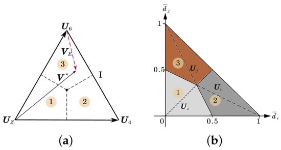
Figure 3.
Selection of optimal VV: (a)Distribution of reference voltage, (b) Confirm the optimal VV.
Consequently, after getting and with Equation (13), we can directly select the optimal VV from in the above inequalities of duty cycles, which greatly reduce the computational burden compared with the enumeration-based method, and makes it convenient to switch control method from Deadbeat PCC to Direct PCC.
3.3. Double VVs PCC
This method needs to apply two VVs in every control period, which can either be one active VV and one null VV or two active VVs, and the resultant voltage vector is located on one side of a triangular sector. Thus, the exploration to find the minimum cost function is to identify the shortest distance between the reference VV and the near sides. Obviously, needs to be perpendicular to the nearest side. For instance, as depicted in Figure 4a, the reference voltage is located in the second part, thus it is close to . is normal to and obtained by
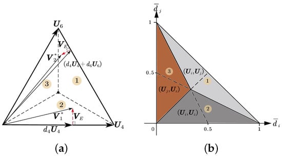
Figure 4.
Selection of optimal VVs: (a) The shortest error VV, (b) Confirm the optimal VVs.
It is noted that is in the same direction as vector , thus
is the actual duty cycle, the residual duration belongs to the null voltage vector , and the principle to choose a null VV is subject to minimum switching number. Similarly, when reference voltage lies in the first part in Figure 4a, the optimal vector combination is (). equals , which is in the same direction as vector , and . Thus, the duration of can be calculated as follows:
In summary, we firstly need to identify in which part the reference voltage is located, and then confirm the optimal vector combination. Finally, we calculate the respective duty cycle. The process is summarized as below:
Supplementing other sectors in the voltage vector plane, we can acquire the maps to directly select optimal actuation according to the position of reference voltage. Figure 5a shows the distribution of optimal voltage vector of direct PCC method, and its duration is the whole control period with no need for a pulse modulator. The distribution of optimal two VVs combination is shown in Figure 5b. The execution time of two VVs is ; thus, a pulse modulator is needed to produce switching signals. It can be seen that the above three PCCs are unified into a frame with little calculation effort, and we can easily adjust the current control method in practical application.
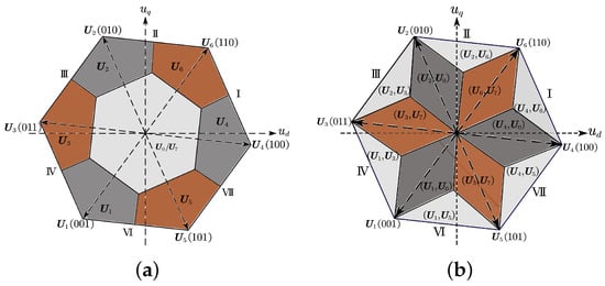
Figure 5.
Distribution of optimal VVs: (a) Optimal VV of Direct PCC, (b) Optimal VVs of Double VVs PCC.
Inevitably, predictive current control heavily depends on the accuracy of motor model, and an exact predictive model is the precondition of this control scheme. Therefore, an identification algorithm aiming to approximate the uncertain terms in model is incorporated into the scheme. A block diagram of the unified predictive current control (UPCC) scheme is depicted in Figure 6. Before acquiring accurate model, 1-PCC is chosen to be the operation method because of its better robustness performance [], and the fewer switches also reduce the influence of dead band of inverter per period. The results of identification are fed into the PMSM’s model online, thus enhancing the model accuracy. The detailed estimation method is introduced in the next section.
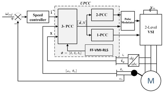
Figure 6.
The proposed control scheme.
4. Identification for Model Uncertain Term
In this section, we estimate the three error terms caused by inaccurate resistance, inductance, and flux linkage in the current error predictive model, rather than identify the electromagnetic parameter in the nonlinear model. Based on Equation (1), we can predict the ()th current at the kth instant, and acquire the real value at the next instant of the predictive current error model , namely
It can be seen that we can estimate the whole error vector just by the q-axis error equation. Since the sample time of angular velocity is much slower than electrical dynamic, staying constant during several sampling intervals of current is not accurate if only the q-axis dynamic information is used. Therefore, we firstly utilize the d-axis electrical information to identify the first two error term and , and then independently analyze the third term .
Most of identification methods make full use of the dynamic information of motor system, but the obtained current and rotor position of the system is commonly accompanied by large noise signal, which causes failure of some ideal methods despite the presence of the filter. An effective method of interval-varying multi-innovation least squares (V-MILS) was proposed by Ding et al. [] to overcome missing measurement data. Thus, we combine a data selector and interval-varying multi-innovation least squares with forgetting factor (V-FF-MILS) algorithm to identify the error vector in d-axis prediction error equation.
Firstly, we define an integer sequence , s=0, 1, 2…to label the signals passed from selector as
satisfies , and the interval . and are the reasonable ranges of d-axis current and its predictive error, respectively. Based on the principle of V-MILS, the predictive error model of d-axis current can be represented in linear regressive form,
where
The interval-varying multi-innovation least squares with forgetting factor algorithm can be written as follows,
The forgetting factor satisfies . The initial condition is set as . The two error terms are approximated after finite recursive estimation. A termination principle of identification is designed as
and are the maximum and minimum value of identification during an interval with enough length. can reflect the fluctuation amplitude of online identifying results. After acquiring estimated and , the third error term can be derived by real-time information of q-axis current equation. Our strategy is to command the angular velocity of rotor in a constant values; choose the effective q-axis data by a similar selector ;, and then online analyze the proportional relation between the error term result from and in a linear regression technique. The ratio is the estimated value of .
5. PIL Test Results
The proposed methods were verified using processor-in-loop (PIL) simulation, which means the algorithm was conducted in a real microprocessor. The mathematical model of the plant was run in the PC host and exchanged data by serial communication. The real parameters of this PMSM were , mH, Wb, and . The DC bus voltage was V. The speed controller utilized PI regulator with and . Its sample time was set equal to 1 ms, and for current controller was 100 s. The TI TMS32F28335 was selected as control processor. The identification for three uncertain term in motor model was tested in two designed cases. In Case 1, the nominal resistance was enlarged two times, with three times flux linkage, and the inductance was a quarter of real values. In Case 2, we assumed that inductance was known but a small deviation was artificially created to generate enough current prediction error. The nominal resistance and flux linkage were enlarged as and , independently. Both cases considered the disturbance of noise signal. All the sampling signals were accompanied with a noise signal of which expectation equaled zero, and variance was . Results are presented and compared in the following figures. The labels 1-PCC, 2-PCC, and 3-PCC represent the proposed predictive current control methods. C-PCC, FOC, and DTC-SVM denote the conventional PCC, vector control, and direct torque control with a space vector modulator, respectively.
Figure 7a and Figure 8 show the transient performances at the start-up phase after the speed command of 1000 r/min. It is illustrated that all methods have the same current transient response in Figure 7a,b, in which both approximate current reference value at the time of 0.005 s. In Figure 8, performance of speed response at start-up phase of all methods are compared. They all show a similar capability that reaches the speed command at about 0.2 s, which verifies that the proposed PCCs keep the superior transient performance of classical current regulation strategies.
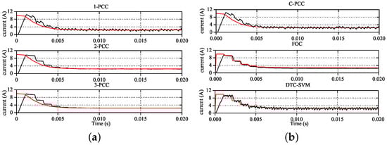
Figure 7.
q-axis current response at start-up: (a) Performance of proposed PCCs, (b) Performance of comparison group.
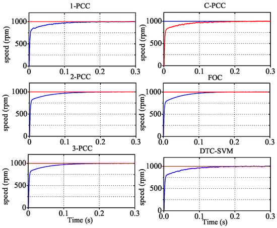
Figure 8.
Speed response comparison at start-up.
In Figure 9 and Figure 10, the transient performance of the proposed controller is further verified under the change of load and speed. Figure 9 compares the q-axis current tracking capability, where the red line denotes the reference values from speed controller, it can be seen that C-PCC and 1-PCC have almost the same current response when the load is suddenly changed from 0.2 Nm to 0.4 Nm at the instant of 0.5 s. Performance of 3-PCC is close to that of FOC, which are both slightly better than 2-PCC with less ripple during tracking the reference current. DTC-SVM has the largest ripple during the transient process. In Figure 10, we gradually reduce the rotational speed from 1000 r/min to −1000 r/min at a constant rate within 1 s. The u-phase current regulation capabilities of 1-PCC and C-PCC show same tracking accuracy, but they both encounter large current perturbation when the motor is in counter rotation at the time of 4.0 s. 2-PCC, 3-PCC, and FOC show higher accuracy whether tracking phase current or speed. Similarly, DTC-SVM presents large ripple of u-phase current with the speed adjusted.
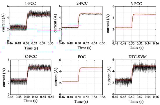
Figure 9.
q-axis current tracking when occurring load perturbation.
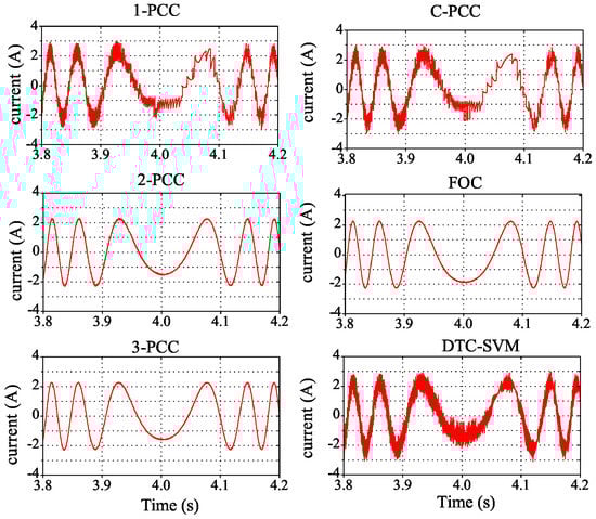
Figure 10.
u-phase current response comparison when speed adjusted.
Figure 11a,b compares the steady-state performance of output torque within 0.1 s, and the standard deviations of q-axis current that represent the degree of torque ripple are 0.3689 and 0.3687 for C-PCC and 1-PCC, respectively, both inevitably leading to large output torque ripple. Relatively, the steady-state errors in 2-PCC and 3-PCC are much smaller, with 0.0576 and 0.0181 standard differences, respectively. These results are in accordance with other researcher’s work []. FOC shows a high accuracy for torque, while DTC-SVM is the worst case. It is noted that the control parameters of FOC in this test were searched by optimization algorithm in Matlab software to make sure of the best output performance.
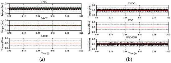
Figure 11.
Output torque in steady-state: (a) Performance of proposed PCCs, (b) Performance of comparison group.
In Figure 12, the left column depicts total harmonic distortion (THD) of u-phase current of the proposed PCCs in steady state, with 20.05%, 5.84%, and 1.28% for 1-PCC, 2-PCC, and 3-PCC, respectively. The right column presents the corresponding THD of comparison group. Obviously, the optimal FOC has minimum THD, which is roughly equal to that of 3-PCC. The largest THD belongd to DTC-SVM. The harmonic quality of C-PCC and 1-PCC are similar based on the same current response and THD values. Therefore, the results in Figure 11a,b and Figure 12 show that the proposed approaches have advantage in steady-state output accuracy, especially 2-PCC and 3-PCC.
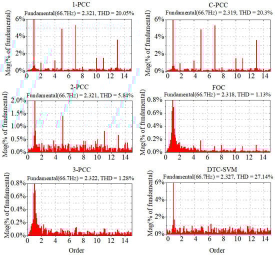
Figure 12.
Harmonic quality comparison.
The quantifiable metrics in speed response time in start-up phase and the steady performance verified by harmonic component and current standard deviation of each approach are listed in Table 1. It can be seen that the transient response has no obvious difference. 2-PCC and 3-PCC present superior steady output accuracy. Although FOC has slightly better performance, it is difficult to obtain the optimal control parameters in practical application, while the proposed PCCs have no need of parameter tuning.

Table 1.
Quantifiable metrics comparison.
The execution duration of PCC has important influence on its output capability. The conventional predictive current controller is based on an enumerated search strategy causing a high computation time. As shown in Figure 13, the execution time of C-PCC is 88.7 s, followed by 62.8 s for 2-PCC and 60.8 s for 3-PCC. 1-PCC takes the minimum computing time as it does not include the pulse modulator comparing with 2-PCC and 3-PCC. Therefore, the proposed calculation frame has advantage in alleviating computational burden.
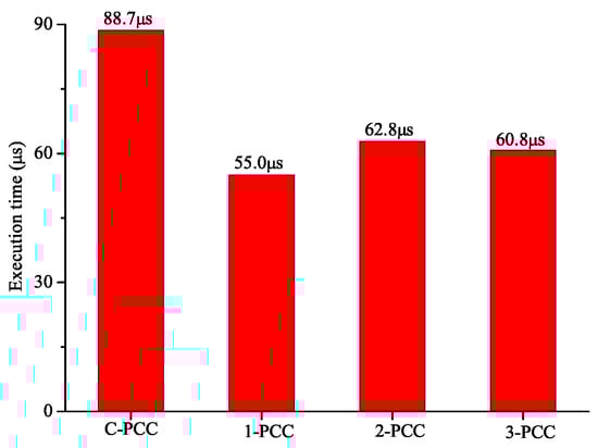
Figure 13.
Execution time for each algorithm.
Figure 14a,b, Figure 15a,b, Figure 16a,b, Figure 17a,b and Figure 18a,b show the performance of the proposed integrated identification algorithm. Estimated values of and are shown in Figure 14a,b, respectively. It can be seen that both estimated values in ideal environment have high steady-state accuracy of less than 5% error rates under the wave rate . However, when they are faced with noise condition, the results show small fluctuation and slight deviation from the actual values. When the termination parameter was set as , the final results are . Compared with the actual values and , the error rates are 5.3% and 2.9%, respectively.
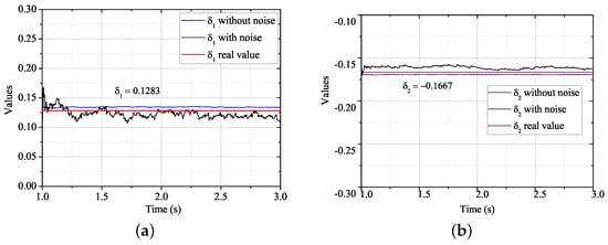
Figure 14.
Error terms estimation in Case 1: (a) Estimation of , (b) Estimation of .
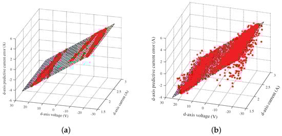
Figure 15.
Original data of d-axis current error equation in Case 1: (a) Data in ideal environment, (b) Data in noise environment.
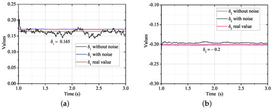
Figure 16.
Error terms estimation in Case 2: (a) Estimation of , (b) Estimation of .
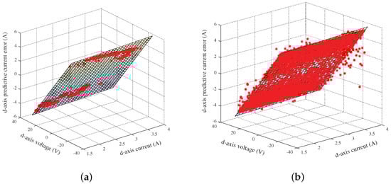
Figure 17.
Original data of d-axis current error equation in Case 2: (a) Data in ideal environment, (b) Data in noise environment.
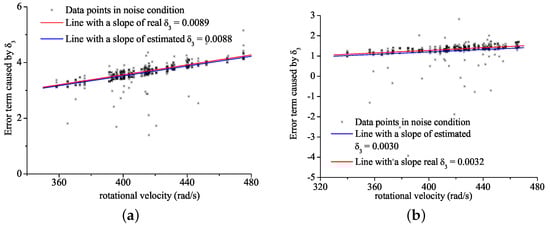
Figure 18.
estimation in noise condition: (a) Estimation results in Case 1, (b) Estimation results in Case 2.
The estimated results are the coefficients of planes in Figure 15a,b, which show the original data in different condition of d-axis current, voltage, and lumped predictive current error caused by and . The left figure indicates that signals were sampled without the disturbance of noise, thus the data are almost located in the estimated plane, while some points deviate from estimated plane in the noisy environment.
Similarly, Figure 16a,b presents the identification process of Case 2. The ideal results also show an opposite steady-state error because of the deviation of d-axis current by the out-of-step rotor position signal. Estimated values in noise condition fluctuate in an allowable range , with and , independently. The real values are , thus the identification error rates are 2.7% and 2.3%, respectively. Figure 17a,b shows the original data of d-axis current error equation in Case 2, which have the same results in Figure 15a,b.
After identifying the first two error factors, the motor is running at near constant velocity, and the q-axis signals are recorded online. The third error factor can be directly derived based on enough data during a short time in a simple linear regressive method. The slopes of the blue lines in Figure 18a,b represent estimated results of the third error factor in noise condition of Cases 1 and 2, respectively. The estimated value of equals 0.0088 in Case 1, which achieves a satisfactory accuracy comparing with the real value of 0.0089. In Case 2, the result also has a high precision with estimation of 0.0030 compare to the real value of 0.0032.
The results of identification are fed to the PMSM’s model online to enhance the accuracy of predictive model. For instance, when the PMSM system was operated in the direct predictive current control (1-PCC) scheme, the nominal parameters took that of Case 1. In Figure 19a,b, before identification is finished, each predictive current in -axis presents a biggish error. However, errors of predictive -axis current are both substantially decreased after the feedback of the previous three estimated values at instant 1.7 s. As shown in Figure 20a, the magnitude of d-axis current error in whole frequency range is highly decreased, which is also shown for the error of q-axis current in Figure 20b. On the other hand, the fall of power spectral density (PSD) of errors of predictive current with noise shown in Figure 21a,b further verifies that identification and compensation are able to enhance the efficiency of electric drive system.
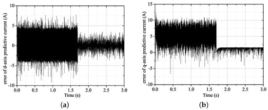
Figure 19.
Errors of predictive current: (a) Error of d-axis predictive current, (b) Error of q-axis predictive current.
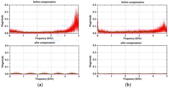
Figure 20.
Analysis in frequency domain of current errors: (a) Changes of d-axis current error after compensation, (b) Changes of d-axis current error after compensation.
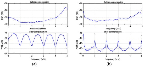
Figure 21.
Analysis of power spectral density (PSD) of current errors with noise: (a) PSD of d-axis current error, (b) PSD of q-axis current error.
6. Conclusions
In this paper, a unified predictive current control scheme based on deadbeat principle for PMSM drive system is proposed. We define an alternative cost function that simplifies the calculation of optimal vectors. The results show that the performance of proposed 1-PCC is not inferior to the conventional PCC. Moreover, its computation time has an advantage over that of C-PCC. The merits of the proposed 2-PCC and 3-PCC are reflected in their much better steady-state accuracy with a little increase computing burden comparing with the 1-PCC. Detailed comparisons of transient and steady capabilities with optimal FOC and DTC-SVM were also conducted, and the results verify that the proposed PCCs have superior output performance. The proposed integrated identification method aiming to approximate the error term in predictive model shows allowable accuracy even in noisy environments. After compensation by the estimated values, the precision of predictive current was significantly improved. The analysis results in frequency domain and PSD further show the increase of system efficiency. In summary, the proposed unified control scheme with compensation is able to ease the application of model predictive control in electric drive system with large-scale parameter uncertainty.
Author Contributions
Conceptualization, P.T. and Y.D.; methodology, P.T.; software, P.T.; validation, P.T. and Z.L.; formal analysis, P.T.; investigation, P.T. and Z.L.; resources, Y.D.; data curation, Y.D.; writing—original draft preparation, P.T.; writing—review and editing, P.T. and Y.D.; visualization, P.T. and Z.L.; supervision, Y.D.; project administration, Y.D.; and funding acquisition, Y.D.
Funding
This research was funded by the Fundamental Research Funds for the Central Universities under Grant A03013023001015.
Conflicts of Interest
The authors declare no conflict of interest.
References
- Bozorgi, A.M.; Farasat, M.; Jafarishiadeh, S. Model predictive current control of surface-mounted permanent magnet synchronous motor with low torque and current ripple. IET Power Electron. 2017, 10, 1120–1128. [Google Scholar] [CrossRef]
- Kouro, S.; Cortes, P.; Vargas, R.; Ammann, U.; Rodriguez, J. Model Predictive Control-A Simple and Powerful Method to Control Power Converters. IEEE Trans. Ind. Electron. 2009, 56, 1826–1838. [Google Scholar] [CrossRef]
- Morel, F.; Lin-Shi, X.; Retif, J.; Allard, B.; Buttay, C. A Comparative Study of Predictive Current Control Schemes for a Permanent-Magnet Synchronous Machine Drive. IEEE Trans. Ind. Electron. 2009, 56, 2715–2728. [Google Scholar] [CrossRef]
- Zhang, Y.; Xu, D.; Liu, J.; Gao, S.; Xu, W. Performance Improvement of Model-Predictive Current Control of Permanent Magnet Synchronous Motor Drives. IEEE Trans. Ind. Appl. 2017, 53, 3683–3695. [Google Scholar] [CrossRef]
- Davari, S.A.; Khaburi, D.A.; Kennel, R. An Improved FCS-MPC Algorithm for an Induction Motor With an Imposed Optimized Weighting Factor. IEEE Trans. Power Electron. 2012, 27, 1540–1551. [Google Scholar] [CrossRef]
- Zhang, Y.; Yang, H. Model predictive torque control of induction motor drives with optimal duty cycle control. IEEE Trans. Power Electron. 2014. [Google Scholar] [CrossRef]
- Liu, Y.; Cheng, S.M.; Zhao, Y.Z.; Liu, J.; Li, Y.S. Optimal two-vector combination-based model predictive current control with compensation for PMSM drives. Int. J. Electron. 2019, 106, 880–894. [Google Scholar] [CrossRef]
- Zhang, Y.; Xu, D.; Huang, L. Generalized Multiple-Vector-Based Mode Predictive Control for PMSM Drives. IEEE Trans. Ind. Electron. 2018, 65, 9356–9366. [Google Scholar] [CrossRef]
- Chen, Z.; Qiu, J.; Jin, M. Adaptive finite-control-set model predictive current control for IPMSM drives with inductance variation. IET Electr. Power Appl. 2017, 11, 874–884. [Google Scholar] [CrossRef]
- Lyu, M.; Wu, G.; Luo, D.; Rong, F.; Huang, S. Robust Nonlinear Predictive Current Control Techniques for PMSM. Energies 2019, 12. [Google Scholar] [CrossRef]
- Zhang, X.; Zhang, L.; Zhang, Y. Model Predictive Current Control for PMSM Drives With Parameter Robustness Improvement. IEEE Trans. Power Electron. 2019, 34, 1645–1657. [Google Scholar] [CrossRef]
- Türker, T.; Buyukkeles, U.; Bakan, A.F. A Robust Predictive Current Controller for PMSM Drives. IEEE Trans. Ind. Electron. 2016, 63, 3906–3914. [Google Scholar] [CrossRef]
- Hoach The, N.; Jung, J.W. Finite Control Set Model Predictive Control to Guarantee Stability and Robustness for Surface-Mounted PM Synchronous Motors. IEEE Trans. Ind. Electron. 2018, 65, 8510–8519. [Google Scholar] [CrossRef]
- Liu, X.; Zhang, Q. Robust Current Predictive Control-Based Equivalent Input Disturbance Approach for PMSM Drive. Electronics 2019, 8. [Google Scholar] [CrossRef]
- Stumper, J.F.; Hagenmeyer, V.; Kuehl, S.; Kennel, R. Deadbeat Control for Electrical Drives: A Robust and Performant Design Based on Differential Flatness. IEEE Trans. Power Electron. 2015, 30, 4585–4596. [Google Scholar] [CrossRef]
- Nalakath, S.; Preindl, M.; Emadi, A. Online multi-parameter estimation of interior permanent magnet motor drives with finite control set model predictive control. IET Electr. Power Appl. 2017, 11, 944–951. [Google Scholar] [CrossRef]
- Gatto, G.; Marongiu, I.; Serpi, A. Discrete-Time Parameter Identification of a Surface-Mounted Permanent Magnet Synchronous Machine. IEEE Trans. Ind. Electron. 2013, 60, 4869–4880. [Google Scholar] [CrossRef]
- Sim, H.W.; Lee, J.S.; Lee, K.B. On-line Parameter Estimation of Interior Permanent Magnet Synchronous Motor using an Extended Kalman Filter. J. Electr. Eng. Technol. 2014, 9, 600–608. [Google Scholar] [CrossRef]
- Liu, Z.H.; Wei, H.L.; Zhong, Q.C.; Liu, K.; Xiao, X.S.; Wu, L.H. Parameter Estimation for VSI-Fed PMSM Based on a Dynamic PSO With Learning Strategies. IEEE Trans. Power Electron. 2017, 32, 3154–3165. [Google Scholar] [CrossRef]
- Liu, K.; Zhu, Z.Q. Position-Offset-Based Parameter Estimation Using the Adaline NN for Condition Monitoring of Permanent-Magnet Synchronous Machines. IEEE Trans. Ind. Electron. 2015, 62, 2372–2383. [Google Scholar] [CrossRef]
- Cortes, P.; Rodriguez, J.; Silva, C.; Flores, A. Delay Compensation in Model Predictive Current Control of a Three-Phase Inverter. IEEE Trans. Ind. Electron. 2012, 59, 1323–1325. [Google Scholar] [CrossRef]
- Ding, F.; Liu, P.X.; Liu, G. Multiinnovation Least-Squares Identification for System Modeling. IEEE Trans. Syst. Man Cybern. Part B (Cybern.) 2010, 40, 767–778. [Google Scholar] [CrossRef] [PubMed]
© 2019 by the authors. Licensee MDPI, Basel, Switzerland. This article is an open access article distributed under the terms and conditions of the Creative Commons Attribution (CC BY) license (http://creativecommons.org/licenses/by/4.0/).