Abstract
This paper presents a proposal for an architecture in FPGA for the implementation of a low complexity near maximum likelihood (Near-ML) detection algorithm for a multiple input-multiple output (MIMO) quadrature spatial modulation (QSM) transmission system. The proposed low complexity detection algorithm is based on a tree search and a spherical detection strategy. Our proposal was verified in the context of a MIMO receiver. The effects of the finite length arithmetic and limited precision were evaluated in terms of their impact on the receiver bit error rate (BER). We defined the minimum fixed point word size required not to impact performance adversely for transmit antennas and receive antennas. The results showed that the proposal performed very near to optimal with the advantage of a meaningful reduction in the complexity of the receiver. The performance analysis of the proposed detector of the MIMO receiver under these conditions showed a strong robustness on the numerical precision, which allowed having a receiver performance very close to that obtained with floating point arithmetic in terms of BER; therefore, we believe this architecture can be an attractive candidate for its implementation in current communications standards.
1. Introduction
A wireless communications system employing multiple antennas achieves a better performance over the wireless channel in terms of capacity and bit error rate (BER) [1] by spreading the transmitted information over space and time in a pattern specified by a space-time block code [2]. Classic examples include V-BLAST, which maximizes the spatial multiplexing gain [3], and the Alamouti code [4], which maximizes the diversity gain. A wide variety of space-time coding techniques has been proposed in the past two decades, each achieving a specific combination of rate and diversity gains and whose decoding requires a certain computational complexity.
Recently, the spatial dimension of MIMO systems was used to modulate the transmitted signal instead of using it for diversity or multiplexing. This technique is known as spatial modulation (SM) [5,6,7]. SM considers the complete array of transmit (Tx) antennas as a spatial constellation, where each Tx antenna in this array represents a point in the spatial constellation. In SM, only one Tx antenna is activated at a time, while the other Tx antennas stay off the air during one symbol transmission. Ideally, there is a different and unique channel between each Tx antenna and a receive (Rx) antenna. Therefore, the receiver can determine which Tx antenna has been utilized in the transmission. In this way, spatially modulated bits add to the received quadrature amplitude modulation (QAM) symbol [8].
Quadrature spatial modulation (QSM) is an SM based transmission technique that uses the quadrature (Q) and the in-phase (I) QAM components to independently modulate a spatial constellation. As a result, QSM has better spectral efficiency (SE) since it transmits twice the number of bits in the spatial domain [9,10,11] with the aim of further improving the performance of SM systems in terms of bit error rate.
The complexity in the receiver is an important factor to take into account for hardware implementations [12], mainly in MIMO and massive MIMO systems where the number of antennas used increases significantly the complexity of the receivers. Some previous works have analyzed this problem for basic QSM transmission schemes. For example, low complexity QSM detectors that consider compressive sensing [13,14], sphere decoding [15], minimum mean squared error (MMSE) [16], equivalent maximum likelihood [17], and zero forcing precoding [18] based low complexity detectors have been recently proposed. However, to the best of our knowledge, practical implementations of hardware architectures for the detection process in MIMO-QSM systems have not been discussed.
Against this background, this research proposes an architecture in FPGA to implement a low complexity near maximum likelihood (Near-ML) detector for a MIMO-QSM system. The proposed low complexity detection algorithm is compared with the ML criterion in terms of BER performance and complexity. Results show that the proposed low complexity Near-ML algorithm performs very near to the optimal detector while achieving a complexity reduction of up to 88% for the analyzed cases.
The contribution of the paper is three-fold:
- A modified low complexity Near-ML detection algorithm based in sphere detectors for the MIMO-QSM system is proposed.
- A new reconfigurable architecture to implement in FPGA the Near-ML detection algorithm is proposed.
- The proposed architecture for the MIMO-QSM receiver can operate for different combinations in transmitter and receiver antennas, including all different sizes of modulation schemes M-QAM, which makes it attractive to be used in the new wireless communication standards.
The remainder of the paper is organized as follows: A description of the QSM general system model with a brief explanation of the QSM implementation, the channel effects at the QSM receiver, and the considerations for an ML detection are presented in Section 2; Section 3 describes the low complexity detection algorithm implemented at the MIMO-QSM receiver; Section 4 show a full description of the proposed architecture for the MIMO-QSM receiver; Section 5 shows the results of BER performance and the proposed architecture to implement the receiver for the MIMO-QSM system. Finally, conclusions are summarized in Section 6.
Notation: Uppercase boldface letters denote matrices, whereas lowercase boldface letters denote vectors. The transpose, Hermitian transpose, and Frobenius norm of are denoted by , , and , respectively. Finally, is used to represent the circularly symmetric complex Gaussian distribution with mean and variance .
2. MIMO-QSM Transmission System
The system model of the MIMO-QSM transmission scheme is presented in Figure 1. We considered a transmitter with transmit antennas and a receiver with receiving antennas. Thus, the end-to- end configuration can be considered as a MIMO transmission system. We assumed a rich scattering, Rayleigh wireless channel with flat and slow fading, where the channel between transmitter antenna j and receiver antenna i can be modeled as a complex Gaussian gain of zero mean and variance 0.5 per dimension. This gain remains constant for several symbol intervals, after which it changes to a new independent channel realization. The system considered here can transmit bits in each time slot, where M is the size of the M-ary quadrature amplitude modulation (QAM) constellation and is the size of the QSM transmission vector. Thus, the general MIMO-QSM communication system can be mathematically modeled as:
which can be expressed equivalently as:
where is the overall transmission vector and is the received vector. is the channel matrix; is the signal-to-noise ratio (SNR) at each antenna; and represents the AWGN vector. The generated noise samples are independent and identically distributed (i.i.d.) with .
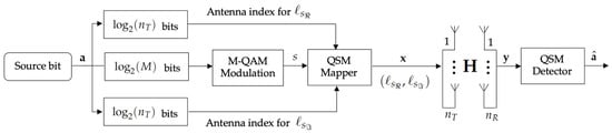
Figure 1.
The MIMO-QSM system model.
Further assumptions were that all the antennas transmit information symbols from the same M-QAM constellation, the receiver has perfect channel state information (CSI), and the receiver is perfectly synchronized to the transmitter.
2.1. QSM Modulation
In order to generate the QSM signals , the input sequence of bits was split into three flows. One flow was utilized to modulate an M-QAM signal, and the other two flows (spatial bits) were used to modulate the position in the output vector . For an input bit sequence of length bits, the first bits modulated an M-QAM symbol. The remaining bits were split into two flows of spatial bits. These spatial bits modulated the position in the output vector as follows: the real part of the QAM symbol was assigned to one specific position in the output vector of length . The imaginary part of the QAM symbol was assigned to another one or even the same position antenna in the output vector . Finally, these two SM signals were combined to obtain the QSM output vector [9].
Table 1 shows a mapping rule example for QSM using four-QAM and . The first column shows the input bit sequence of length , where the first two bits modulate a four-QAM symbol and the remaining two bits modulate the position of the non-zero entries in the output vector as follows: the real part of the QAM symbol was assigned to one Tx antenna out of available in order to modulate bit, whereas the imaginary part of the QAM symbol was assigned to another or even the same position to modulate bit to define the and index transmitter antenna, respectively, as shown in the third column of Table 1.

Table 1.
Example of the QSM mapping rule with .
2.2. ML Detection
The MIMO transmitted signal is:
where the transmitted symbol can be split into two real valued signals, and , according to the QSM mapping rule described in Table 1. Since the QAM symbol s is expanded by the matrix , (3) can be expressed as:
where and denote the and columns of , respectively, with , and the vectors and of dimension and , respectively, represent the different real and imaginary parts of the symbols belonging to the M-QAM constellation ; finally, the symbol · represents the product among the and columns of and each element of the vectors and .
Assuming that the receiver had perfect channel state information, the ML estimation compared the distance between the received signal and all possible received signals. The ML criterion is defined as:
where is the Euclidean distance among two vectors and is the full spatial modulation QSM used in the transmitter; therefore, the ML detector jointly estimated the two possible active Tx antenna indices, and , and the corresponding real valued signals and . Therefore, (5) can be written as:
3. Low Complexity Detection Algorithm
In recent works, some low complexity algorithms have been presented for MIMO, SM, and QSM signal detection [10,13,19]. In the works presented by [14,16], optimization algorithms and trigonometric functions were required in the receiver to detect the most likely antenna combinations. After the antenna indices were detected, a reduced ML detector was utilized to identify the transmitted symbols in the MIMO-QSM system. However, these schemes demand many hardware implementation resources. Other detection techniques for MIMO-SM-QSM were reported in [15,19,20]. These detectors were based on tree search and spherical detection. These algorithms had an excellent BER performance, and their detection complexity in terms of flops were relatively simple for hardware implementation in FPGA.
In this section, a modified low complexity Near-ML detector for MIMO-QSM signals is presented. The proposed detector is based on a tree search and a spherical algorithm [20,21].
The ML solution to (6) may be expressed as a tree search: each branch in this tree was assigned a distance metric where the symbols with the smallest overall distance were selected as possible optimum solutions [22] in each level of the tree. To carry out this process, an adaptive M-algorithm based on a breadth first sorted tree search was used. The proposed algorithm reduced the search complexity by storing only, at maximum, the best L branches at a time [23] in each level of the tree. Henceforth, a small L resulted in low complexity and relatively sub-optimal performance. As L increased, the complexity of the detector in terms of flops also increased, and the performance of the algorithm approached the ML solution.
The decision metrics and , required in the Near-ML proposal detector for the MIMO-QSM scheme can be established as follows:
We denote the and element in the vectors and by and , respectively. The goal of the decoder is to find the optimum solution to the ML criterion in (6), using the distances calculated in (7) and (8). For the case of the distance , it is a vector of distances calculated for each valid combination between the transmitter antenna and each element of the vector . The decoding procedure was split into two parts. First, a pre-ordering with was carried out; specifically, the distance of (7) was calculated, and symbols were re-ordered in ascending order. In this way, a set of tuples was obtained, each tuple being formed of a combination of the Tx antenna index and the Tx symbol . This part is summarized in Algorithm 1.
The second part corresponds to an optimized detector based on the detector for SM signals published in [21]. Since the first part of the Near-ML algorithm estimated the real part of the transmitted QSM symbol, , the second part considered that only one Tx antenna was active, which corresponded to the imaginary part of the QSM transmitted symbol . Therefore, the proposed method performed the search using the following modified Rx vector:
The decision metrics required in the second part or the Near-ML proposal detector for the MIMO-QSM scheme can be established as follows:
| Algorithm 1 QSM real part decoding. |
| Require: Channel matrix , received vector , , Ensure: The set of tuples ordered 1: Let , 2: for do 3: Let 4: for do 5: Let 6: end for 7: end for 8: Let in ascending order. 9: Order with the same order of 10: Return , |
For the case of the distance , it was a vector of distances calculated for each valid combinations between the transmitter antenna and each element of the vector . This part of the Near-ML algorithm is summarized in Algorithm 2. We denote the column of like and the row of and like as and , respectively.
| Algorithm 2 QSM imaginary part decoding. |
| Require: Channel matrix , modified received vector , , , Ensure: The optimum tuple , 1: Let , 2: for do 3: Let 4: for do 5: Let 6: end for 7: end for 8: Let in ascending order. 9: Order with the same order of 10: Let 11: for do 12: Let 13: for do 14: Let and 15: Let 16: Let 17: if then 18: Let 19: Let and 20: else if then 21: 22: 23: end if 24: end for 25: end for 26: Return , |
The complete Near-ML detector is described with detail in Algorithm 3. Each iteration produced a symbol estimation with distance . Symbol pairs whose distance were not smaller than the previous ones were skipped. In each iteration, we used the criterion ( and ). The detector used the metrics of the sphere detector to stop the search and discard branches of the tree that were not viable solutions because they exceeded the maximum radius of the detection sphere according to [15,24]. With this modification, the number of branches for each level was adaptive and depended on the SNR and the channel. For these reasons, the proposed algorithm had a significantly reduced complexity.
| Algorithm 3 Complete Near-ML detector. |
| Require: Channel matrix , modified received vector , , , , q, , , Ensure: Optimum 1: Let 2: Let and 3: Execute the QSM real part decoding to obtain , 4: Let 5: for do 6: Let 7: Let 8: Execute the QSM imaginary part decoding to obtain , 9: if then 10: Let 11: Let 12: Let 13: Let 14: Let 15: if then 16: break 17: end if 18: else if and then 19: break 20: end if 21: end for 22: Return |
It is also worth noting that in the proposed algorithm, it is possible to adjust the complexity/BER performance trade-off of the detector the maximum limit of the thresholds and . The advantages of our proposal with respect to other similar schemes recently proposed were: It did not require calculating the QR decomposition; therefore, it was less complex. Additionally, it did not require using complex operations; therefore, it was most adequate for hardware implementation.
In the next subsection, BER performance results and the detection complexity of the proposed scheme were compared to the conventional MIMO-QSM scheme for the ML detection algorithm. Furthermore, the BER performance and the complexity of the proposed low-complexity detection algorithm were analyzed.
3.1. BER Performance Comparison of the MIMO-QSM Scheme
In this subsection, two different configurations were used in order to compare the BER performance of the proposed MIMO-QSM scheme for the ML detection under uncorrelated Rayleigh fading channels. The systems were analyzed considering the same spectral efficiency, the same number of Tx and Rx antennas, and a normalized transmission power in the transmitter. For all computer simulations, we targeted a BER of .
Figure 2 shows the performance comparison for the optimal ML and the proposed low complexity Near-ML algorithm for the MIMO-QSM scheme using the and configuration with QPSK modulator. For both cases, the proposed detector performed very near to the ML algorithm, and for this reason, we called our proposal detector Near-ML.
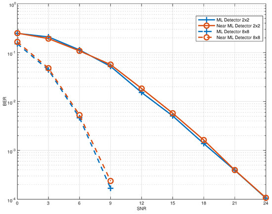
Figure 2.
Performance comparison for an and configuration at and bpcu respectively.
3.2. Complexity
The ML detection complexity for the ML criterion in (6) was measured in terms of complex operations (CO). One arithmetic operation was considered as one CO; also, one comparison was considered as one CO. The lattice in the system had points. Subtraction, obtaining the square, and finding the minimum in (6) resulted in CO. Considering receive antennas, the complexity for ML in (6) can be approximated by:
Table 2 shows a comparison of the complexity for two MIMO configurations. In Table 2, the QSM scheme with ML detector is considered as the reference with 100% of complexity for an SNR of 9 dB. The last column shows the complexity of the proposed Near-ML algorithm where it is observed how this detector outperformed significantly the QSM ML detector in terms of complexity.
Table 2.
Comparison of complexity .
The results showed that the proposed Near-ML algorithm performed very near to the optimal one with the advantage of a reduction in detection complexity of 88%.
4. Proposed Hardware Architecture for the Digital QSM Detector
A hardware architecture that implements the detection algorithm presented in Section 3 was proposed. In order to illustrate it, the top module is shown first, and then, the internals of each module are explored.
The design of the architecture followed a top-down approach, and it was composed of the data-path that included four modules and a control unit. The detector is presented in Figure 3. The det1and det2 modules implemented the first and second parts of the detection process, described in Algorithms 1 and 2, respectively; the sort module performed the sort operation used in the three algorithms; the fd module compared the distance metrics needed to determine the received symbol (inside the for cycle in Algorithm 3); and the ctrl module provided the timing signals and activation flags for the data-path.
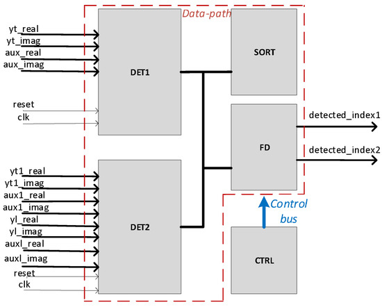
Figure 3.
QSM detector architecture.
From this point onwards, a bold line represents a bit vector, whereas a thin line represents a single bit.
4.1. Top View of the QSM Detector Architecture
Using the description of the QSM communication system in Section 2.1 and the architecture proposed in Figure 3, a top view of the detector is presented considering the following parameters:
- NT: number of Tx antennas.
- NR: number of Rx antennas.
- WL: word length used for fixed point representation.
- IP: amount of bits used to represent the integer part of data.
- FP: amount of bits used to represent the fractional part of data. Result of subtracting WL and IP.
- HXQC: number of columns of an auxiliary matrix needed for calculations in det1.
- HXQ1S: size of an auxiliary vector needed for calculations in det2.
Considering Table 3, which summarizes the inputs and outputs of the whole system, the detection process started when the received signal y was mapped into ports yt_real and yt_imag. This input signal was then processed by det1, which executed Algorithm 1 in hardware. After that, det2 received data in its yt1_real and yt1_imag (equivalent to the modified received vector y) ports to continue with Algorithm 2.
Table 3.
Inputs and outputs of the detector.
The sort operation was utilized by both detection processes; therefore, sort can be used by det1 and det2.
At the final step of the detection process, the fd module compared the current detection results with predefined parameters (, , , in Algorithm 3); if the process matched these parameters, the current results became the final results; otherwise, the detection process was restarted until the conditions were met. The ctrl module controlled and synchronized the whole interoperability of the architecture.
The outputs detected_index1 and detected_index2 represent the pair [transmit antenna, symbol sent] for QSM.
In what follows, the modules of the detector are described in detail.
4.2. det1 Module
The detection started with det1, implementing Algorithm 1. Its architecture is shown in Figure 4, and an explanation of the inputs and outputs is in Table 4.
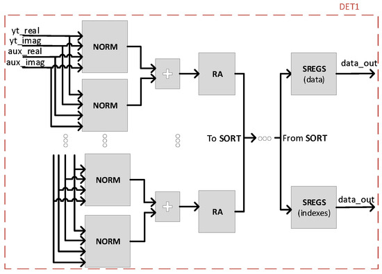
Figure 4.
Architecture of det1.
Table 4.
Inputs and outputs of det1.
Modules:
- Norm (norm): operation of Euclidean distance.
- RegisterArray (ra): register array for the results of norm.
- SortingRegs (sregs): register array for the results of sort.
When the detection started, the norm modules computed the Euclidean distance operation between (yt_real, yt_imag) and (aux_real, aux_imag) corresponding to the norm operation presented in Line 3 of Algorithm 1.
The results were then added and stored in the corresponding ra registers in an orderly manner. When every register had data stored, these results were sent to the sort module in a parallel way, as better described in Section 4.4.
When the sorted data returned, as seen in “From sort” in Figure 4, the data and indexes were stored, in the same order as they came out of the sorting module, in their respective sregs, which was another register array.
4.3. det2 Module
The second detection process, det2, was at the same time divided into two parts representing the for cycles in Lines 2 and 11, respectively, of Algorithm 2. Figure 5 shows the first part (det2_p1) with the first norm blocks and the second part (det2_p2) with the last block. When det2_p1 ended, det2_p2 immediately started. Table 5 shows the inputs and outputs of the module.
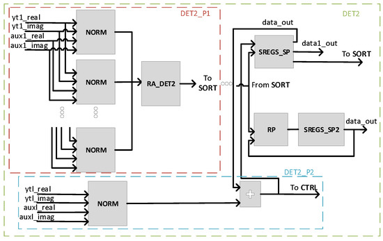
Figure 5.
Architecture of det2.
Table 5.
Inputs and outputs of det2.
Modules:
- Norm (norm): operation of Euclidean distance.
- RegisterArray for det2 (ra_det2): register array for the results of norm in det2_p1.
- SortingRegs_SP (sregs_sp): register array for the sorting results in det2.
- SortingRegs_SP2 sregs_sp2: register array for the sorting indexes results in det2.
- RearrangerP(rp): rearranger for the sorting indexes.
After the calculations with the norm modules were done, ra_det2 sent its stored data to sort. When the data came back from the module, they were split into the data vector and index vector to be stored in sregs_sp and sregs_sp2, respectively.
sregs_sp was a register array that had both serial and parallel inputs and outputs and stored the sorting data. It also had outputs like data1_out that fed the control module, equivalent to in Algorithm 2, Line 19.
sregs_sp2 stored the indexes given by the sort module. It only had a parallel input, but serial and parallel outputs; this configuration helps when you need to reorder all indexes (parallel output, as in Line 9 of Algorithm 2) or you need to read only one index.
In det2_p2, another norm module was used, and its result was added to one of the already stored in sregs_sp, then fed back to the same register and sent to sorting again, emulating the behavior of Lines 14 and 15 of Algorithm 2.
When coming back from sorting, rp rearranged the old indexes stored in sregs_sp2 based on the new ones and replaced them. For example, if the stored vector was and the new indexes were , then the rearranged vector would be .
4.4. sort Module
The sort module was the most used during the detection process. Sorting networks were chosen as the option for sorting in FPGA [25].
A sorting network is one of the most efficient and traditional ways of sorting in FPGA. They are attractive due two main reasons: they do not require control instructions, and they are relatively easy to parallelize due to the simplicity of the data flow. Sorting networks are adequate for sorting short arrays, the length of which is known beforehand.
According to the detection algorithm, besides sorting, the network must indicate in which position of the array the elements were originally, before entering the network and being sorted; similar to how MATLAB does it with its integrated function [26]. There was already a work that addressed this problem in hardware [27], so the architecture proposed there was used here.
The implemented sorting network consisted of purely combinational comparators so, as the network grew according to the sorting needs, the critical route of the system increased as well.
Figure 6 shows the structure of the sorting network, and Table 6 describes the inputs and outputs of the module.
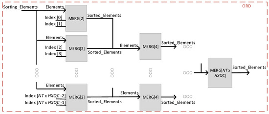
Figure 6.
Architecture of sort.
Table 6.
Inputs and outputs of sort.
The vector Sorting_Elements came from the registers in det1 and det2, and Sorted_Elements was composed of the sorted data and their respective indexes that were going to be stored in sregs.
4.5. fd and ctrl Modules
The fd module made the decision of accepting the current detected indexes as valid or not. It achieved this by comparing the detection results with predefined parameters specific to QSM detectors (, , , in Algorithm 3). In case the results were accepted, the detection process ended; otherwise, det2 started over with different data. This was implemented with counters and a state machine, so it emulated the behavior of the for cycle in Algorithm 3.
The ctrl module grouped three independent modules that controlled the three main parts of the detector (det1, det2_p1, and det2_p2).
The control modules for det1 and det2_p1 were composed mainly of counters that checked the number of elapsed clock cycles, representing their respective for cycles in the algorithms.
The control module for det2_p2 differed from the other two control modules. This one consisted of a state machine and counters that performed the for cycles in Algorithm 2, specifically Lines 11 and 13. As is seen in Line 13, the lim variable was known until execution time and changed depending on the data, the reason why a state machine was required for proper control.
5. Analysis of Hardware Implementation and Verification Results
5.1. Hardware Budget
In order to implement the proposed design, an Intel-Altera Cyclone IV EP4CE115 FPGA was used. In Table 7, the amount of resources, maximum frequency, and throughput, are shown for two representative cases of the QSM communication systems. The number in brackets represents the percentage of resources used out of the total available in the FPGA device.
Table 7.
Overall implementation results of the detector in a Cyclone IV FPGA.
Table 8 presents a breakdown of post-synthesis resources used by the different modules of the architecture for the 2 × 2 QPSK and 2 ×2 16-QAM configurations, respectively. Naturally, the amount of resources went up as the order of modulation and the number of antennas increased.
Table 8.
Resources used per module of the architecture.
According to the results, the SORT block was the module with the greatest amount of hardware resources. It used only combinational components (as it was based on sorting networks) [27] to make a comparison between elements and increased in size as the number of elements to sort rose. Given these characteristics, the critical route of the whole implementation was established by this module and affected the general performance of the architecture.
Due to the algorithm being inherently recursive, the number of clock cycles was data dependent. Table 7 shows the max frequency considering the slow 1200 mV 0C model; and throughput, which is the number of detection processes that can be done per second in the worst case.
5.2. Simulation Results
In order to verify the results, a MATLAB implementation was used to generate random input vectors written in text files for the architecture. These files were fed into a test bench that controlled the reading of the test vectors and the writing of the results.
Figure 7 summarizes the testing process to obtain the results and compare them with the outputs of the MATLAB algorithm.
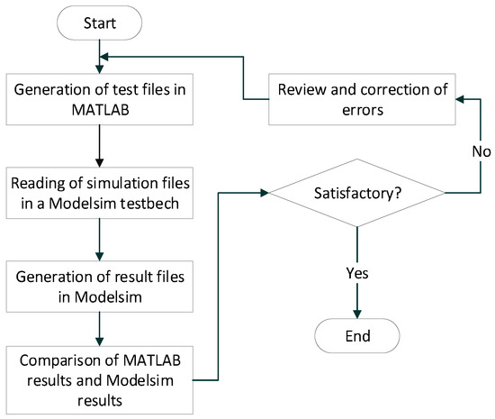
Figure 7.
Process of the generation of simulation results.
Fixed point simulations were performed in order to determine the ideal IP and FP parameters depending on the BER performance of the algorithm. Figure 8 shows the comparison for different configurations of word length against the floating point model used (4 × 4, QPSK). Taking as a reference Figure 8, the fixed point format IP = 5 and FP = 11 had a close performance to the floating point model.
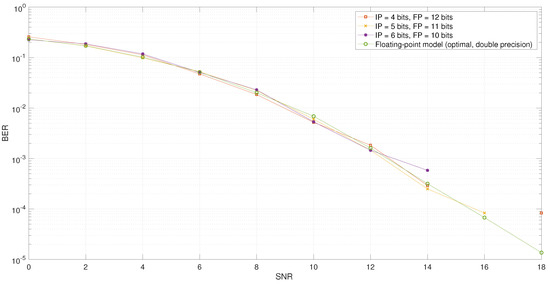
Figure 8.
Fixed point analysis for the algorithm, 16-bit word length, 4 × 4, QPSK.
Figure 9 shows the timing diagram of the detection process. When start = 1, yt_real and yt_imag were processed by det1 and after five cycles in the case of a QPSK modulation, the flag done_detection1 was set to one (END_DET1 in Figure 9), indicating that det2_p1 could start. At this point, Algorithm 1 was performed.
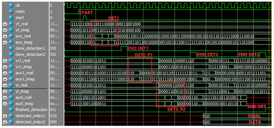
Figure 9.
Simulation in Modelsim of the proposed detector.
The det2_p1 module read the yt1_real and yt1_imag inputs and processed them according to Algorithm 2. Immediately after, det2_p2 did the same with the yl_real and yl_imag inputs and set done_detection2 to one (END DET2) when it finished, informing the fd module that the data were ready for it to make a decision. At this point, Algorithm 2 was performed.
The fd module required one clock cycle to make the decision of accepting the current detected indexes or not. In the case of this simulation, said indexes were not accepted at first, so it sent the appropriate signals to start det2 over.
det2 read its respective signals and was performed again. When it finished (represented by the rightmost END DET2 in Figure 9), the fd module took another clock cycle to decide. This time, the detected indexes were accepted, as the finished_detection flag was raised, meaning that the detection process (Algorithm 3) was over and the detected data (FINAL DATA in Figure 9) were valid.
6. Conclusions
A low complexity detection algorithm based on a tree search and spherical detection, in the context of MIMO QSM transmission, was presented. It was shown that the proposed algorithm achieved a similar performance to the ML detector, but with a significant complexity reduction in terms of the operations required in its software and hardware implementation. Fixed point analysis showed that BER performance was maintained on the detection process, allowing a simpler hardware implementation rather than the hardware needed for an implementation using floating point precision. The novel hardware architecture showed the feasibility of the hardware implementation of the proposed algorithm using fixed point precision and the process of transformation from the algorithm to hardware architecture.
A possible workaround for the critical route would be the implementation of pipeline stages inside the sorting module in order to improve the maximum frequency and throughput significantly, even if the added registers would mean a redesign of the control unit.
Author Contributions
Conceptualization, I.L., J.C. and L.P.-E.; Methodology, I.L., J.C. and L.P.-E.; Software, I.L. and J.C.; Experimentation, I.L., J.C., L.P.-E. and O.L.-G.; Validation, I.L., J.C., L.P.-E. and O.L.-G.; Formal Analysis, I.L., J.C., L.P.-E., O.L.-G. and A.G.; Investigation, I.L., J.C., L.P.-E., O.L.-G. and A.G.; Resources, J.C. and A.G.; Data Curation, I.L.; Writing—Original Draft Preparation, I.L.; Writing—Review & Editing, I.L., J.C., L.P.-E. and O.L.-G.; Visualization, I.L., J.C., L.P.-E., O.L.-G. and A.G.; Supervision, I.L., J.C., L.P.-E. and O.L.-G.; Project Administration, J.C. and A.G.; Funding Acquisition, J.C. and A.G.
Funding
The present article was jointly funded by PFCE 2019, CONACYT scholarship and PROFAPI 2019.
Conflicts of Interest
On behalf of all authors, the corresponding author states that there is no conflict of interest.
References
- Wang, C.X.; Haider, F.; Gao, X.; You, X.H.; Yang, Y.; Yuan, D.; Aggoune, H.M.; Haas, H.; Fletcher, S.; Hepsaydir, E. Cellular architecture and key technologies for 5G wireless communication networks. IEEE Commun. Mag. 2014, 52, 122–130. [Google Scholar] [CrossRef]
- Zheng, L.; Tse, D.N.C. Diversity and multiplexing: A fundamental tradeoff in multiple-antenna channels. IEEE Trans. Inf. Theory 2003, 49, 1073–1096. [Google Scholar] [CrossRef]
- Foschini, G.J. Layered space-time architecture for wireless communication in a fading environment when using multi-element antennas. Bell Labs Tech. J. 1996, 1, 41–59. [Google Scholar] [CrossRef]
- Alamouti, S.M. A simple transmit diversity technique for wireless communications. IEEE J. Sel. Areas Commun. 1998, 16, 1451–1458. [Google Scholar] [CrossRef]
- Basar, E.; Wen, M.; Mesleh, R.; Di Renzo, M.; Xiao, Y.; Haas, H. Index Modulation Techniques for Next-Generation Wireless Networks. IEEE Access 2017, 5, 16693–16746. [Google Scholar] [CrossRef]
- Bai, Z.; Peng, S.; Zhang, Q.; Zhang, N. OCC-Selection-Based High-Efficient UWB Spatial Modulation System Over a Multipath Fading Channel. IEEE Syst. J. 2019, 13, 1181–1189. [Google Scholar] [CrossRef]
- Wen, M.; Zheng, B.; Kim, K.J.; Di Renzo, M.; Tsiftsis, T.A.; Chen, K.; Al-Dhahir, N. A Survey on Spatial Modulation in Emerging Wireless Systems: Research Progresses and Applications. IEEE J. Sel. Areas Commun. 2019, 37, 1949–1972. [Google Scholar] [CrossRef]
- Renzo, M.D.; Haas, H.; Ghrayeb, A.; Sugiura, S.; Hanzo, L. Spatial Modulation for Generalized MIMO: Challenges, Opportunities, and Implementation. Proc. IEEE 2014, 102, 56–103. [Google Scholar] [CrossRef]
- Mesleh, R.; Ikki, S.S.; Aggoune, H.M. Quadrature Spatial Modulation. IEEE Trans. Veh. Technol. 2015, 64, 2738–2742. [Google Scholar] [CrossRef]
- Castillo-Soria, F.; Cortez, J.; Gutierrez, C.; Luna-Rivera, M.; Garcia-Barrientos, A. Extended quadrature spatial modulation for MIMO wireless communications. Phys. Commun. 2019, 32, 88–95. [Google Scholar] [CrossRef]
- Hussein, H.S.; Elsayed, M.; Mohamed, U.S.; Esmaiel, H.; Mohamed, E.M. Spectral Efficient Spatial Modulation Techniques. IEEE Access 2019, 7, 1454–1469. [Google Scholar] [CrossRef]
- Mesleh, R.; Hiari, O.; Younis, A. Generalized space modulation techniques: Hardware design and considerations. Phys. Commun. 2018, 26, 87–95. [Google Scholar] [CrossRef]
- Xiao, L.; Yang, P.; Fan, S.; Li, S.; Song, L.; Xiao, Y. Low-Complexity Signal Detection for Large-Scale Quadrature Spatial Modulation Systems. IEEE Commun. Lett. 2016, 20, 2173–2176. [Google Scholar] [CrossRef]
- Yigit, Z.; Basar, E. Low-complexity detection of quadrature spatial modulation. Electron. Lett. 2016, 52, 1729–1731. [Google Scholar] [CrossRef]
- Al-Nahhal, I.; Dobre, O.A.; Ikki, S.S. Quadrature Spatial Modulation Decoding Complexity: Study and Reduction. IEEE Wirel. Commun. Lett. 2017, 6, 378–381. [Google Scholar] [CrossRef]
- Li, J.; Jiang, X.; Yan, Y.; Yu, W.; Song, S.; Lee, M.H. Low Complexity Detection for Quadrature Spatial Modulation Systems. Wirel. Pers. Commun. 2017, 95, 4171–4183. [Google Scholar] [CrossRef]
- Zheng, B.; Chen, F.; Wen, M.; Ji, F.; Yu, H.; Liu, Y. Low-Complexity ML Detector and Performance Analysis for OFDM With In-Phase/Quadrature Index Modulation. IEEE Commun. Lett. 2015, 19, 1893–1896. [Google Scholar] [CrossRef]
- Li, J.; Wen, M.; Cheng, X.; Yan, Y.; Song, S.; Lee, M.H. Generalized Precoding-Aided Quadrature Spatial Modulation. IEEE Trans. Veh. Technol. 2017, 66, 1881–1886. [Google Scholar] [CrossRef]
- Al-Nahhal, I.; Basar, E.; Dobre, O.A.; Ikki, S. Optimum Low-Complexity Decoder for Spatial Modulation. IEEE J. Sel. Areas Commun. 2019, 37, 2001–2013. [Google Scholar] [CrossRef]
- Jiang, Y.; Lan, Y.; He, S.; Li, J.; Jiang, Z. Improved Low-Complexity Sphere Decoding for Generalized Spatial Modulation. IEEE Commun. Lett. 2018, 22, 1164–1167. [Google Scholar] [CrossRef]
- Zheng, J.; Yang, X.; Li, Z. Low-complexity detection method for spatial modulation based on M-algorithm. Electron. Lett. 2014, 50, 1552–1554. [Google Scholar] [CrossRef]
- Anderson, J.; Mohan, S. Sequential Coding Algorithms: A Survey and Cost Analysis. IEEE Trans. Commun. 1984, 32, 169–176. [Google Scholar] [CrossRef]
- Hassibi, B.; Vikalo, H. On the sphere-decoding algorithm I. Expected complexity. IEEE Trans. Signal Process. 2005, 53, 2806–2818. [Google Scholar] [CrossRef]
- Xiao, L.; Yang, P.; Xiao, Y.; Fan, S.; Di Renzo, M.; Xiang, W.; Li, S. Efficient Compressive Sensing Detectors for Generalized Spatial Modulation Systems. IEEE Trans. Veh. Technol. 2017, 66, 1284–1298. [Google Scholar] [CrossRef]
- Mueller, R.; Teubner, J.; Alonso, G. Sorting Networks on FPGAs. VLDB J. 2012, 21, 1–23. [Google Scholar] [CrossRef]
- MathWorks. Sort Array Elements—MATLAB Sort. Available online: https://www.mathworks.com/help/matlab/ref/sort.html (accessed on 6 September 2018).
- López Mendoza, I.; Pizano Escalante, J.L.; Cortez González, J.; Longoria Gándara, O.H. Implementation of a parameterizable sorting network for spatial modulation detection on FPGA. In Proceedings of the 2019 IEEE Colombian Conference on Communications and Computing (COLCOM), Barranquilla, Colombia, 5–7 June 2019; pp. 1–6. [Google Scholar]
© 2019 by the authors. Licensee MDPI, Basel, Switzerland. This article is an open access article distributed under the terms and conditions of the Creative Commons Attribution (CC BY) license (http://creativecommons.org/licenses/by/4.0/).