Memory Optimization for Bit-Vector-Based Packet Classification on FPGA

Abstract

High-performance packet classification algorithms have been widely studied during the past decade. Bit-Vector-based algorithms proposed for FPGA can achieve very high throughput by decomposing rules delicately. However, the relatively large memory resources consumption severely hinders applications of the algorithms extensively. It is noteworthy that, in the Bit-Vector-based algorithms, stringent memory resources in FPGA are wasted to store relatively plenty of useless wildcards in the rules. We thus present a memory-optimized packet classification scheme named WeeBV to eliminate the memory occupied by the wildcards. WeeBV consists of a heterogeneous two-dimensional lookup pipeline and an optimized heuristic algorithm for searching all the wildcard positions that can be removed. It can achieve a significant reduction in memory resources without compromising the high throughput of the original Bit-Vector-based algorithms. We implement WeeBV and evaluate its performance by simulation and FPGA prototype. Experimental results show that our approach can save 37% and 41% memory consumption on average for synthetic 5-tuple rules and OpenFlow rules respectively.

1. Introduction

Packet classification is one of the core functions required by popular network services such as Quality of Service (QoS), Access Control List (ACL) and traffic monitoring. Besides, packet classification is a core problem for OpenFlow-based [1] software-defined networking [2], which required many packet header fields to be examined against thousands of rules in a ruleset. The growing number of fields [3] and the expanding rulesets pose a great challenge to a practical packet classification solution with high throughput and low memory consumption.

Many effective studies have been proposed for the classical problem in the past decade. Software packet classification algorithms, such as decision-tree-based algorithms and tuple space search algorithms [3,4,5,6] have been proposed for CPU processing platforms. However, the performance of the software-based approaches is limited by the memory system of CPU. Ternary Content Addressable Memory (TCAM)-based solutions have been widely adopted in the industrial field [7,8] for implementing ACLs, as the TCAMs enable parallel lookups on rules for wire-speed classification. However, they are expensive, power-hungry and capacity-limited. Field Programmable Gate Array (FPGA) has been widely used to overcome performance problems of real-time network processing applications [9,10,11]. Bit-Vector-based (BV-based) algorithms [12,13,14] have been proposed for packet classification on FPGA by exploiting hardware parallelism based on rules decomposition. Although the abovementioned algorithms require to store at least $2\ast L$ N-bit-vector in FPGA (L is the total number of the bits of all match fields, and N is the number of the ruleset [13]), they can achieve high throughput by utilizing a homogeneous pipeline structure consisting of classification Processing Engines (PEs). Nevertheless, with increasing matching fields and rulesets, the main clock frequency of the FPGA degrades due to the expenditure incurred by placing and routing with FPGA.

To address the above issue, the state-of-the-art research [15] partitions N-bit-vector into smaller sub-vectors to improve the overall performance of the classification PEs in FPGA. However, the approach does not reduce the memory resources required. Instead, more overhead of memory and logic resources are required due to the partition and the dynamic update function introduced.

In this paper, we present a memory-optimized scheme called Wildcard-removed Bit-Vector (WeeBV) to accommodate larger rulesets for packet classification on FPGA. WeeBV removes the memory storing the wildcards as much as possible by fully exploiting the characteristics of the rulesets. Moreover, it can provide an efficient dynamic update by utilizing the intrinsic dynamic reconfiguration capability of FPGA. Our contributions in this work include:

• Heterogeneous Two-dimensional Pipeline for matching rules, WeeTP. WeeTP converts some standard PEs (proposed in [15]) with the memory storing BV and lookup logic to wildcard PEs. A wildcard PE integrates only registers and fixed logic wires while the SRAM memory is eliminated.
• Optimized heuristic Maximum Covering algorithm for searching wildcards to be removed, WeeMC. WeeMC tries to find the wildcard groups as much as possible by adjusting the order of the rules, where each group occupies a whole SRAM block to be removed. The search space is extremely large and the search problem is NP-hard. WeeMC utilizes a greedy idea for a near-optimal solution.
• Dynamic Sink-Update strategy, WeeSU. WeeSU is proposed to support dynamic updates function for WeeBV. Furthermore, it utilizes the dynamically reconfigurable feature of the state-of-the-art FPGA for accommodating drastic updates.

We evaluate our scheme using synthetic 10 K 5-tuple rules from ClassBench [16] and 10 K OpenFlow1.0 rules from ClassBench-ng [17]. Considering that the recent studies [18,19] have been validated against dozens of thousands of rules, it is reasonable to choose rules around 10K. Compared with StridBV [14], WeeBV can save on average 37% and 41% of storage resources on the two typical rulesets respectively.

The rest of the paper is organized as follows. Section 2 reviews the BV-based approaches and discusses the motivation of this paper. In Section 3, we detail the WeeBV including the WeeTP, WeeMC, and WeeSU. Optimization techniques are proposed in Section 4. We present experimental results in Section 5. Section 6 surveys the related works. Finally, the paper is concluded in Section 7.

2. Background and Motivations

2.1. BV-Based Approaches and Challenges

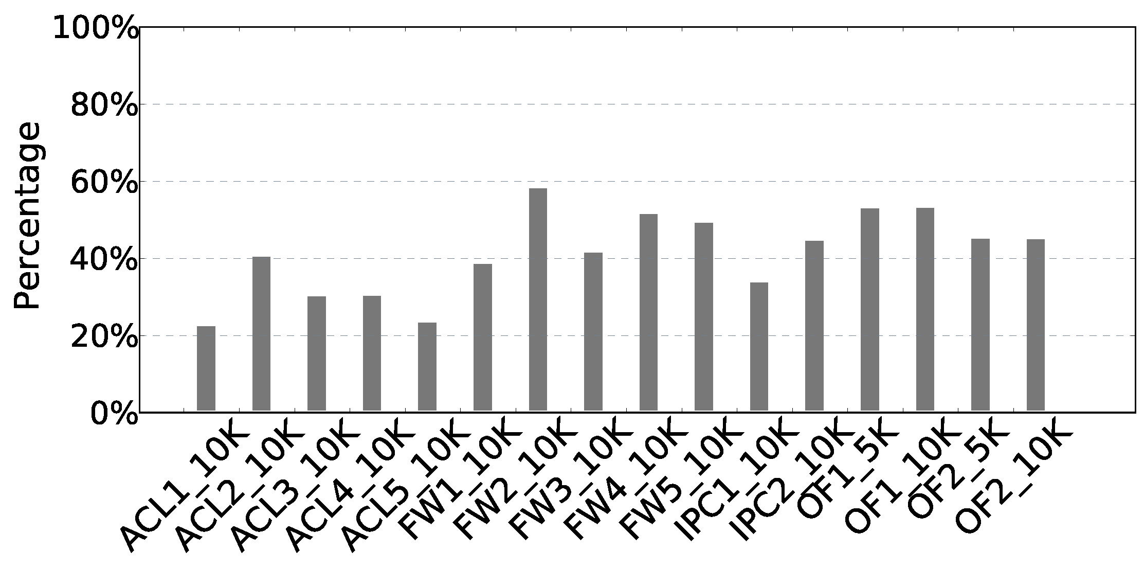
In the BV-based approaches, matching fields (e.g., source IP address) are split into $\frac{L}{s}$ sub-fields, where s$(1\ll s\ll L)$ denotes the length of a sub-field. We use $K_j$ (j = 0, 1, …, $\frac{L}{s}-1$) to denote the s bits of sub-field j. The FSBV algorithm [13] is a special case where s is 1, which creates bit-level subdimension partitioning. The s is increased in the StrideBV algorithm [14] for better performance. Furthermore, the state-of-the-art research [15] splits a ruleset into $\frac{N}{n}$ sub-rulesets for improving the scalability on large rulesets.

An example of BV-based packet classification approach is illustrated in Figure 1a. A bit-vector ${B{V}_i}^{K_j}$ is used to represent the matching result of $K_j$ for the corresponding matching sub-field${}_j$ of the sub-ruleset${}_i$. The values of ${B{V}_i}^{K_j}$ can be calculated by algorithms in [14]. $B{V}_{(i,j)}$ is used to denote a bit-vector table accommodating all values of ${B{V}_i}^{K_j}$. In this example, s is set to 2 and n is set to 3. For example, in Figure 1a, if the input packet header has $K_0$ = 01 in the sub-field 0 of the sub-ruleset 1, we extract the ${B{V}_1}^{K_0}$ = 001; this indicates only the rule $R_5$ of the sub-ruleset 1 matches the input in this sub-field. The memory consumption of the BV tables can be calculated using the following equation:

$$M_{BV}=\frac{N}{n}\ast \frac{L}{s}\ast n\ast 2^s=L\ast N\ast \frac{2^s}{s}$$

(1)

According to Equation (1), memory usage increases as the number of rules increases. In this case, BV-based algorithms can get the smallest memory consumption (i.e., $2\ast L\ast N$) when $s=1$. Worse, when s is increased to improve performance, the memory consumed by BV-based algorithms grows exponentially with s, which poses a huge challenge for large rulesets.

2.2. Motivation

As can be seen from Figure 1a, the matching result of packet classification is determined by bit 0s and bit 1s (rather than wildcards) in a rule. Wildcards do not influence the matching process. Furthermore, wildcards occupy a considerable percentage in typical rulesets. We show the statistical results of the various rulesets generated by the CLassBench [16] and ClassBench-ng [17] in Figure 2, including Accesses Control List (ACL), Firewall (FW), IP Chain (IPC) and OpenFlow1.0 9 (OF). The traditional 5-tuple rulesets have an average of 39.13% wildcards in Figure 2. There are 22.90% wildcards in the ACL rulesets, even if they are the least compared to other types of rulesets. The lately OpenFlow1.0 rulesets have more than 40% wildcards.

Based on the above observations, we are motivated to remove wildcards to reduce the memory requirement of BV-based packet classification algorithms. The BV-based approaches implement a pipelined architecture to maximize the performance of the hardware. At each stage of the pipeline, a BV table is integrated for matching rules. By rearranging the rules, the wildcards scattered in the rules can be aggregated to generate an All-1 BV table. Figure 1b shows an example of rearranging the rules in Figure 1a. $B{V}_{(0,1)}$ is an All-1 BV table in Figure 1b. The All-1 BV table does not need to be stored at the corresponding stage of the pipeline. ANDing with All-1 BV will not change any other bit-vector; we thus can fix the output of the PE without access memory. Removing the All-1 BV table can save memory resources while also reducing the number of AND logic resources.

3. Architecture and Algorithms

3.1. WeeTP Design

The BV-based approaches utilized a two-dimensional pipeline with homogeneous processing elements (PEs). Each PE integrates an SRAM-based memory for the BV table, which is called standard PE. $PE[i,j]$ is used to represent the PE located in the ith row and jth column. A standard $PE[i,j]$ is responsible for performing a match on the bit-vector table $B{V}_{(i,j)}$. WeeBV will remove the memory of the BV table in some standard PEs. These PEs without BV tables is referred to a wildcard PE. Naturally, we employ a heterogeneous two-dimensional pipeline named WeeTP. WeeTP uses heterogeneous PEs to reduce the memory consumption of wildcards, which is significantly different from [15]. Figure 3 shows an architecture of WeeTP for the packet classification of the ruleset in Figure 1b. The last component of the WeeTP is the priority encoder (PrEnc) [14]. Note that the reordering of the ruleset does not affect the correctness of the final match results. At the end of each horizontal pipeline, a PrEnc reports a local highest priority match, which does not limit the order in which rules are arranged. The final match result is collected by the vertical pipeline of the priority encoders.

The structure of a standard PE [15] is shown in Figure 4a. The standard PE contains the following components: (1) Controller, is responsible for writing the update rule into Memory; (2) Memory, storing a BV table; (3) n-bit AND, a logical unit for performing AND operations; (4) Pkt Reg., s-bit register for input packet header; (5) BV Reg., n-bit register for local matching result.

The structure of a wildcard PE is shown in Figure 4b. For an All-1 BV table, because ANDing with an All-1 n-bit BV is equivalent to not making any changes to the $BVIn$, the Memory component and AND logic can be safely removed. In this way, valuable FPGA resources can be saved. Note that wildcard PE does not degrade the processing performance of the pipeline. Conversely, WeeTP saves resources by eliminating AND logics.

There are two problems in which WeeBV should be considered for solutions:

(1)

how to find as many standard PE as possible that can be converted into wildcard PE;

(2)

a wildcard PE cannot support dynamic update effectively without memory of the BV table.

In order to solve these two problems, we proposed WeeMC and WeeSU respectively.

3.2. WeeMC Algorithm

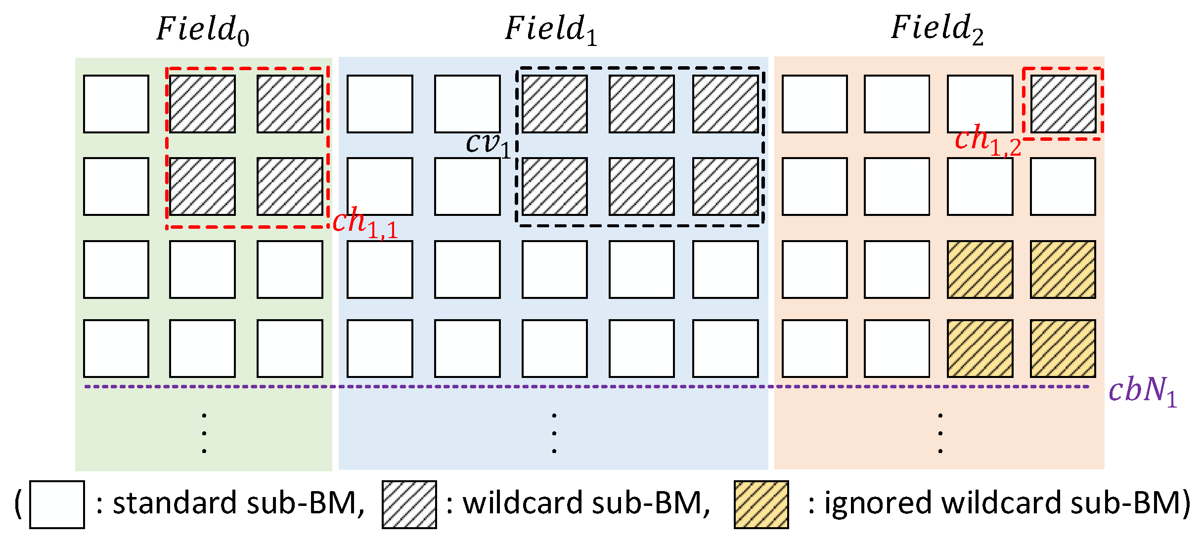
3.2.1. Problem Definition

There are four types of matching in multi-field packet classification: prefix matching, range matching, wildcard matching, and exact matching. Source or destination port field typically require range matching, such as the well-known system port range [0:1023]. To enable hardware to support range matching, a widely used method is range-to-prefix [18]. Prefix matching is typically used for source or destination IP addresses with a subnet mask. Wildcard matching and exact matching can be handled as two particular cases of prefix matching: one matches any value and the other matches only a specific value. Therefore, it is feasible to convert a rule to prefix matching on each matching field. In this paper, we take only prefix matching into consideration.

After transformation, the entire ruleset becomes a Bit-Matrix (BM) with a size of $L\ast N$, as shown in Figure 5. The stride s and cluster n are used to decompose the BM into sub-BMs as introduced before. Each sub-BM will correspond to a BV table as shown in Figure 1. A sub-BM consisting of only wildcards (called wildcard sub-BM) corresponds to the All-1 BV table as shown in Figure 1b. For the stride and cluster of fixed size, the number and location of sub-BMs are also fixed. A different arrangement of the ruleset may result in a different number of wildcard sub-BMs, which may improve the compression percentage. The memory compression problem for BV-based approaches can be defined as follows: Given a BM with decomposition parameters s and n, find an arrangement with the most wildcard sub-BMs that can maximize the compression percentage.

There are altogether $N!$ kinds of permutation schemes for N rules. Given an arrangement of the ruleset, the number of wildcard sub-BMs can be quickly calculated. However, in the worst case, you must traverse $N!$ times to determine the minimum compression percentage, which means the time complexity is $O(N!)$. It can be found that the memory compression problem is equal to classical Traveling Saleman Problem (TSP) [20], which is an NP-hard problem. We propose a heuristic greedy-based algorithm to find the approximate optimal solution in polynomial time, which is named Wildcard-removed Maximum Covering (WeeMC). WeeMC performs the $GreedySearch$ function on a ruleset recursively to give the final arrangement.

3.2.2. Core Function of WeeMC

The pseudo-code of $GreedySearch$ function is shown in Algorithm 1 . For the input ruleset, $GreedySearch$ finds rules that aggregate the largest area of wildcard sub-BMs in the bit-matrix. The search processing takes advantage of the characteristics of prefix matching. Figure 6 shows the distribution of wildcards in two different fields of typical 5-tuple rulesets. Comparing Figure 6a,b, different fields have different numbers of wildcards. Wildcards in prefix matching appear consecutively from the first occurrence to the end. We noticed that the tails of all domains are the most frequently occurring wildcards. Therefore, we split the BM of the ruleset by field and search for the area of wildcard sub-BMs from the end.

Algorithm 1 GreedySearch

Input: The set of fields for searching, $FieldSet$; The set of rules for searching, $RuleSet$; The length of stride, s; The number of cluster, n; Output: The set of remaining fields after searching, $FieldSetElse$; The set of selected rules, $RuleSetFound$; Other helpful extra information, $ResultItem$; 1: for$Fiel{d}_m$ IN $FieldSet$ do 2:     for $p=s$ to $L_m$ do 3:         for $i=1$ to $N_m$ do 4:            if $Rul{e}_{(i,p)}\to Rul{e}_{(i,L_m)}==Wildcards$ then 5:                $N_{p}Array\left[p\right]$$+=1;$ 6:            end if 7:            $Are{a}_{m}Array\left[p\right]$$=p\ast N_{p}Array\left[p\right];$ 8:         end for 9:     end for 10:     $p_m,N_{p_m}\leftarrow MAX\left(Are{a}_{m}Array\right);$ 11:     $Are{a}_{All}Array\left[p_m\right]$$=(p_m\ast N_{p_m})|(s\ast n);$ 12: end for 13: $p_{max},N_{p_{max}}\leftarrow MAX\left(Are{a}_{All}Array\right);$ 14: $FieldSetElse=FieldSet-Fiel{d}_{max};$ 15: if$p_{max}>=s$$and$$N_{p_{max}}>=n$then 16:     $RuleSetFound\leftarrow$$N_{p_{max}}$$rules$$from$$RuleSet;$ 17: else 18:     $RuleSetFound=NULL;$ 19: end if 20: $ResultItem\leftarrow Extra$$Information;$

We use $p_m$ and $N_{p_m}$ to calculate the number of the wildcard sub-BMs covered in $Fiel{d}_m$, $Rul{e}_{(i,p)}\to Rul{e}_{(i,L_m)}$ represents the last $p_m$ bits of a rule in $Fiel{d}_m$ and $N_{p_m}$ is the number of rules that $p_m$ bits are wildcards in $Fiel{d}_m$. Our approach employs a greedy strategy: for a given ruleset and fields, first find the largest combination of $p_m$ and $N_{p_m}$ in each field, and then choose the permutation scheme given by the field with the largest number of coverages. Note that the searching for each field is independent of each other (always through the entire ruleset). In $Fiel{d}_m$, the largest combination of $p_m$ and $N_{p_m}$ satisfies the following conditions:

$$\forall p_i\in \left\{p\right|s\ll p\ll L_m,p\ne p_m\},$$

$$(p_i\ast N_{p_i})|(s\ast n)\ll (p_m\ast N_{p_m})|(s\ast n).$$

$L_m$ indicates the number of bits in $Fiel{d}_m$, s is the stride, and n is the cluster. $RuleSetFound$, one of the results returned by the $GreedySearch$ function, is a sub-ruleset with the maximum number of coverages on $Fiel{d}_{max}$. Line 13 of $GreedySearch$ ensures that at least one wildcard sub-BM is covered in the worst case. The $MAX$ function can be any sorting algorithm that returns the maximum value in $Are{a}_{All}Array$. Here we assume that the $MAX$ function is implemented using a binary search with a time complexity of $O(logn)$. The search time complexity of the $GreedySearch$ function is $O(F\ast (L\ast N+logL)+logF)$. Given a ruleset for multi-field packet classification, N is usually much larger than L and F. Therefore, the time complexity of the $GreedySearch$ function is $O\left(N\right)$.

3.2.3. Combination Searching of WeeMC

The pseudo-code of WeeMC is shown in Algorithm 2. A greedy strategy can quickly find a partial optimal solution, but it is usually not a global optimal solution. After performing the $GreedySearch$ function one time for the entire ruleset, the remaining rulesets can still be optimized. Our scheme performs a combination search of the entire ruleset to obtain an approximate global optimal solution. The $GreedySearch$ function is executed multiple times from the vertical and horizontal directions respectively. The number of searches is called $cbN$ (abbreviation of combination number).

Vertical Search. First perform the $GreedySearch$ function one time on the entire ruleset BM and find $RuleSetNe{w}_v$. The GreedySearch function then continues iteratively on the remaining ruleset (i.e., line 23 of WeeMC). Vertical iterations stop in three cases:

(1)

all rules have been covered;

(2)

no wildcard BM can be found in the remaining rules;

(3)

the number of iterations reaches $cbN$.

Horizontal Search. The $RuleSetNe{w}_v$ is rearranged again after each vertical search. Search for a compressible wildcard sub-BM in a field other than $Fiel{d}_{max}$. The horizontal iteration stops in two cases:

(1)

no wildcard BM can be found in the remaining rules;

(2)

the number of iterations reaches $cbN$.

Figure 7 demonstrates a combination search with $cbN$ = 2. Searching for the sub-ruleset returned by $c{v}_1$ in the vertical direction can obtain 9 wildcard sub-BMs in $Fiel{d}_1$. After the first vertical search, two horizontal searches (by rearranging the sub-rulesets) obtain an additional six wildcard sub-BMs by $c{h}_{1,1}$ in $Fiel{d}_0$ and $c{h}_{1,2}$ in $Fiel{d}_2$, respectively.

Algorithm 2 WeeMC

Input: The set of rules, $DataFile$; The number of combinations, $cbN$; The length of stride, s; The number of cluster, n; Output: An arrangement of the ruleset with maximum compression, $RuleArrangement$; 1: $ALLRuleSet,ALLFieldSet=INIT\left(DataFile\right);$ 2: $RuleSetOL{D}_v,RuleElseSet=ALLRuleSet;$ 3: $FieldSetOl{d}_v=ALLFieldSet;$ 4: for$cv=1$ to $cbN$ do 5:     $FieldSetNe{w}_v,RuleSetNe{w}_v,ResultIte{m}_v=$ 6:     $GreedySearch(FieldSetOl{d}_v,RuleSetOL{D}_v,s,n)$ 7:     if $RuleSetNe{w}_v==NULL$ then 8:         $\mathit{BREAK}$ 9:     end if 10:     $FieldSetOl{d}_h=FieldSetNe{w}_v$ 11:     $RuleSetOL{D}_h=RuleSetNe{w}_v$ 12:     $\mathit{ADD}$$ResultIte{m}_v$ $\mathit{IN}$ $CombResul{t}_h$ 13:     for $ch=1$ to $cbN-1$ do 14:         $FieldSetNe{w}_h,RuleSetNe{w}_h,ResultIte{m}_h=$ 15:         $GreedySearch(FieldSetOl{d}_h,RuleSetOL{D}_h,s,n)$ 16:         if $RuleSetNe{w}_h==NULL$ then 17:            $\mathit{BREAK}$ 18:         end if 19:         $FieldSetOl{d}_h=FieldSetNe{w}_h$ 20:         $RuleSetOL{D}_h=RuleSetNe{w}_h$ 21:         $\mathit{ADD}$ $ResultIte{m}_h$ $\mathit{IN}$ $CombResul{t}_h$ 22:     end for 23:     $RuleSetOL{D}_v=RuleElseSet-RuleSetNe{w}_v$ 24:     if $RuleSetOL{D}_v==NULL$ then 25:         $\mathit{BREAK}$ 26:     end if 27:     $\mathit{ADD}$ $CombResul{t}_h$ $\mathit{IN}$ $CombResul{t}_v$ 28: end for 29: $RuleArrangement\leftarrow$$Extract$$from$$CombResul{t}_v$

3.3. WeeSU Strategy

Dynamic updates are required to support three operations: modification, insertion, and deletion. The Controller component in the standard PE with writable memory is self-reconfigurable. For inserts, the Controller component in the standard PE can convert the new rules into the entire BV table and rewrite the Memory component [15]. In addition, Valid-bit is used to support fast deletion. A modification can be divided into a deletion and an insertion.

The wildcard PEs pose a new challenge for supporting dynamic updates. Modification of the rules may force a wildcard sub-BM to be converted to a standard sub-BM. Correspondingly, there will be a Wildcard PE failure in WeeTP. Although FPGA supports reconfigure wildcard PEs, refactoring all wildcard PEs is prohibitively expensive. To solve this problem, we consider two kinds of updates separately:

(1)

Update bit in standard PE: The Controller component can well support delete, add and modify these three operations.

(2)

Update bit in wildcard PE: The Controller component can still support the delete operation. For inserts and modifications, we use a strategy called Wildcard-removed Sink-Update (WeeSU). For each $cb{N}_j$, the wildcard sub-BMs are congregated above the same field by the greedy strategy. For a bit position, there will always be a standard PE below. Therefore, the insert and modify operations first perform a delete operation in the original location. WeeSU will then search a standard PE with unoccupied location (indexed by valid-bit) and perform an insert operation. Therefore, the sink processing includes a deletion above, a downward searching and a renewedly insertion.

Figure 8 shows an example of the WeeSU. $Sin{k}_1$ indicates that the modified bit of a rule is in the second PE of $Fiel{d}_0$, which is a wildcard PE. $Sin{k}_1$ Delete this rule from the $r_i$th row horizontal pipeline. Then $Sin{k}_1$ looks down to the $r_{(i+1)}$th row to perform the insert operation, assuming that there is a idle position in the corresponding position of the $r_{(i+1)}$th row that can be reused. In the process of $Sin{k}_2$, the $r_i$th row and the $r_{(i+1)}$th row horizontal pipeline have conflicts in $Fiel{d}_1$, and the $r_i$th row and the $r_{(i+2)}$th row horizontal pipeline have conflicts in $Fiel{d}_0$. Therefore, the rule in $Sin{k}_2$ finally sinks from the $r_i$th row to the $r_{(i+3)}$th row.

The sinking strategy ensures that WeeTP still supports dynamic updates while maximizing memory consumption reduction. The saved memory can provide space for inserting new rules. Although this is a common method, we still have to find a better solution for the worst-case update support. In the worst case, the ruleset can be substantially modified in a short period of time. A large number of sinking rules will eventually fill the reserved space of the lowest level horizontal pipeline. To solve this issue, we can utilize the state-of-the-art technology of FPGA, which is called dynamic partial reconfiguration (DPR) [21].

DPR is a common technique to design adaptive and flexible hardware on FPGA. The main idea is to substitute defined regions of programmable logic containing reconfigurable modules at runtime. The partial reconfiguration process takes place without interfering with other parts of the system. Filling the bottommost horizontal pipeline means that at least one horizontal pipeline above is “sparse”, which can be defined as a threshold. Combined with DPR, we can quickly redistribute the rules of the filled underlying pipeline to the different “sparse” pipelines in the upper layers. The state-of-the-art 230 research proves that the dynamic and partial reconfiguration of hardware takes only 10 ms [22], which is acceptable for WeeBV implementation. The time taken for partial reconfiguration is dependent on the FPGA and the size of the region that is reconfigured. Each “sparse” pipeline occupies only a small area and can be quickly reconfigured. Therefore, we believe that DPR technology is acceptable for WeeBV implemention.

4. Optimization Techniques

In order to further increase the compression percentage of WeeTP, we propose optimization techniques MaxPadding and UpstreamRule for two special cases. It should be noted that these two optimization techniques are only fit for some special scenarios. Therefore, these two techniques are optional.

4.1. MaxPadding Technique

In multiple horizontal searches, the greedy strategy ignores the suboptimal compression scheme and only the optimal solution is selected. However, the discarded suboptimal choice might lead to the overall optimality. When the ruleset presents obvious local aggregation, the optimal solution and the suboptimal solution found by greedy strategy are usually close to each other. In this case, the wildcard sub-BMs are ignored in many suboptimal solutions. To solve this issue, we propose a method called MaxPadding. After each horizontal search, we compare the size of the $RuleSetNe{w}_h$ and the $RuleSetOl{d}_h$. If the $FieldSetNe{w}_h$ is not greater than $\frac{2}{3}$ (which is a threshold from experience) of $RuleSetOl{d}_h$, we consider that there is a suboptimal solution that cannot be ignored as shown in Figure 9. In the rules that $RuleSetOl{d}_h$ subtracts $RuleSetNe{w}_h$, MaxPadding continues to perform a horizontal search. The number of searches is $MIN$($LEN$($FieldSetOl{d}_h$), $cbN-1$). Normally, $cbN$ will be larger than $LEN\left(FieldSetOl{d}_h\right)$.

MaxPadding technology is helpful for some types of rulesets. MaxPadding technique appropriately may increase the total search time overhead. Our experience has shown that MaxPadding technique can reduce 37.42% memory consumption for $F{W}_4$ rulesets while increasing search time by 2 to 3 times. The trade-off between search time and promotion effects should be considered.

4.2. UpstreamRule Technique

In order to calculate the maximum compression effect corresponding to $p_m$, the greedy strategy will also include some rules with wildcard suffixes longer than $p_m$. These wildcard bits larger than $p_m$ will eventually be ignored, which are shown in Figure 10. To solve this issue, we propose a technique called UpstreamRule. It is assumed that the fields selected in the horizontal direction for c times are $Fiel{d}_{m1}$ to $Fiel{d}_{mc}$, and the number of corresponding rules is $N_{p_{m1}}$ to $N_{p_{mc}}$, respectively. The reverse order check is performed from $Fiel{d}_{mc}$, and the rules in which the wildcard length exceeds $p_{mc}$ in the $N_{p_{mc}}$ rules are arranged in descending order of the length of the wildcards. These wildcards beyond $p_{mc}$ then overlap as many wildcard BMs as possible.

The purpose of arranging from large to small is to ensure the correctness of dynamic updates. UpstreamRule technique presents a challenge to the Sink-Update policy. In a horizontal pipeline, more wildcard PEs may have a greater chance of update failure. A modified rule may need to sink more horizontal pipelines. As an option, we recommend using UpstreamRule technology with fewer dynamic updates.

5. Evaluation

5.1. Experimental Setup

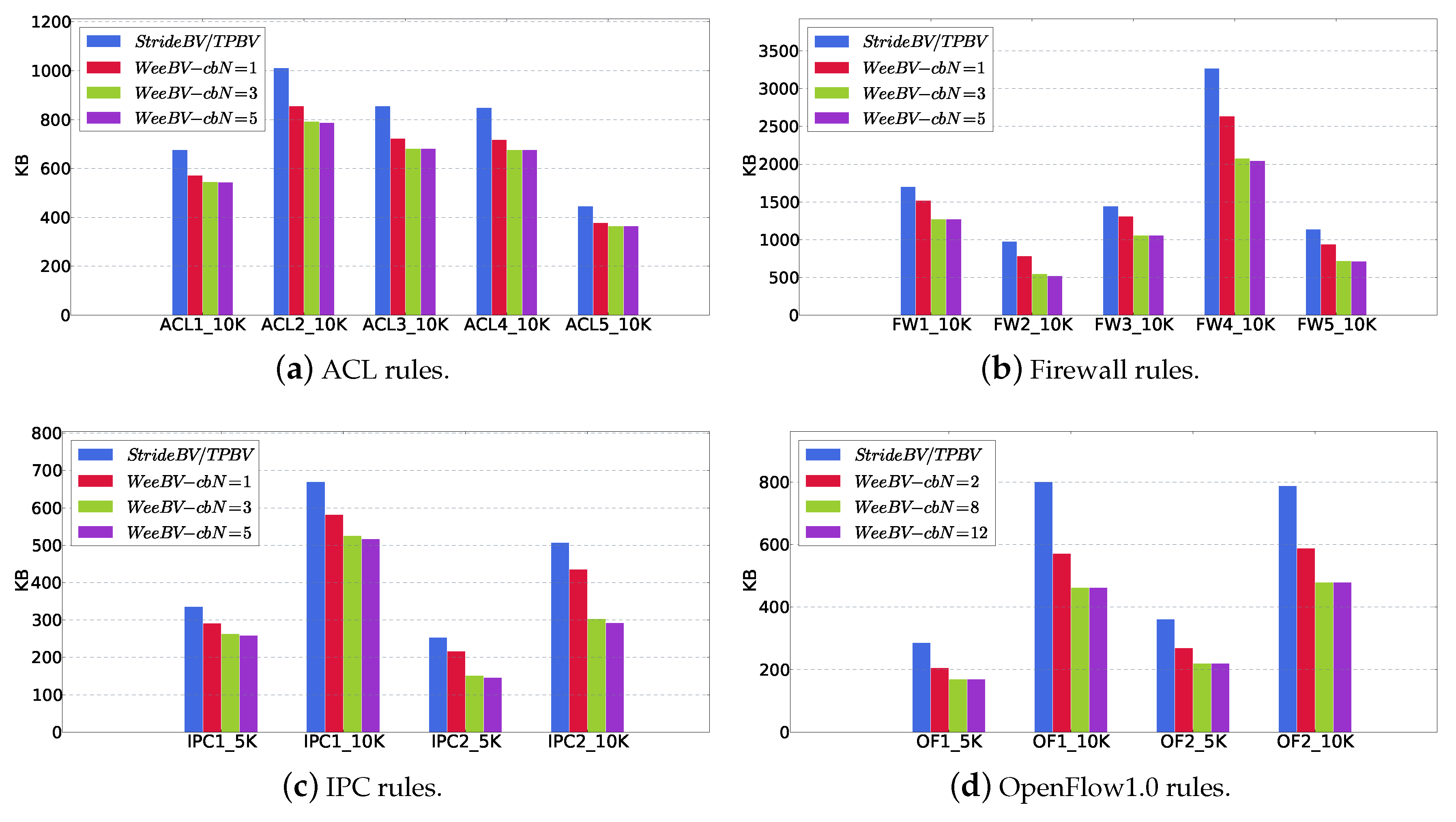
Synthetic classifiers: To test the performance of our scheme and prior art, we generate the 5-tuple rules with real parameters by the well-known ClassBench [16]. In our experiments, the 5-tuple rules we have used contain Accesses Control List (ACL), Firewall (FW) and IP Chain (IPC). The seed file which ClassBench provided from real-life 5-tuple rules can make the performance as close to practice as possible. Besides, we used the OpenFlow1.0 rules from a data-center generated by the ClassBench-ng [17], which is an excellent tool inherited from ClassBench.

Implementation platform: We verify the WeeTP with an Intel${}^{\circledR }$ STRATIX V GS 5SGSD5 FPGA, which contains 39Mb Block RAM, 172,600 Adaptive Logic Modules (ALMs) and 690,400 registers. Limited to the experimental platform, we use simulation software to test performance. Simulation is also widely used in other high-level conferences and companies. WeeMC algorithm and optimization techniques are run on a machine with Intel Xeon E5-3650 CPU and Ubuntu 16.04 LTS operation system. More details and source codes are available at Github [23].

5.2. cbN for WeeMC

We compare our scheme WeeBV with the widely used algorithm: StrideBV. The StrideBV is the de facto implementation for BV-based approaches. In fact, the majority of onchip memory of FPGAs is organized in blocks. For example, the minimum size block memory on STRATIX V GS FPGAs is 20 Kb, programmable from 20 K × 1 bit to 512 × 40 bits [24]. In other words, the minimum memory depth is 512, which requires the address width be at least 9 bits. Even though the theoretical BV table occupation of FSBV is $O(2L\ast N)$, each bit of the matching field will occupy a block memory in the implementation, which leads to a great waste of actual memory. The Two-dimensional Pipelined BV-based algorithm (TPBV) in the state-of-the-art research [15] has the same memory consumption of bit-vectors as StrideBV. According to Equation (1), the parameter n of the TPBV cannot affect the memory consumption of the BV tables. Lots of homogeneous PE in TPBV can consume additional logical resources. Given the inconsistencies between our own implementation of PE and the details in the original, we only compare the memory footprint of the BV tables. We choose the parameter s to be 4 and n to be 8, which is the best solution in [15].

Figure 11 shows the compression effect on the four type rulesets—up to 22%, 47%, 42% and 41% for ACL, FW, IPC, and OpenFlow, respectively. When $cbN$ is equal to the number of matching fields, WeeMC searches in each field to achieve maximum compression. The iterative result is approximated by iterating three times for the 5-tuple rulesets. This is because most rules retain at least two fields that are exactly matched. The best compression percentages for different types of rulesets are also different because the proportion of wildcards in the ruleset with different features appears differently. The FW ruleset usually only cares about the combination of two fields of a source or destination IP address and port, so the compression ratio is the largest in the 5-tuple rulesets. The compression percentages of the Open flow rulesets are also high, since most rules only use 3–4 fields of 12 matching fields.

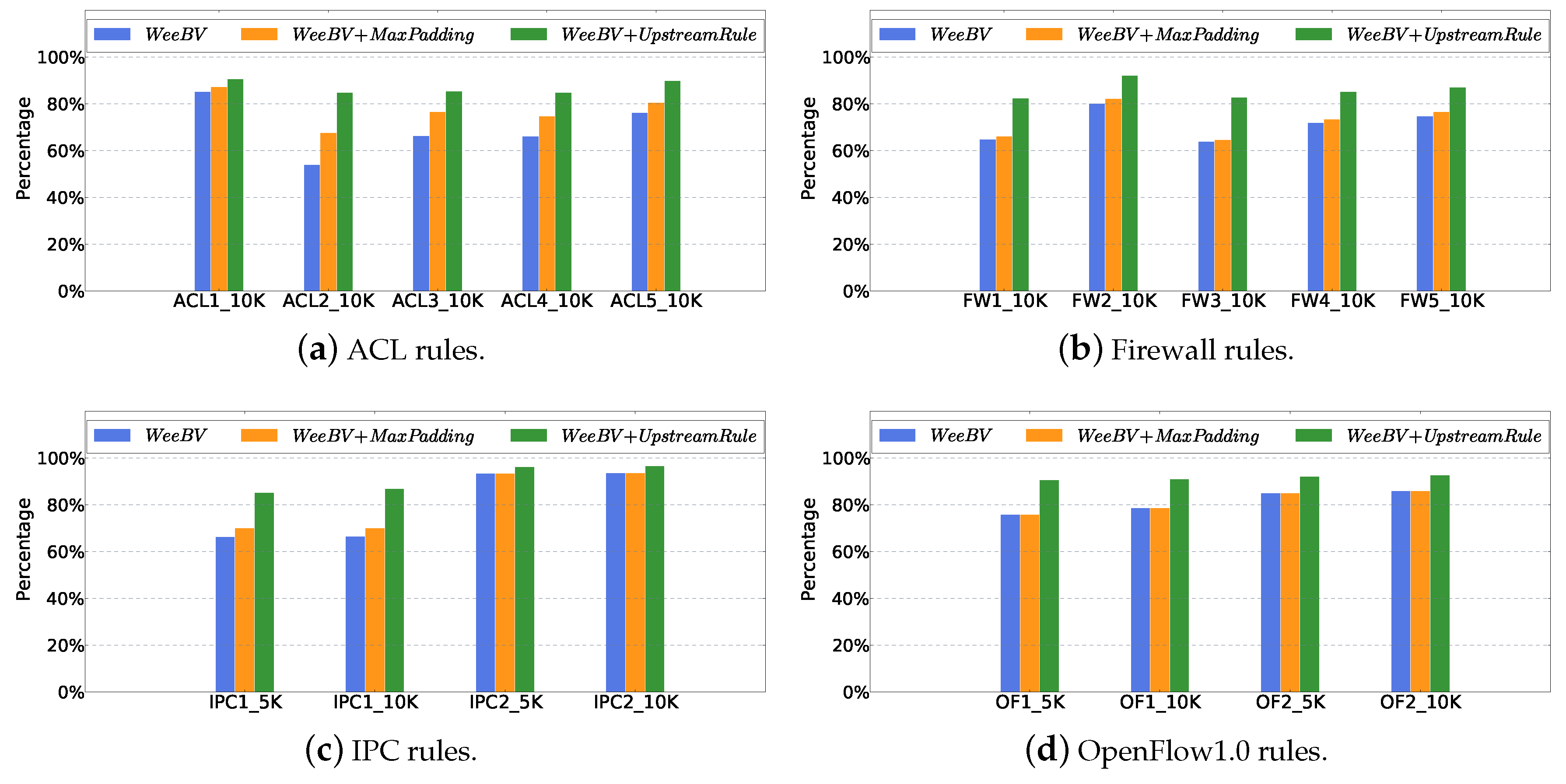
5.3. Compression with MaxPadding and UpstreamRule

Since different types of rulesets have different characteristics, the number of wildcards that can be compressed in the bit matrix transformed from the ruleset is also different. When the parameters s and n are not equal to 1, the wildcards in the bit matrix cannot all be compressed. In this case, there is a supremum of the compression percentage for the different arrangement schemes, which is named $MaxCompressed$. $MaxCompressed=\frac{Coun{t}_w}{L\ast N}$, and $Coun{t}_w$ is the total number of wildcards in the ruleset. Figure 2 shows the $MaxCompressed$ for each ruleset. It can be observed that the average $MaxCompressed$ of OpenFlow is the largest, more than 40% in Figure 2. In other words, we can also measure memory compression as a percentage of $MaxCompressed$.

We show the memory compression of the WeeMC algorithm and its optimization techniques in Figure 12. MaxPadding has a significant memory compression increase for the ACL ruleset in Figure 12a. This is because rules in the ACL ruleset typically aggregate heavily in the source IP address field and the destination IP address field. These massive aggregations leave space for optimization in MaxPadding. Interestingly, MaxPadding does not help the OpenFlow ruleset in Figure 12d. We think this is related to the rule strategy in a certain data center. Note that for all types of rule sets, UpstreamRule improves the WeeMC algorithm to varying degrees. Our solution can eventually activate 80% of MaxCompressed for all types of rulesets. The UpstreamRule technique helps the WeeMC algorithm get closer to the globally optimal solution.

5.4. Resource and Throughput

Multiple metrics can be used to select parameters s and n, such as throughput, latency, and memory consumption. Our goal is to verify the impact of reducing the memory consumption of wildcards on throughput. To maximize memory utilization, we use $s=9$ and $n=40$ to achieve state-of-the-art research (TPBV) and WeeBV, respectively. That is because the size of the Block Memory of the used FPGA is m20K, which is equal to $20\times 1024=40\times 2^9$.

Table 1. Resource consumption and performance of WeeBV and TPBV ${}^{\dotplus }$ for $s=9$ and $n=40$.

RuleSet Type	Rule Number	Block Memory		ALMs		Registers		Clock Rate
		(KB)		Number		Number		(MHz)
		TPBV	WeeBV	TPBV	WeeBV	TPBV	WeeBV	TPBV	WeeBV
ACL	128	120	95	2690	2126	4221	3335	160.03	153.66
	256	210	166	4492	3549	7085	5598	155.45	149.95
	512	390	309	8015	6332	12,607	9960	151.54	142.80
	1024	780	617	15,605	12,328	24,470	19,332	145.33	138.25
FW	128	120	65	2690	1453	4221	2280	160.03	153.13
	256	210	114	4492	2426	7085	3826	155.45	149.43
	512	390	211	8015	4329	12,607	6808	151.54	140.68
	1024	780	422	15,605	8427	24,470	13,214	145.33	136.41
IPC	128	120	71	2690	1588	4221	2491	160.03	153.36
	256	210	124	4492	2651	7085	4181	155.45	149.38
	512	390	231	8015	4729	12,607	7439	151.54	141.29
	1024	780	461	15,605	9207	24,470	14,438	145.33	136.29
OpenFlow1.0	128	320	192	5684	3411	8202	4922	153.14	149.28
	256	560	336	9635	5782	13,860	8316	151.58	147.38
	512	1040	624	17,537	10,523	25,176	15106	150.2	145.67
	1024	2080	1248	34,658	20,795	49,694	29,817	147.71	144.01

∔ Two-dimensional Pipelined BV-based algorithm in [15].

shows the resource consumption and performance of TPBV and WeeBV for different sizes and types of rulesets. We use the Clock Rate to reflect throughput. Note that we tested the Clock Rate of a simple prototype system, which contains not only the packet classification module but also the parser module. Since we did not optimize the parameters s and n for throughput, the Clock Rate does not represent the maximum performance of the system. For different types of 5-tuple rulesets with the same size, the resource consumption of the TPBV is equivalent. The traditional BV-based approach is ruleset-feature independent. Each type of ruleset uses all of the seed files of this type to generate a different number of rules. The resource consumption reduced by WeeBV in Table 1 is consistent with the experimental results in section V.B. For rulesets of the same type and size, WeeBV does not have significant damage throughput compared to the TPBV in state-of-the-art research. In addition, the OpenFlow1.0 rulesets consume more resources and require more complex processing due to the increased matching length, thus degrading performance. The wildcard PEs also reduce the number of memory accesses, which will lower local latency and power consumption.

6. Related Works

A rule is an individual predefined entry used for classifying a packet, which is associated with a unique rule ID (RID), a priority and an action. Multi-field packet classification can be defined as: Given a ruleset of size N and an input packet header that consists of F fields, find all the rules matching the packet header and export the RID of the highest priority rule.

Current packet classifications can be classified into two main categories: algorithmic solutions (usually using RAM) and Ternary Content Addressable Memory (TCAM)-based solutions [25,26]. Each storage unit in TCAM can have three different types of states: {0, 1, and *}, and TCAM can search all rules in parallel in a single lookup cycle. TCAM suffers high cost and high power consumption, and hard to perform range matching [26]. Anat Bremler-Barr et al. proposed gray code [27] and layered interval code [28] to enable TCAM support range matching at the cost of entry explosion. Thus in practice, the number of range fields is severely limited.

Decision-tree-based approaches [4,5] analyze all fields in a ruleset to construct decision trees for packet classification. Decision-tree-based solutions traverse the tree by using individual field values to make branching decisions at each node until a leaf is reached. Tree depth and rule duplication in a decision tree affect the searching efficiency and memory requirement of one implementation. Both of them increase with the growth of field numbers which results in an exponential increase of memory requirement and increasing processing latency.

Tuple space solutions [3,6] are usually software-based and they leverage the fact that the number of distinct tuples is much less than that of rules in a ruleset. A tuple defines the number of significant bits in a prefix match field, the nesting level and range ID of a range field, and the existence of a value for an exact match field in a ruleset. Tuple-space-based solutions efficiently compress a ruleset by storing those valid bits of each field only. Besides, tuple-space-based solutions perform the search of each tuple independently and take advantage of parallelism. With the growth field number in a ruleset, both tuple number and tuple size increase. A longer processing latency could be expected.

Decomposition-based approaches [12,29] first search each packet header field individually. The partial results are then merged to produce the final result. Bit-vector-based schemes [13,14,15] are detailed earlier. Due to the limited hardware resources, they cannot support the growing rulesets. The rapidly increasing matching fields consume memory resources dramatically.

7. Conclusions

In this paper, we present a memory-,optimized scheme named WeeBV to support a massive set of rules while ensuring high throughput processing performance. WeeBV first constructs a heterogeneous two-dimensional lookup pipeline called WeeTP. WeeTP processes each BV table by a modular PE arranged in the two-dimensional array. In addition, WeeTP distinguishes PEs into standard PEs and wildcard PEs. The wildcard PEs reduce Memory component and the n-bit and logic unit for saving memory resource. The WeeBV utilizes a greedy algorithm named WeeMC, which is used to maximize the compression of the WeeTP by rearranging the ruleset. An update strategy called Sink-Update is proposed to support real-time dynamic updates. Looking forward, we propose optimization techniques MaxPadding and UpstreamRule for two special cases. Experimental results show that WeeTP has an excellent compression effect on both 5-tuple and OpenFlow rulesets.

References

1. ONF. OpenFlow Switch Specification. Available online: https://www.opennetworking.org/software-defined-standards/specifications/ (accessed on 8 October 2019).
2. McKeown, N.; Anderson, T.; Balakrishnan, H.; Parulkar, G.M.; Peterson, L.L.; Rexford, J.; Shenker, S.; Turner, J.S. OpenFlow: Enabling innovation in campus networks. SIGCOMM Comput. Commun. Rev. 2008, 38, 69–74. [Google Scholar] [CrossRef]
3. Pfaff, B.; Pettit, J.; Koponen, T.; Jackson, E.J.; Zhou, A.; Rajahalme, J.; Gross, J.; Wang, A.; Stringer, J.; Shelar, P.; et al. The Design and Implementation of Open vSwitch. In Proceedings of the 12th USENIX Symposium on Networked Systems Design and Implementation (NSDI ’15), Oakland, CA, USA, 4–6 May 2015; pp. 117–130. [Google Scholar]
4. Singh, S.; Baboescu, F.; Varghese, G.; Wang, J. Packet classification using multidimensional cutting. In Proceedings of the ACM SIGCOMM 2003 Conference on Applications, Technologies, Architectures, and Protocols for Computer Communication, Karlsruhe, Germany, 25–29 August 2003; pp. 213–224. [Google Scholar] [CrossRef]
5. Vamanan, B.; Voskuilen, G.; Vijaykumar, T.N. EffiCuts: Optimizing packet classification for memory and throughput. In Proceedings of the ACM SIGCOMM 2010 Conference on Applications, Technologies, Architectures, and Protocols for Computer Communications, New Delhi, India, 30 August–3 September 2010; pp. 207–218. [Google Scholar] [CrossRef]
6. Srinivasan, V.; Suri, S.; Varghese, G. Packet Classification Using Tuple Space Search. In Proceedings of the SIGCOMM ’99 Conference on Applications, Technologies, Architectures, and Protocols for Computer Communication, Cambridge, MA, USA, 30 August–3 September 1999; pp. 135–146. [Google Scholar] [CrossRef]
7. Lakshminarayanan, K.; Rangarajan, A.; Venkatachary, S. Algorithms for advanced packet classification with ternary CAMs. In Proceedings of the ACM SIGCOMM 2005 Conference on Applications, Technologies, Architectures, and Protocols for Computer Communications, Philadelphia, PA, USA, 22–26 August 2005; pp. 193–204. [Google Scholar] [CrossRef]
8. Ma, Y.; Banerjee, S. A smart pre-classifier to reduce power consumption of TCAMs for multi-dimensional packet classification. In Proceedings of the ACM SIGCOMM 2012 Conference, Helsinki, Finland, 13–17 August 2012; pp. 335–346. [Google Scholar] [CrossRef]
9. Li, B.; Tan, K.; Luo, L.L.; Peng, Y.; Luo, R.; Xu, N.; Xiong, Y.; Cheng, P. ClickNP: Highly flexible and High-performance Network Processing with Reconfigurable Hardware. In Proceedings of the ACM SIGCOMM 2016 Conference, Florianopolis, Brazil, 22–26 August 2016; pp. 1–14. [Google Scholar] [CrossRef]
10. Fu, W.; Li, T.; Sun, Z. FAS: Using FPGA to Accelerate and Secure SDN Software Switches. Secur. Commun. Netw. 2018, 2018, 5650205. [Google Scholar] [CrossRef]
11. Zhao, T.; Li, T.; Han, B.; Sun, Z.; Huang, J. Design and implementation of Software Defined Hardware Counters for SDN. Comput. Netw. 2016, 102, 129–144. [Google Scholar] [CrossRef]
12. Lakshman, T.V.; Stiliadis, D. High-Speed Policy-Based Packet Forwarding Using Efficient Multi-Dimensional Range Matching. In Proceedings of the ACM SIGCOMM ’98 Conference on Applications, Technologies, Architectures, and Protocols for Computer Communication, Vancouver, BC, Canada, 31 August–4 September 1998; pp. 203–214. [Google Scholar] [CrossRef]
13. Jiang, W.; Prasanna, V.K. Field-split parallel architecture for high performance multi-match packet classification using FPGAs. In Proceedings of the SPAA 2009: 21st Annual ACM Symposium on Parallelism in Algorithms and Architectures, Calgary, AB, Canada, 11–13 August 2009; pp. 188–196. [Google Scholar] [CrossRef]
14. Ganegedara, T.; Jiang, W.; Prasanna, V.K. A Scalable and Modular Architecture for High-Performance Packet Classification. IEEE Trans. Parallel Distrib. Syst. 2014, 25, 1135–1144. [Google Scholar] [CrossRef]
15. Qu, Y.R.; Prasanna, V.K. High-Performance and Dynamically Updatable Packet Classification Engine on FPGA. IEEE Trans. Parallel Distrib. Syst. 2016, 27, 197–209. [Google Scholar] [CrossRef]
16. Taylor, D.E.; Turner, J.S. ClassBench: A packet classification benchmark. IEEE/ACM Trans. Netw. 2007, 15, 499–511. [Google Scholar] [CrossRef]
17. Matouvsek, J.; Antichi, G.; Lucansky, A.; Moore, A.W.; Korenek, J. ClassBench-ng: Recasting ClassBench after a Decade of Network Evolution. In Proceedings of the ACM/IEEE Symposium on Architectures for Networking and Communications Systems (ANCS 2017), Beijing, China, 18–19 May 2017; pp. 204–216. [Google Scholar] [CrossRef]
18. Kogan, K.; Nikolenko, S.I.; Rottenstreich, O.; Culhane, W.; Eugster, P. SAX-PAC (Scalable And eXpressive PAcket Classification). In Proceedings of the ACM SIGCOMM 2014 Conference, Chicago, IL, USA, 17–22 August 2014; pp. 15–26. [Google Scholar] [CrossRef]
19. Hsieh, C.; Weng, N. Many-Field Packet Classification for Software-Defined Networking Switches. In Proceedings of the 2016 Symposium on Architectures for Networking and Communications Systems (ANCS 2016), Santa Clara, CA, USA, 17–18 March 2016; pp. 13–24. [Google Scholar] [CrossRef]
20. Dantzig, G.B.; Fulkerson, D.R.; Johnson, S.M. Solution of a Large-Scale Traveling-Salesman Problem. Oper. Res. 1954, 2, 393–410. [Google Scholar] [CrossRef]
21. Abel, N. Design and Implementation of an Object-Oriented Framework for Dynamic Partial Reconfiguration. In Proceedings of the International Conference on Field Programmable Logic and Applications (FPL 2010), Milano, Italy, 31 August–2 September 2010; pp. 240–243. [Google Scholar] [CrossRef]
22. Kalb, T.; Göhringer, D. Enabling dynamic and partial reconfiguration in Xilinx SDSoC. In Proceedings of the International Conference on ReConFigurable Computing and FPGAs (ReConFig 2016), Cancun, Mexico, 30 November–2 December 2016; pp. 1–7. [Google Scholar] [CrossRef]
23. Li, C. Open-Source of WeeBV Prototypeon on FPGA. Available online: https://github.com/LCLinVictory/WeeBV (accessed on 8 October 2019).
24. Intel. Intel STRATIX V GS FPGAs. Available online: https://www.intel.com/content/dam/www/programmable/us/en/pdfs/literature/pt/stratix-v-product-table.pdf (accessed on 8 October 2019).
25. Taylor, D.E. Survey and taxonomy of packet classification techniques. ACM Comput. Surv. 2005, 37, 238–275. [Google Scholar] [CrossRef] [Green Version]
26. Yang, T.; Liu, A.X.; Shen, Y.; Fu, Q.; Li, D.; Li, X. Fast OpenFlow Table Lookup with Fast Update. In Proceedings of the 2018 IEEE Conference on Computer Communications (INFOCOM 2018), Honolulu, HI, USA, 16–19 April 2018; pp. 2636–2644. [Google Scholar] [CrossRef]
27. Bremler-Barr, A.; Hendler, D. Space-Efficient TCAM-Based Classification Using Gray Coding. IEEE Trans. Comput. 2012, 61, 18–30. [Google Scholar] [CrossRef]
28. Bremler-Barr, A.; Hay, D.; Hendler, D. Layered interval codes for TCAM-based classification. Comput. Netw. 2012, 56, 3023–3039. [Google Scholar] [CrossRef] [Green Version]
29. Baboescu, F.; Varghese, G. Scalable Packet Classification. In Proceedings of the 2001 Conference on Applications, Technologies, Architectures, and Protocols for Computer Communications (SIGCOMM ’01), San Diego, CA, USA, 27–31 August 2001; pp. 199–210. [Google Scholar] [CrossRef]
Figure 1. A matching example for a 4-bit ruleset with s = 2 and n = 3.
Electronics 08 01159 g001
Figure 2. Percentages of wildcards in typical rulesets.
Electronics 08 01159 g002
Figure 3. Architecture of WeeTP for Figure 1b.
Electronics 08 01159 g003
Figure 4. Stardard PE vs. Wildcard PE.
Electronics 08 01159 g004
Figure 5. Example of sub-Bit-Matrix (BM) in bit-matrix of a ruleset.
Electronics 08 01159 g005
Figure 6. Wildcards distribution in two different fields of typical rulesets.
Electronics 08 01159 g006
Figure 7. Example of sub-BMs to be removed with c b N = 2 .
Electronics 08 01159 g007
Figure 8. Sinking operations of WeeSU.
Electronics 08 01159 g008
Figure 9. An example can apply MaxPadding with c b N = 2 .
Electronics 08 01159 g009
Figure 10. An example can apply UpstreamRule with c b N = 1 .
Electronics 08 01159 g010
Figure 11. Memory consumption of bit-vectors for the different rulesets.
Electronics 08 01159 g011
Figure 12. Normalized memory consumption relative to Maxcompressed.
Electronics 08 01159 g012