An Inverse Vehicle Model for a Neural-Network-Based Integrated Lateral and Longitudinal Automatic Parking Controller

Abstract

The majority of currently used automatic parking systems exploit the planning-and-tracking approach that involves planning the reference trajectory first and then tracking the desired reference trajectory. However, the response delay of longitudinal velocity prevents the parking controller from tracing the desired trajectory because the vehicle’s velocity and other state parameters are not synchronized, while the controller maneuvers the vehicle according to the planned desired velocity and steering profiles. We propose an inverse vehicle model to provide a neural-network-based integrated lateral and longitudinal automatic parking controller. We approximated the relationship of the planned velocity to the vehicle’s velocity using a second-order difference equation that involves the response characteristic of the vehicle’s longitudinal delay. The adjusted desired velocity to track the origin-planned velocity is calculated using the inverse vehicle model. Furthermore, we proposed an integrated longitudinal and lateral parking controller using an artificial neural network (ANN) model trained on a dataset applying the inverse vehicle model. By learning the control laws between the vehicle’s states and the corresponding actions, the proposed ANN-based controller could yield a steering angle and the adjusted desired velocity to complete automatic parking in a confined space.

1. Introduction

Several studies to develop automatic parking systems have been conducted, from recognizing vacant parking spaces [1] to booking parking lots using blockchain [2]. Despite much pioneering prior work, the automatic parking control of a car in a tiny space remains a problem to be resolved in the implementation of advanced driver assistant systems or autonomous vehicles. Most conventional automatic parking controllers exploit a step-by-step approach that involves planning the reference trajectory first and then tracking the desired reference trajectory to move the car to the destination. These parking controllers employ a feedback control loop to track the reference path/trajectory within an allowable error tolerance. The reference trajectory planning methods can be classified into the following two groups: The geometric planning and mathematical optimization approaches. In the geometric planning methods, some form of curves such as β-spline [3], Bézier [4,5], clothoid [6], or polynomial curves [7,8] are generated as a set of reference trajectories. The mathematical optimization approaches, firstly formulating a cost function of the automatic parking problem and then minimizing the objective cost function [9,10,11,12,13]. Besides car-like vehicles, reference trajectory is feasible in the case of parking N-trailer vehicles when complicated kinematic constraints are taken into account in planning the trajectory [14,15,16].

Fuzzy-based and knowledge-based approaches have been presented [17,18,19]. These methods are capable of providing solutions within a range of designed rules with an advantage in easy implements and practical usages.

Recently, methods based on deep neural networks have been expected to solve the drawbacks of the mentioned step-by-step approaches by maneuvering vehicles without prior offline trajectory planning [20,21,22,23]. By training an artificial neural network (ANN) using a dataset generated by simulation or experiment, the ANN learns hyper-dimensional relationships between the current vehicle states and the appropriate vehicle maneuvering signals. Instead of calculating the parking trajectory offline, the ANN-based parking controller can yield a direct maneuvering signal of the steering angle and velocity online, while the vehicle is moving into a parking space. Liu et al. presented a method to enumerate all the possible parking trajectories and corresponding steering actions, and then have the parking controller learn the relationship between the given initial-and-final state pairs and the corresponding sequence of steering actions using an ANN [20]. Li et al. proposed an end-to-end neural-network-based automatic parking controller [21]. Rathour also proposed an encoder-decoder architecture for automatic parking [22]. Moon et al. developed an automatic parking controller with a twin ANN architectures [23].

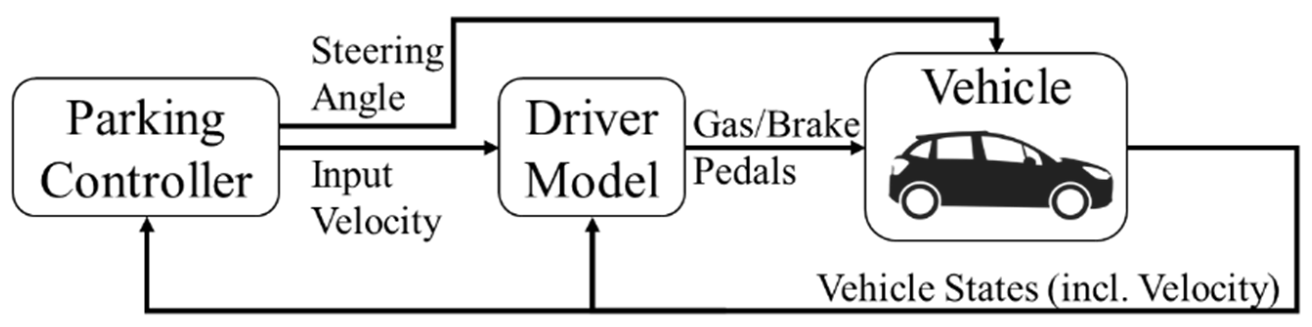
However, neither the planning-based methods nor ANN-based controllers have taken account of longitudinal control delay for a vehicle under automatic parking. Figure 1 shows a typical block diagram of a conventional automatic parking controller. The driver model is a controller that converts the input velocity into the desired positions of gas and brake pedals, that is, the maneuvering input for the vehicle’s longitudinal velocity control. In planning-and-tracking methods, the parking controller maneuvers according to a predetermined trajectory as the reference path. Meanwhile, in ANN-based methods, the parking controller is trained using various deep learning techniques [20,21,22,23]. Longitudinal latency, the delay time between the input velocity and the real velocity of the vehicle, is unavoidable in vehicle dynamics control. Because the parking controller has an architecture of integrated lateral and longitudinal control, the latency of longitudinal velocity causes a mismatch in temporal synchronization between the steering angle signal and desired vehicle velocity (i.e. the control input of the gas and brake pedals).

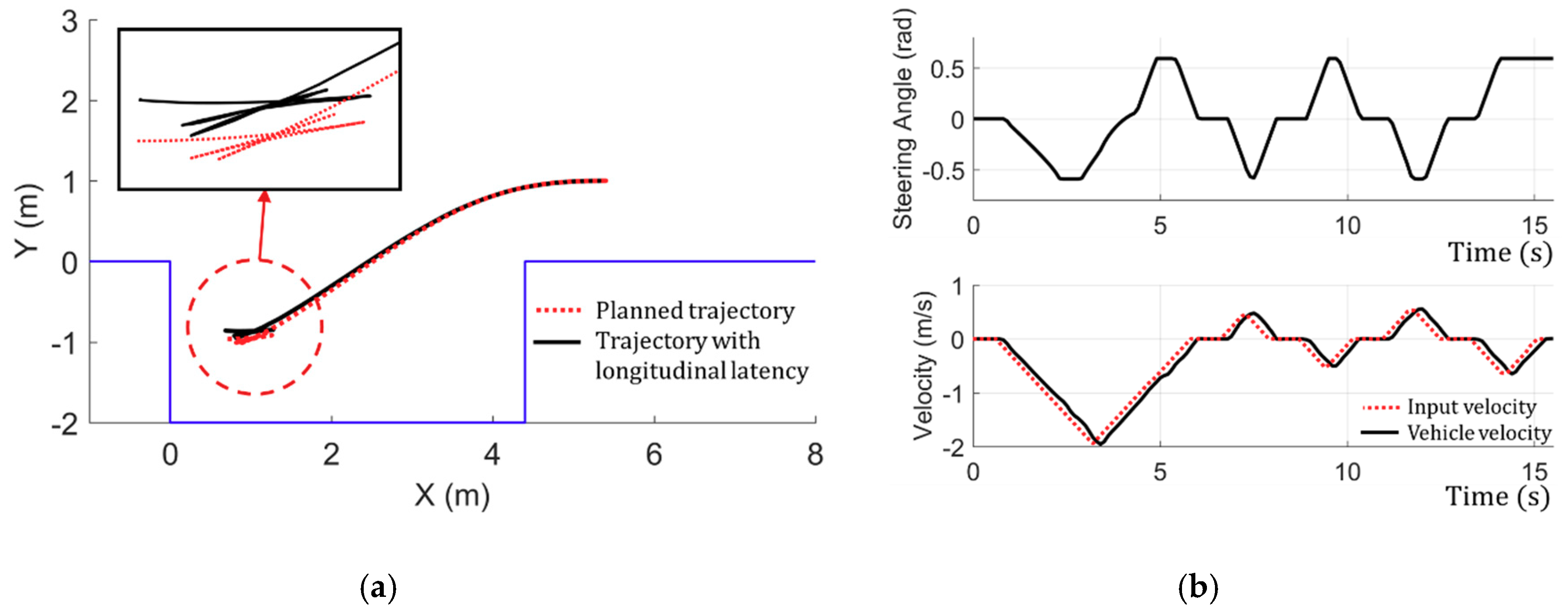
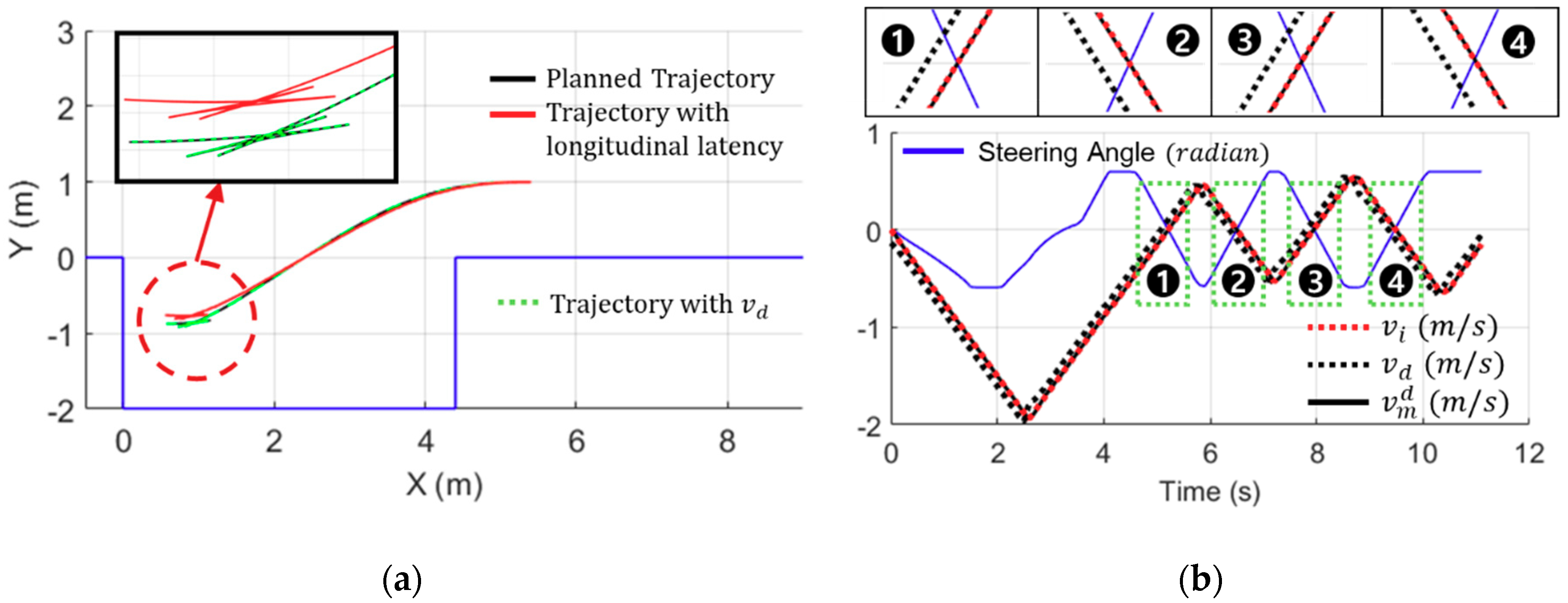
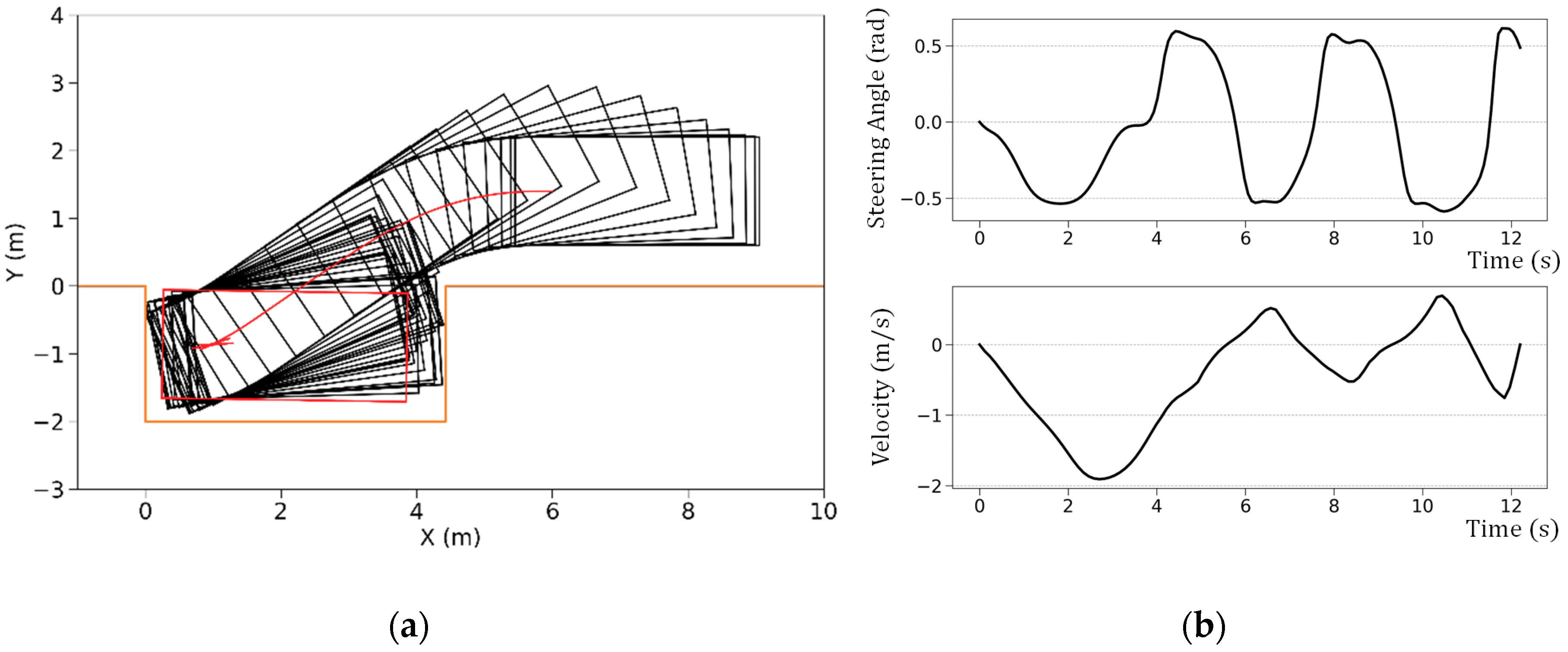
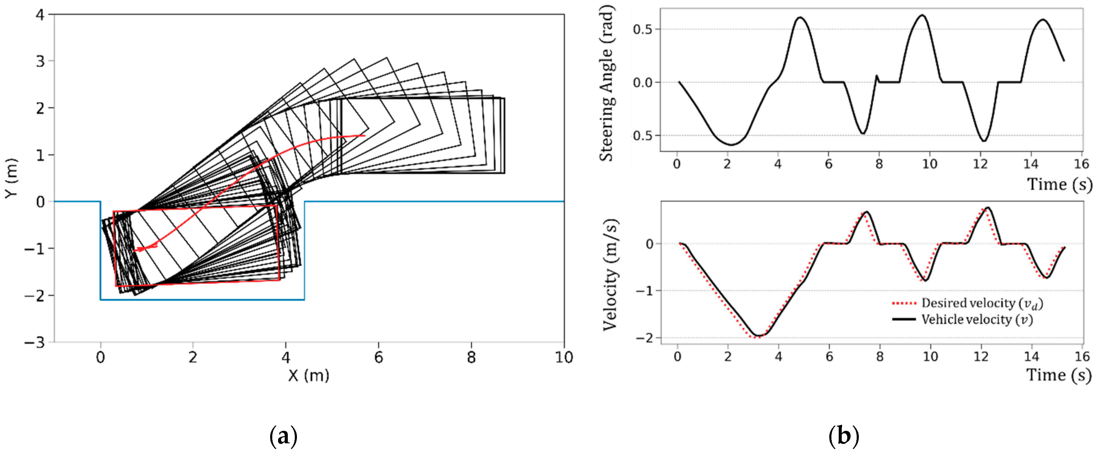
Figure 2 shows a simulated example of a conventional automatic parking control system using the optimal reference planning method [13] that does not regard the latency of longitudinal response. The simulated trajectory deviates from that of the planned reference, as shown in Figure 2a. The simulated result shows that the vehicle’s velocity has a delay from the desired input velocity of the parking controller; consequently, this delay, shown in Figure 2b, causes an out-of-temporal synchronization between the reference steering angle and longitudinal velocity control, which need to match for integrated lateral and longitudinal control. The mismatch of the temporal synchronization between the velocity and steering control signals brought by longitudinal latency eventually leads to a discrepancy between the planned and actual trajectories, making precise automatic parking control in a confined space difficult.

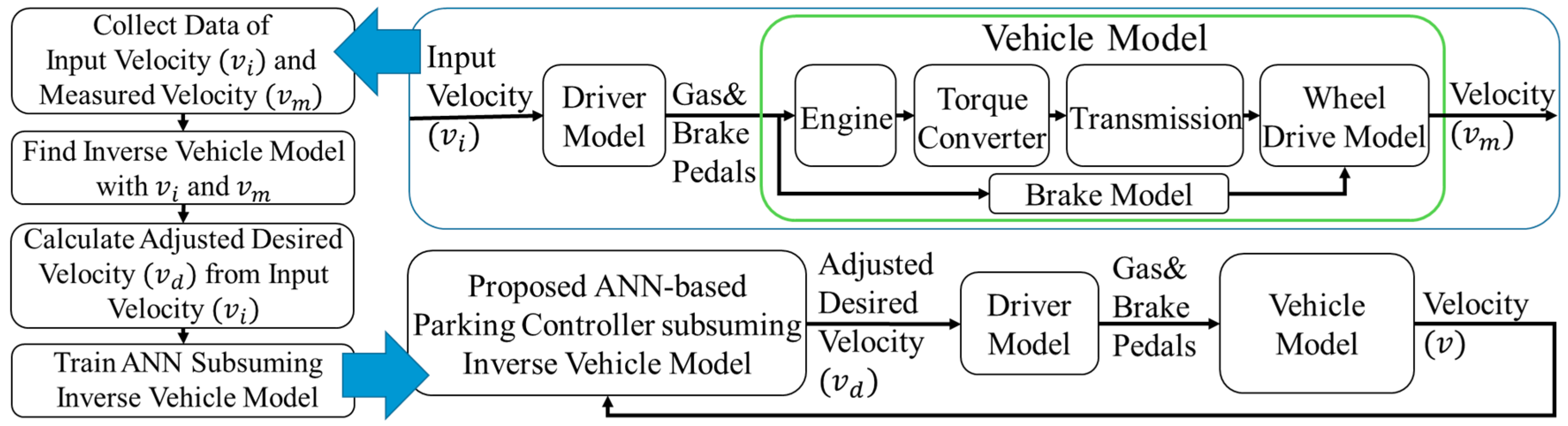
To overcome the mentioned problem caused by the latency of longitudinal response, we propose an inverse vehicle longitudinal velocity model that estimates the desired input velocity required to track the reference trajectory by canceling the effective response delay time from the input demand to longitudinal velocity. We attempt to verify that the inverse vehicle model is applicable to ANN-based automatic parking controllers without loss of synchronization between the lateral and longitudinal control signals to complete automatic parking in confined spaces.

This paper is organized into five sections. Section 2 explains how to model the relationship between the planned input and vehicle velocities. Section 3 describes how to solve the parallel parking problem, how to generate a training dataset for learning parking maneuvers, and the proposed automatic parking controller that is based on an ANN. Simulation results and discussions are presented in Section 4. Finally, the conclusions are drawn in Section 5.

2. Concept and Derivation of the Proposed Inverse Vehicle Model

2.1. Modeling Vehicle Longitudinal Dynamics Using the Inverse Vehicle Model

Figure 3 shows the proposed steps and procedure for developing the inverse vehicle model for the neural network-based parking controller. The longitudinal speed control system of the subject vehicle adopted in this research consists of a driver model and a vehicle dynamics model describing the longitudinal speed control [24], as shown in Figure 3. The vehicle dynamics model representing the dynamic properties of the longitudinal velocity control consists of an engine, a transmission system with a torque converter, and a wheel drive model. The driver model determines the position of the gas and brake pedals based on the input velocity. The actual vehicle velocity lags the input velocity, due to a response delay aroused by vehicle dynamics. This unsynchronized property aggravates the uncertainty of the vehicle’s trajectory, due to the mismatch between the lateral control and longitudinal control signals. The main idea of the inverse vehicle model is to adjust the desired input velocity to compensate for the response delay of vehicle longitudinal dynamics.

We can estimate the dynamic motion and states of the vehicle using the longitudinal vehicle model based on a plant model of the vehicle with inputs of gas and brake pedal positions and an output of the vehicle’s velocity. However, even if we have a perfectly accurate vehicle model, we cannot estimate the input demand to produce the desired vehicle velocity using conventional vehicle models. The purpose of proposing the inverse vehicle model is to estimate the proper input to the driver model to produce the desired vehicle velocity profile in order to synchronize the steering and velocity commands from the parking controller.

We modeled the relationship between the input velocity ($v_i$) and vehicle velocity ($v_m$) under the assumption that the longitudinal vehicle dynamics combined with the driver model can roughly be modeled as a second-order nonlinear differential equation. Under a parking condition, we can assume that the vehicle moves at speed slower than 3 m/s and the gear changes only between the forward-driving first stage and backwards-moving reverse stage (i.e., either 1 or −1 stage only) without changes in the teeth ratio of the transmission gears. We can transform differential equations into difference equations [25,26] to model a system in a discrete domain. The derivation procedure of the second-order difference equation of Equation (1) is explained in Appendix A.

$$v_m\left[k+1\right]={\alpha }_1\times v_m\left[k\right]+{\alpha }_0\times v_m\left[k-1\right]+{\beta }_0\times v_i\left[k\right],$$

(1)

where $k\in \left[1,\dots ,N\right]$, $t_f=Nh$ indicates the completion time of the entire process, and $h$ is the sampling interval. $v_i\left[k\right]$ and $v_m\left[k\right]$ denote the discretized terms of the input and vehicle velocities, respectively, measured at the center of the rear wheels in time step $k$.

Firstly, we required a dataset of vehicle longitudinal velocities along with the input velocity profiles. We used an open dataset in the supplementary material of our previous work [23]. We used the mean squared error as an objective function to obtain the coefficients, where $\overline{v_m}\left[k\right]$ denotes the estimated vehicle velocity, and $v_m\left[k\right]$ is the measured velocity at the k^th time step. The coefficients ${\alpha }_1$, ${\alpha }_0$ and ${\beta }_0$ can be obtained by minimizing the cost function shown in Equation (2):

$$\begin{gathered} \underset{{\alpha }_1,{\alpha }_0,{\beta }_0}{\mathrm{minimize}}\frac{1}{N}{{\displaystyle \sum }}_{k=1}^N\Vert v_m\left[k+1\right]-\overline{v_m}\left[k+1\right]{\Vert }_2, \\ \mathrm{subject}\mathrm{to}\overline{v_m}\left[k+1\right]={\alpha }_1\times v_m\left[k\right]+{\alpha }_0\times v_m\left[k-1\right]+{\beta }_0\times v_i\left[k\right]. \end{gathered}$$

(2)

By utilizing the extracted coefficients of Equation (1), the inverse relationship for the input velocity can be estimated as a function of the vehicle’s states as follows:

$$\overline{v_i}\left[k\right]=\frac{1}{{\beta }_0}\left(v_m\left[k+1\right]-{\alpha }_1\times v_m\left[k\right]-{\alpha }_0\times v_m\left[k-1\right]\right)\mathrm{for}k\ge 1.$$

(3)

The inverse relationship of the velocity profile represented by Equation (3) is only valid if the second-order difference equation is applicable to a non-linear vehicle dynamics model of the vehicle. Assuming the parameters remain unchanged, while the vehicle is driving under the automatic parking condition, we can presume that the difference equation of the vehicle longitudinal velocity model can also be valid in the inverse calculation mode. The validation of the basic assumption applied to Equation (3) can be proved through experiments or simulations using a vehicle dynamics simulator. The technical usefulness of Equation (3) is that it facilitates the calculation of the effective input velocity profile to the driver model from the recorded dataset of longitudinal velocity profiles exerted by the input velocity. The input velocity profile is a known datum in simulations; however, it cannot be apparently given in real vehicle experiments because the signal from the driver model of the vehicle is either a human driver’s intention or an implied desired velocity from the automatic parking controller. The input velocity $v_i\left[k\right]$ is the driver’s desired velocity intended to drive the car. If the real driving velocity of the car during parking maneuvering is coincident with the velocity profile of $v_i\left[k\right]$, the mismatch problem between the longitudinal and lateral control signals cannot occur. In order to drive the car with the real velocity profile of $v_i\left[k\right]$, we need to produce an adjusted desired velocity, $v_d$ by reapplying the inverse relation of Equation (3) to the sequence of input velocity as follows:

$$v_d\left[k\right]=f\left(v_i\left[k+1\right],v_i\left[k\right],v_i\left[k-1\right]\right)\approx \frac{1}{{\beta }_0}\left(v_i\left[k+1\right]-{\alpha }_1\times v_i\left[k\right]-{\alpha }_0\times v_i\left[k-1\right]\right)\mathrm{for}k\ge 1.$$

(4)

Hereby, we propose Equation (4) as the inverse vehicle model for an ANN-based integrated lateral and longitudinal automatic parking controller. We can calculate the adjusted desired velocity to enforce the vehicle to drive with the input velocity profile using the proposed inverse vehicle model using the coefficients obtained by the dataset of the velocity profile. We assumed that the coefficients ${\alpha }_1$, ${\alpha }_0$, and ${\beta }_0$ of Equation (1) are unchanged and are valid in the proposed inverse vehicle model for calculating the inverse relation of $v_d$ from $v_i$. We substantiated the validation of the basic assumption of the proposed model by simulation using CarSim [27], a widely used vehicle dynamics simulator.

2.2. Simulation Results of the Inverse Vehicle Model

In order to obtain the coefficients of ${\alpha }_1$, ${\alpha }_0$, and ${\beta }_0$ using Equation (2), we used a dataset available in the supplementary study [23], which contains the simulated results of the same authors’ previous work for automatic parking research. The obtained value of coefficients ${\alpha }_1$, ${\alpha }_0$, and ${\beta }_0$ were 0.8284, –0.3267, and 0.4968, respectively. We conducted a simulation using CarSim with the same vehicle model parameters of the dataset utilized to obtain the coefficients. The model structure of the CarSim vehicle was the same as the block diagram, shown in Figure 3. We applied the input velocity to the driver model and measured the vehicle velocity. Figure 4 shows the simulated data of the input velocity$\left(v_i\right)$, vehicle velocity$\left(v_m\right)$, and calculated input velocity$\left(\overline{v_i}\right)$ using Equation (3).

The enlarged views of Figure 4 display the detailed velocity profiles of the six knee points of the curve, showing the calculated input velocity matched up with actual input velocity without a significant amount of error. The root mean square (RMS) error between $v_i$ and $\overline{v_i}$ was approximately 0.0073 in the simulation. The simulated results support that Equations (1) and (3) can be applied to a model of the longitudinal velocity of a vehicle in parking conditions.

Figure 5 shows a simulated example of the input velocity$\left(v_i\right)$, the adjusted desired velocity$\left(v_d\right)$, and vehicle velocity ($v_m^d$) that is driven by input $v_d$. In the simulation, we first calculated the profile of $v_d$ using the proposed inverse vehicle model of Equation (4), and subsequently, we applied $v_d$ as the input velocity to the driver model and measured vehicle velocity.

The main purpose of the simulation, shown in Figure 5, was to verify that the vehicle speed matched up with $\left(v_i\right)$ by applying $v_d$ as the input velocity to the driver model, shown in Figure 3. We want to substantiate that vehicles can track the target input velocity more accurately by using the inverse vehicle model in parking situations. The enlarged views of Figure 5 display the detailed velocity profiles of the six knee points of the curve, where the calculated input velocity matched up with the $v_m^d$ driven by $v_d$ without a significant amount of error. The calculated RMS error between $v_i$ and $v_m^d$ was approximately 0.0091, which is an almost negligible amount of error for parking maneuvers.

Figure 6 shows the simulated results of the parking trajectory with and without cancelation of the longitudinal latency (a), and profiles of the steering angle control signal along with the input velocity($v_i$), adjusted desired velocity($v_d$), and vehicle velocity ($v_m^d$) driven by $v_d$ (b).

By canceling the effective delay between the planed input velocity and real vehicle velocity, we can keep the synchronization between the steering control signal and desired velocity input. The discrepancy from the planned trajectory is quite reduced in the simulation results by applying $v_d$. The inverse vehicle model can enable the parking controller to track the target trajectory with less uncertainty caused by temporal mismatching of control signals.

3. Application to an ANN-based Automatic Parking Controller

In this section, the proposed inverse vehicle model applied to an ANN-based automatic parking controller, is investigated. We generated a dataset for training the ANN by applying the inverse vehicle model to the open dataset [23]. The open dataset was generated by a simultaneous dynamic optimization technique based on an interior-point method (IPM) [28,29] for offline near-optimal automatic paths and maneuver-planning for automatic parking [12,13]. The reader can refer to [12,13] for details of the IPM-based simultaneous dynamic optimization to solve parking problems. We adopted the definition of parking problems and the results of the dataset of automatic parking profiles in various parking scenarios from the authors’ previous research [23].

For variants of parking scenarios, we set three variables as the length of the parking slot ($SL$) in the range from 4.4 m to 5.4 m and x- and y- coordinates of the initial starting points ($x_{init}$, $y_{init}$), where $SL+0.8+\left(y_{init}-1.0\right)\le x_{init}\le SL+2.0$ and $b+0.2\le y_{init}\le b+1.0$. Symbol $b$ denotes the half-width of the vehicle. In total, 891 scenarios for the training dataset were generated with 0.1m increment of these three variables. The vehicle parameters in the dataset were as follows: Min/max values of the input velocity $v_{max/min}$ = $\pm$2 m/s, min/max values of acceleration $a_{max/min}$ = $\pm$0.75 $\mathrm{m}/{\mathrm{s}}^2$, min/max values of steering angle ${\delta }_{\max /\min }$ = $\pm$33°, and min/max values of angular velocity ${\omega }_{\max /\min }$ = $\pm$1 rad/s. The vehicle coefficients used in the training data generation were as follows: Overall width ($2\times b$ = 1.6 m), length of body/wheelbase (L/lw = 3.6/2.53), front/rear overhang ($o_{f/r}$ = 0.54/0.54 m), and no longitudinal response delay occurred. Using the open dataset, we calculated the adjusted desired velocity $v_d$, by applying the inverse vehicle model described in Section 2.

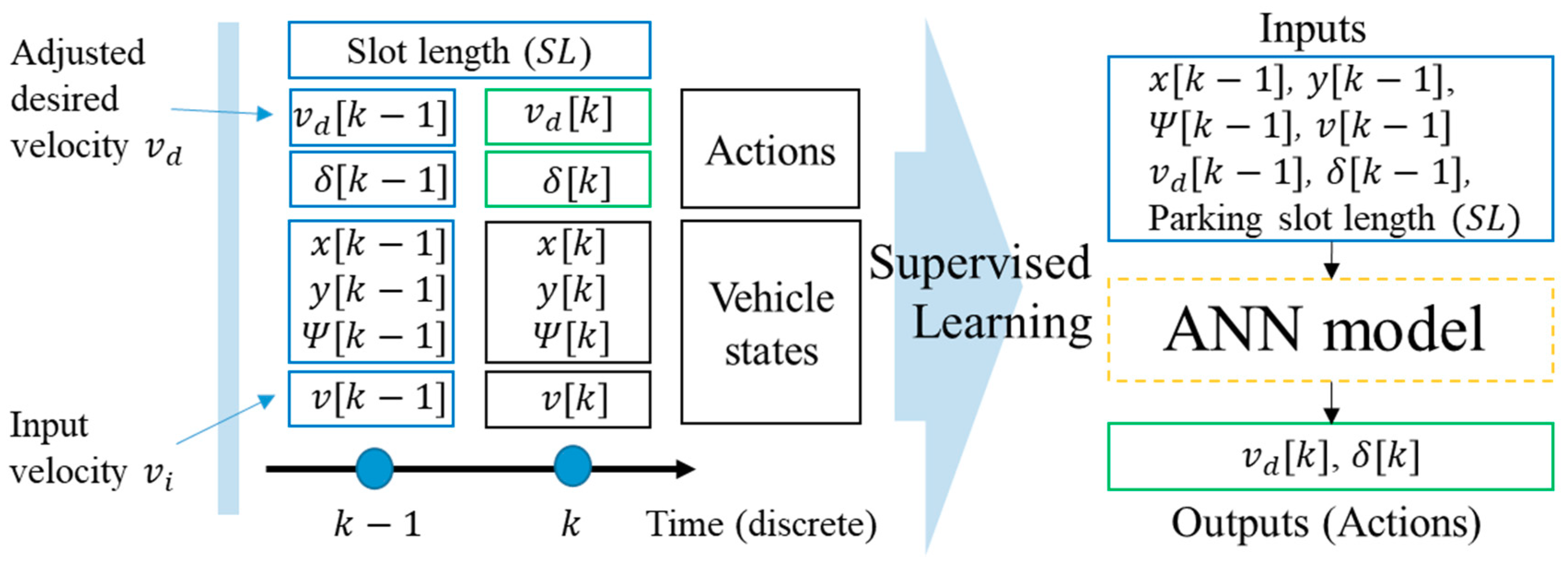
Modifying the automatic parking controller using an ANN [23], we constituted the automatic parking controller based on the proposed ANN model shown in Figure 7. The proposed ANN consisted of seven fully connected layers with 128 neurons in each layer and with seven inputs and two outputs. Hyperbolic tangent activation functions (tanh) were used in each fully connected layer. The inputs consist of the states of the vehicle at time k − 1 ($x\left[k-1\right]$, $y\left[k-1\right]$, $\Psi \left[k-1\right]$, and $v\left[k-1\right]$) and the parking slot length ($SL$) and actions of the vehicle at time k − 1 ($v_d\left[k-1\right]$ and $\delta \left[k-1\right]$). Then, actions of the vehicle at time k ($v_d\left[k\right]$ and $\delta \left[k\right]$) are outputs of the neural network for supervised learning. In the dataset, 103,650 inputs and outputs pairs sampled with a period of 0.1 s were included, where trajectories with single-maneuver include approximately 60–70 pairs of states, but multiple-maneuver trajectories include approximately 90–150 pairs of states.

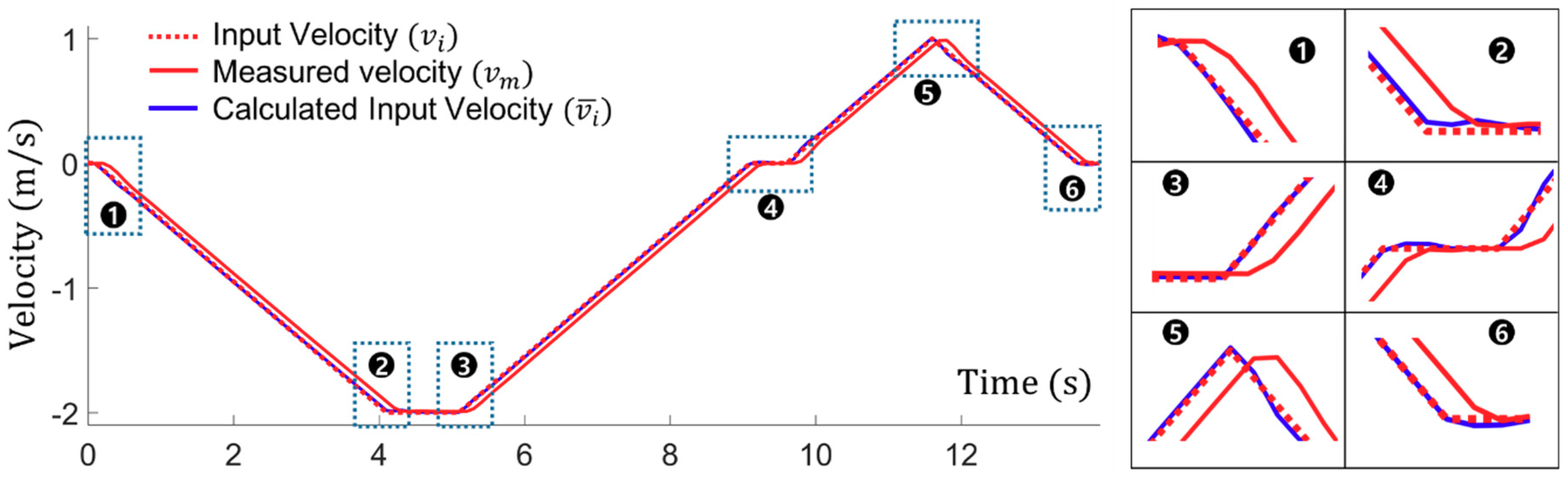
The trained ANN was the core of the automatic parking controller, which maneuvered the vehicle with parking skills learned from the training data, so as to produce the appropriate action outputs, while maneuvering the vehicle with respect to its current state and previous actions. The key idea of the proposed ANN was learning from the adjusted dataset using the inverse vehicle model to yield the adjusted desired velocity. Profiles of the adjusted desired velocity were calculated using the input velocity using the inverse vehicle model.

We trained the ANN by applying a supervised learning method using the dataset with a mean squared error (MSE) loss function. We divided the dataset into training and validation data in the ratio of 80% and 20%. The proposed deep neural network was implemented using the Caffe deep learning framework [30]. It was trained through 1000 epochs with a randomly sampled batch (size of 64). The learning rate was 0.001, with a descent ratio of 0.96 per 10,000 iterations.

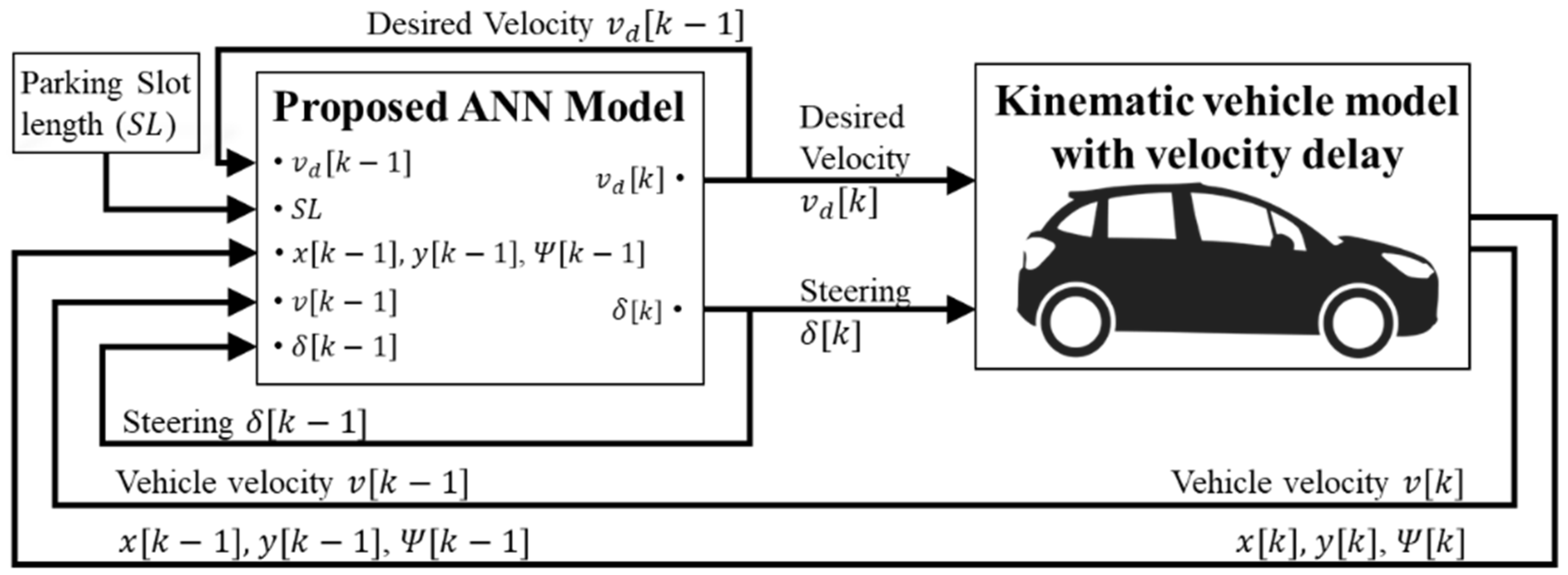
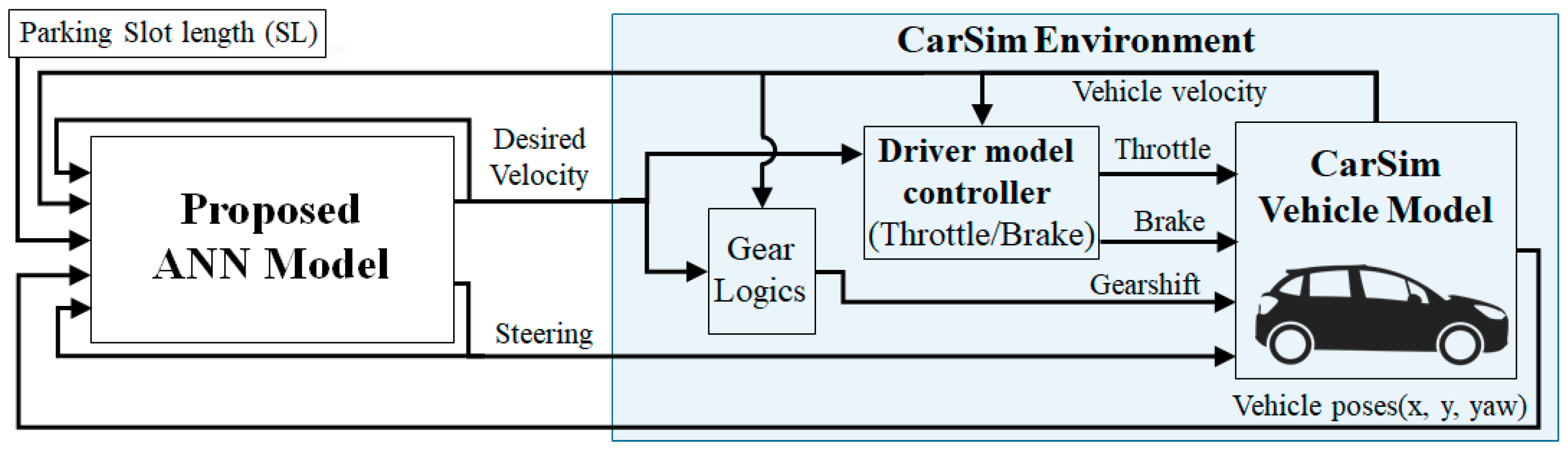
The proposed ANN parking controller and kinematic model of a vehicle constituted a software-in-the-loop (SIL) architecture for validation of the proposed approach, as illustrated in Figure 8. The SIL architecture has a feedback control loop, wherein the trained ANN generates action signals (desired velocity $v_d\left[k\right]$ and steering angle $\delta \left[k\right]$) as outputs and the vehicle poses ($x\left[k-1\right]$, $y\left[k-1\right]$, $\Psi \left[k-1\right]$), vehicle velocity $v\left[k-1\right]$, and previous action ($v_d\left[k-1\right]$ and $\delta \left[k-1\right]$) as inputs to be fed into the ANN at every time step, while running parking tasks. Compared with the conventional ANN model [23], the proposed ANN model had two terms of input velocity for the desired and vehicle velocity in order to consider the latency of longitudinal velocity.

4. Simulations and Discussions

The SIL architecture composed by the proposed ANN parking controller was simulated using MATLAB and CarSim vehicle simulator. Figure 8 shows the parking controller and kinematic vehicle model composing the (SIL) structure in MATLAB. We conducted MATLAB simulations for two cases: The first one was the parking controller trained with a dataset generated from an ideal vehicle without longitudinal latency and a kinematic vehicle model without a longitudinal response delay. For the second case, the parking controller was trained with a dataset that had adjusted longitudinal latency by applying the inverse vehicle model and a kinematic vehicle model with a second-order longitudinal response delay described in Section 2. Both simulation cases of automatic parking were conducted under the same environmental conditions. The parking task began at the ready-to-reverse point (RRP), where the vehicle started to move backwards toward the destination position in the parking slot. The parking process was complete when the vehicle reached the designated parking slot with the requirements for the final pose of automatic parking, as described by the ISO 16787 standard [31].

4.1. MATLAB Simulation Results

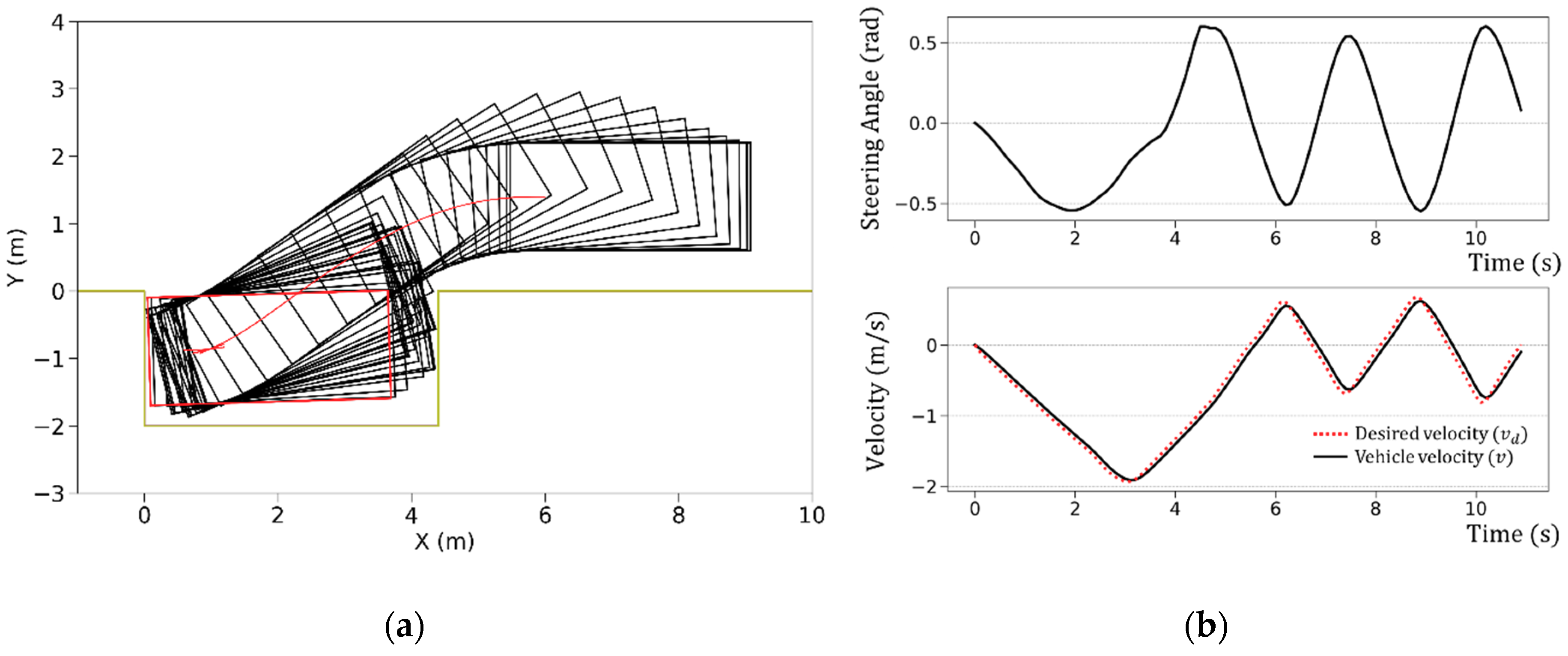
Figure 9 shows the results of the parking controller and ideal vehicle kinematic model without longitudinal delay based on the automatic parking controller using an ANN [23]. Figure 9a shows the results of consequential parking trajectories in the case of multiple maneuverings. Even with a small parking slot length (SL) (4.4 m) such that the vehicle had to change gears for back-and-forth movement, the conventional parking controller successfully completed parking in the tiny space with the ideal kinematic vehicle model.

Figure 10 shows the simulation results of the SIL structure composed of the kinematic vehicle model that has longitudinal velocity delay approximated with the values of the coefficients ${\alpha }_1$, ${\alpha }_0,$ and ${\beta }_0$ at 0.8284, –0.3267, and 0.4968, respectively.

The neural network learned to properly maneuver the vehicle even for back-and-forth movement to prevent a collision in the tiny space. The MATLAB simulation results demonstrate that the parking controller generated appropriate online maneuvers to complete the parking when the ANN model was trained with the dataset generated by the same vehicle model as the kinematic model in the SIL.

4.2. Simulation Results of the CarSim Vehicle Simulator

We simulated vehicle dynamics behavior with a realistic SIL configuration using the CarSim vehicle simulator. We composed a SIL structure for CarSim as shown in Figure 11. The dynamics model consisted of the following components: Engine, transmission, chassis, and gear-shift logic. A vehicle model having the same kinematic model coefficients (L/l_w = 3.6/2.53) utilized in the dataset generation [23] was used in this simulation. In addition to the kinematic model, we adopted a gearshift logic similar to a real vehicle to consider the time required to change gears when the moving direction changed for multiple maneuverings. The logic held a zero velocity for 0.8 s when the longitudinal velocity changed from positive to negative, or vice versa.

We conducted CarSim simulations for these two cases: In the first case, the ANN trained with the dataset generated from an ideal vehicle model without canceled latency, and in the second case, the ANN trained with the dataset adjusted by the proposed inverse vehicle model.

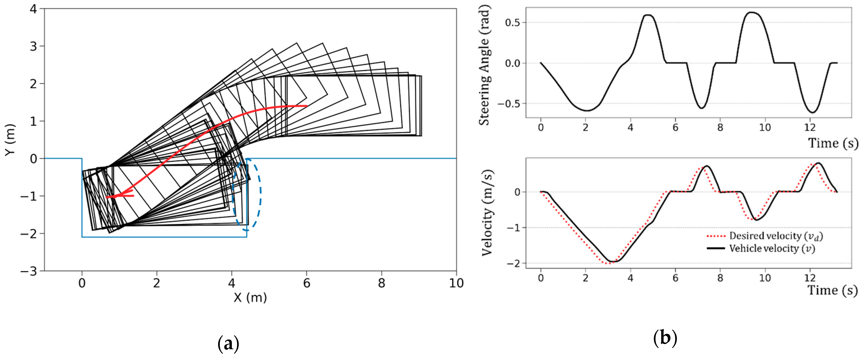
Figure 12 shows the simulated results of the first case when the conditions of SL = 4.4 m, and RRP was at the position $(x_{RRP}$, $y_{RRP}$) = (6.0, 1.4). The front right side of the vehicle can be seen to have collided with the borderline of the slot, whose area is indicated by blue dotted lines in Figure 12a. On the other hand, the simulated results of the second case with the same parking environmental conditions, the automatic parking was completed successfully without collision through multiple back-and-forth movements, as shown in Figure 13. The ANN parking controller trained with the dataset adjusted by the proposed inverse vehicle model learned to yield accurate automatic parking maneuvers without collision in a confined space.

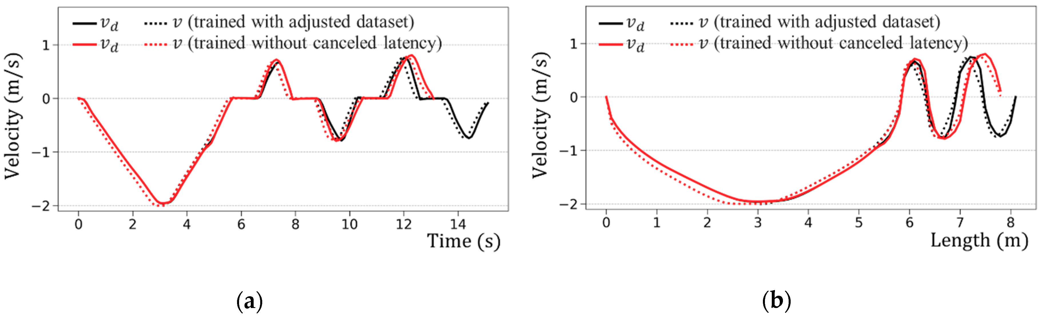
Figure 14 shows the simulated velocity input profiles of the driver model for the parking controller trained with the adjusted or un-adjusted dataset. At the beginning of the parking maneuver, no significant difference between two cases existed; however, the error became severe after two back-and-forth movements around a lap time of 12 s (or after moving distance was more than 7 m).

4.3. Discussions

We simulated automatic parking for different vehicle models (kinematic and CarSim vehicles) and parking controllers consisting of an ANN trained with a dataset with and without adjustment using the proposed inverse vehicle model, as listed in

Table 1. Success rates of automatic parking on test conditions.

Parking Controller	Ratio of Successful Parking
	MATLAB Simulations (Kinematics)	CarSim Simulations (Dynamics)
ANN trained with dataset without canceled latency	99.1% (with ideal vehicle model without latency)	41%
ANN trained with dataset adjusted by Proposed inverse vehicle model	98.9% (with vehicle model, including latency)	96%

. We defined an area of the initial starting points by the union of x- and y- coordinates’ boundaries for the generation of the training dataset. For the simulations, we chose random starting points in the union, which are not included in the training dataset. We conducted 1000 MATLAB simulations and 100 CarSim simulations. We defined the fail-condition if the main vehicle failed to reach the destination, satisfying the requirement defined in ISO 16787 [31] of within 30 s. Table 1 shows a summary of the simulated success ratios of the automatic parking, with simple kinematic and dynamic models close to the realistic vehicle simulations. The success ratio of the ANN trained with dataset without canceled latency was up to 99% in the MATLAB simulation when the kinematic model of the ideal vehicle model was used. However, in the CarSim simulation, the ratio dropped to 41%. The parking controller trained with the adjusted dataset using the inverse vehicle model showed that the success rate dropped less than 3% in the CarSim dynamic simulations.

Conventional controllers without canceled latency effects can successfully perform parking maneuvers when both the vehicle model generating the dataset for training the ANN and the kinematic vehicle model are almost equal and nearly ideal without the longitudinal latency. The generalization capability of the network is mostly determined by system complexity and training of the network. Poor generalization may be observed when the network is over-fitted or system complexity is relatively more than the training data. To reach the generalization, the dataset should be split into three parts: the training dataset, the validation dataset, and a test dataset. We carried out the training, validation, and testing steps during the development of the proposed ANN-based automatic parking controller. We divided the dataset into training and validation data in the ratio of 80% and 20%. In addition to the dataset split method, we conducted simulations with additional consideration to improve the generalization capability of the proposed ANN-based parking controller. The training dataset was generated by using a bicycle kinematic model. However, we simulated the parking controller using a CarSim simulator with dynamic models that are different from the kinematic model used in the dataset generation. We obtained a success rate of 96%, when the proposed Inverse vehicle model was applied to cancel the longitudinal latency. The success rate without applying the inverse vehicle model was only 41%. We also considered variation in the vehicle’s overall length in the ANN-based automatic parking controller in our previous research [23]. Our results in previous work showed that the ANN-based parking controller (with twin architecture) can successfully perform parking maneuvers without retraining while the variations in the vehicle’s overall length are less than 5% [23].

The parking controller, consisting of an ANN trained with a dataset adjusted by the inverse vehicle model, prevents the mismatch in the temporal synchronization between lateral and longitudinal control signals by compensating the effect of the vehicle’s longitudinal latency. The simulation results with the various vehicle models provide substantial evidence that the proposed inverse vehicle model trained ANN model learned more robust parking skills compared with the conventional methods.

However, in this study, we did not consider the changes of environmental factors, such as surface conditions of the road, weight, and distribution of the mounted load, aging of vehicles, inclined parking lots, etc., that may cause uncertainty in the trajectory of the vehicle during automatic parking maneuvers. As a further work we need an experimental validation of the proposed automatic parking controller, including changes in environmental factors for the real-world applications.

5. Conclusions

We proposed an integrated longitudinal and lateral controller for automatic parking by training an ANN on a dataset using an inverse vehicle model. The inverse vehicle model calculates the adjusted desired velocity with which the vehicle can output the previously planned velocity. By learning the current vehicle states and the corresponding actions applied with the inverse vehicle model, the proposed automatic parking controller can yield a direct steering angle and desired velocity online, predicting the relationships of the desired and vehicle velocities. The proposed trained ANN model can compensate a vehicle’s longitudinal latency and mismatches, while the controller maneuvers the vehicle according to a planned desired velocity and steering profiles. Using a vehicle dynamics model, we validated that the ANN controller trained with the adjusted dataset by the proposed inverse vehicle model can complete automatic parking, even with multiple back-and-forth movements in a confined space.

References

1. Suhr, J.; Jung, H.; Suhr, J.K.; Jung, H.G. A universal vacant parking slot recognition system using sensors mounted on off-the-shelf vehicles. Sensors 2018, 18, 1213. [Google Scholar] [CrossRef] [PubMed]
2. Amiri, W.A.; Baza, M.; Banawan, K.; Mahmoud, M.; Alasmary, W.; Akkaya, K. Privacy-preserving smart parking system using blockchain and private information retrieval. arXiv 2019, arXiv:1904.09703. [Google Scholar]
3. Gómez-Bravo, F.; Cuesta, F.; Ollero, A.; Viguria, A. Continuous curvature path generation based on β-spline curves for parking manoeuvres. Robot. Auton. Syst. 2008, 56, 360–372. [Google Scholar] [CrossRef]
4. Moon, J.; Bae, I.; Cha, J.G.; Kim, S. A trajectory planning method based on forward path generation and backward tracking algorithm for Automatic Parking Systems. In Proceedings of the 17th International IEEE Conference on Intelligent Transportation Systems (ITSC), Qingdao, China, 8–11 October 2014. [Google Scholar]
5. Bae, I.; Kim, J.H.; Moon, J.; Kim, S. Lane Change Maneuver based on Bezier Curve providing Comfort Experience for Autonomous Vehicle Users. In Proceedings of the 2019 IEEE 22th International Conference on Intelligent Transportation Systems (ITSC); IEEE, Auckland, New Zealand, 27–30 October 2019; p. 6. [Google Scholar]
6. Vorobieva, H.; Glaser, S.; Minoiu-Enache, N.; Mammar, S. Automatic parallel parking in tiny spots: Path planning and control. IEEE Trans. Intell. Transp. Syst. 2015, 16, 396–410. [Google Scholar] [CrossRef]
7. Du, X.; Tan, K.K. Autonomous reverse parking system based on robust path generation and improved sliding mode control. IEEE Trans. Intell. Transp. Syst. 2015, 16, 1225–1237. [Google Scholar] [CrossRef]
8. Bae, I.; Kim, J.H.; Kim, S. Adaptive preview control of single-point path tracker for car-like delivery service robot. Electron. Lett. 2019. [Google Scholar] [CrossRef]
9. Zips, P.; Böck, M.; Kugi, A. Optimisation based path planning for car parking in narrow environments. Robot. Auton. Syst. 2015, 79, 1–11. [Google Scholar] [CrossRef]
10. Li, B.; Shao, Z. Simultaneous dynamic optimization: A trajectory planning method for nonholonomic car-like robots. Adv. Eng. Softw. 2015, 87, 30–42. [Google Scholar] [CrossRef]
11. Li, B.; Shao, Z. A unified motion planning method for parking an autonomous vehicle in the presence of irregularly placed obstacles. Knowl. Based Syst. 2015, 86, 11–20. [Google Scholar] [CrossRef]
12. Li, B.; Wang, K.; Shao, Z. Time-optimal maneuver planning in automatic parallel parking using a simultaneous dynamic optimization approach. IEEE Trans. Intell. Transp. Syst. 2016, 17, 3263–3274. [Google Scholar] [CrossRef]
13. Moon, J.; Bae, I.; Kim, S. Real-Time near-optimal path and maneuver planning in automatic parking using a simultaneous dynamic optimization approach. In Proceedings of the IEEE Intelligent Vehicles Symposium, Los Angeles, CA, USA, 11–14 June 2017; pp. 193–196. [Google Scholar]
14. Michalek, M.M. Modular approach to compact low-speed kinematic modelling of multi-articulated urban buses for motion algorithmization purposes. In Proceedings of the Institute of Electrical and Electronics Engineers (IEEE), Paris, France, 9–12 June 2019; pp. 2060–2065. [Google Scholar]
15. Gawron, T.; Michalek, M.M. A G3-continuous extend procedure for path planning of mobile robots with limited motion curvature and state constraints. Appl. Sci. 2018, 8, 2127. [Google Scholar] [CrossRef]
16. Li, B.; Shao, Z. An incremental strategy for tractor-trailer vehicle global trajectory optimization in the presence of obstacles. In Proceedings of the 2015 IEEE International Conference on Robotics and Biomimetics, Zhuhai, China, 6–9 December 2015; pp. 1447–1452. [Google Scholar]
17. Lee, J.Y.; Kim, M.S.; Lee, J.J. Design of fuzzy controller for car parking problem using evolutionary multi-objective optimization approach. In Proceedings of the IEEE International Symposium on Industrial Electronics, Montreal, QC, Canada, 9–13 July 2006; Volume 1, pp. 329–334. [Google Scholar]
18. Yin Aye, Y. Design of an Image-based Fuzzy Controller for Parking Problems of a Car-like Mobile Robot. Ph.D. Thesis, Okayama University, Okayama, Japan, 2017. [Google Scholar]
19. Zhao, Y.; Collins, E.G. Robust automatic parallel parking in tight spaces via fuzzy logic. Robot. Auton. Syst. 2005, 51, 111–127. [Google Scholar] [CrossRef]
20. Liu, W.; Li, Z.; Li, L.; Wang, F.Y. Parking like a human: A direct trajectory planning solution. IEEE Trans. Intell. Transp. Syst. 2017, 18, 3388–3397. [Google Scholar] [CrossRef]
21. Li, R.; Wang, W.; Chen, Y.; Srinivasan, S.; Krovi, V.N. An end-to-end fully automatic bay parking approach for autonomous vehicles. In Proceedings of the ASME 2018 Dynamic Systems and Control Conference (DSCC 2018), Atlanta, GA, USA, 30 September–3 October 2018; Volume 2, p. 8. [Google Scholar]
22. Rathour, S.; John, V.; Nithilan, M.K.; Mita, S. Vision and dead reckoning-based end-to-end parking for autonomous vehicles. In Proceedings of the IEEE Intelligent Vehicles Symposium, Changshu, China, 26–30 June 2018; pp. 2182–2187. [Google Scholar]
23. Moon, J.; Bae, I.; Kim, S. Automatic parking controller with a twin artificial neural network architecture. Math. Probl. Eng. 2019, 2019, 1–18. [Google Scholar] [CrossRef]
24. Nie, L.; Guan, J.; Lu, C.; Zheng, H.; Yin, Z. Longitudinal speed control of autonomous vehicle based on a self-adaptive PID of radial basis function neural network. IET Intell. Transp. Syst. 2018, 12, 485–494. [Google Scholar] [CrossRef]
25. Chen, L.; Li, J.; Ding, R. Identification for the second-order systems based on the step response. Math. Comput. Model. 2011, 53, 1074–1083. [Google Scholar] [CrossRef]
26. Yang, D.; Ding, R. Transforms from differential equations to difference equations and vice-versa applied to computer control systems. Appl. Math. Lett. 2014, 31, 18–24. [Google Scholar] [CrossRef]
27. Mechanical Simulation Corporation, CarSim Reference Manual. Available online: https://carsim.com (accessed on 20 October 2019).
28. Biegler, L.T. An overview of simultaneous strategies for dynamic optimization. Chem. Eng. Process. Process Intensif. 2007, 46, 1043–1053. [Google Scholar] [CrossRef]
29. Biegler, L.T. Nonlinear Programming: Concepts, Algorithms and Applications to Chemical Processes; Siam: Philadelphia, PA, USA, 2010; Volume 40, ISBN 978-0-898717-02-0. [Google Scholar]
30. Jia, Y.; Shelhamer, E.; Donahue, J.; Karayev, S.; Long, J.; Girshick, R.; Guadarrama, S.; Darrell, T. Caffe: Convolutional Architecture for Fast Feature Embedding. In Proceedings of the 22nd ACM International Conference on Multimedia, Orlando, FL, USA, 3–7 November 2014. [Google Scholar]
31. ISO 16787:2017 Intelligent Transport Systems—Assisted Parking System (APS)—Performance Requirements and Test Procedures. Available online: https://www.iso.org/standard/73768.html (accessed on 5 May 2019).
32. Attia, R.; Orjuela, R.; Basset, M. Combined longitudinal and lateral control for automated vehicle guidance. Veh. Syst. Dyn. 2014, 52, 261–279. [Google Scholar] [CrossRef] [Green Version]
33. Rajamani, R. Vehicle Dynamics and Control; Mechanical Engineering Series; Springer: Boston, MA, USA, 2012; ISBN 978-1-4614-1432-2. [Google Scholar]
34. Boulkroune, B.; Van Aalst, S.; Lehaen, K.; De Smet, J. Observer-based controller with integral action for longitudinal vehicle speed control. In Proceedings of the IEEE Intelligent Vehicles Symposium, Los Angeles, CA, USA, 11–14 June 2017; pp. 322–327. [Google Scholar]
Figure 1. Typical block diagram of a conventional automatic parking control system.
Electronics 08 01452 g001
Figure 2. Example of automatic parking when a trajectory is planned without regard to the latency of the longitudinal response: (a) The planned and simulated trajectories without accounting for longitudinal latency; (b) the planned and simulated steering angles and velocity profiles. Longitudinal latency causes a mismatch in time synchronization between the velocity and steering control signals.
Electronics 08 01452 g002
Figure 3. The proposed steps for developing the inverse vehicle model for the neural network-based parking controller. Here, v m is the measured vehicle velocity in association with the input v i , v d is the adjusted desired velocity, and v is the vehicle velocity when v d is applied to the driver model.
Electronics 08 01452 g003
Figure 4. Input velocity profile and corresponding CarSim simulated vehicle velocity, and the calculated input velocity using Equation (3).
Electronics 08 01452 g004
Figure 5. A simulated example of adjusted desired velocity ( v d ) , vehicle velocity ( v m d ) driven by v d .
Electronics 08 01452 g005
Figure 6. The simulated results of (a) parking trajectory with and without cancelation of the longitudinal latency, and (b) profiles of the steering angle control signal along with input velocity ( v i ) , adjusted desired velocity ( v d ) , and vehicle velocity driven by v d ( v m d ).
Electronics 08 01452 g006
Figure 7. Structure of the artificial neural network (ANN) model of the parking controller and arrangement of input and output data in the training dataset.
Electronics 08 01452 g007
Figure 8. Automatic parking controller based on the proposed ANN model.
Electronics 08 01452 g008
Figure 9. The simulated results of the parking controller with the ANN model containing the ideal vehicle model without longitudinal delay: (a) the simulated parking trajectory and.(b) profiles of the steering angle and velocity, in the case of SL = 4.4 and ready-to-reverse point (RRP) at position ( x R R P , y R R P ) = (6.0, 1.4).
Electronics 08 01452 g009
Figure 10. The simulated results of the proposed parking controller with kinematic vehicle model, including longitudinal delay: (a) The simulated parking trajectory and (b) profiles of the steering angle, desired velocity, and vehicle velocity in a case of SL = 4.4 and RRP at position ( x R R P , y R R P ) = (6.0, 1.4).
Electronics 08 01452 g010
Figure 11. Structure of software-in-the-loop for the CarSim vehicle simulator.
Electronics 08 01452 g011
Figure 12. The simulated results using CarSim simulator with ANN controller trained with dataset having longitudinal latency without latency canceling procedure when SL = 4.4 and RRP at position ( x R R P , y R R P ) = (6.0, 1.4). (a) Simulated parking trajectory and (b) profiles of steering angle, desired velocity, and vehicle velocity.
Electronics 08 01452 g012
Figure 13. The simulated results using CarSim with the proposed ANN controller trained with the dataset adjusted by the proposed inverse vehicle model when SL = 4.4 and RRP at position ( x R R P , y R R P ) = (6.0, 1.4): (a) Simulated parking trajectory and (b) profiles of the steering angle, desired velocity, and vehicle velocity.
Electronics 08 01452 g013
Figure 14. The simulated results of the velocity profile of parking under the environment condition of SL = 4.4 and RRP at position ( x R R P , y R R P ) = (6.0, 1.4). (a) x-axis with time and (b) x-axis with respect to the length of moving distance.
Electronics 08 01452 g014