New “Full-Bridge Buck Inverter–DC Motor” System: Steady-State and Dynamic Analysis and Experimental Validation

Abstract

A mathematical model of a new “full-bridge Buck inverter–DC motor” system is developed and experimentally validated. First, using circuit theory and the mathematical model of a DC motor, the dynamic behavior of the system under study is deduced. Later, the steady-state, stability, controllability, and flatness properties of the deduced model are described. The flatness property, associated with the mathematical model, is then exploited so that all system variables and the input can be differentially parameterized in terms of the flat output, which is determined by the angular velocity. Then, when a desired trajectory is proposed for the flat output, the input signal is calculated offline and is introduced into the system. In consequence, the validation of the mathematical model for constant and time-varying duty cycles is possible. Such a validation of this mathematical model is tackled from two directions: (1) by circuit simulation through the SimPowerSystems toolbox of Matlab-Simulink and (2) via a prototype of the system built by using Matlab-Simulink and a DS1104 board. The good similarities between the circuit simulation and the experimental results allow satisfactorily validating the mathematical model.

1. Introduction

Electronic power converters as drivers for DC motors have been recently studied [1,2,3,4,5,6,7,8,9,10,11,12,13,14,15,16,17,18,19,20,21,22,23,24,25,26,27,28,29,30]. According to the literature on power converters, the Buck [1,2,3,4,5,6,7,8,9,10,11,12,13,14,15,16,17,18,19,20,21,22,23], the Boost [24,25,26], and the Buck-Boost [27,28,29,30] topologies are the most used. The Buck topology received the most attention. This is, in part, due to the fact that the mathematical model of the Buck topology is linear and, compared with the Boost and the Buck-Boost topologies, the Buck topology does not have a nonminimum phase output variable [31]. As the present paper focuses on the Buck power converter as a driver for a DC motor, a review of state-of-the-art of this topic is presented below.

1.1. Related Work

The literature reviewed has been divided into two approaches: (1) DC/DC Buck converter–DC motor systems [1,2,3,4,5,6,7,8,9,10,11,12,13,14,15,16,17,18,19,20] and (2) DC/DC Buck converter–inverter–DC motor systems [21,22,23].

Regarding a DC motor when it is fed by a DC/DC Buck converter, the most relevant literature is the following; Lyshevski, in [1], designed a nonlinear PI control that regulates the velocity of the motor shaft. Ahmad et al., in [2], presented a performance assessment of the PI, fuzzy PI, and LQR controls for the tracking problem. Bingöl and Paçaci reported, in [3], a virtual laboratory based on neural networks to control the angular velocity. Sira-Ramírez and Oliver-Salazar [4] used the concepts of active disturbance rejection and differential flatness to design a tracking control for two configurations of a DC/DC Buck converter connected to a DC motor. In [5], Silva-Ortigoza et al. introduced a two-stage sensorless tracking control based on flatness, whose implementation was executed via a $\mathsf{\Sigma }$–$\Delta$-modulator. In [6], Hoyos et al. designed a robust adaptive quasi-sliding mode regulation control, which is generated through the zero average dynamics (ZAD) technique and a fixed point inducting control (FPIC). Later, Silva-Ortigoza et al. proposed a robust hierarchical control approach based on differential flatness in [7]. Wei et al. in [8] reported a robust adaptive controller based on dynamic surface and sliding mode. A two-stage controller based on sliding mode plus PI control and flatness was reported by Silva-Ortigoza et al. in [9]. Hernández-Guzmán et al., in [10], proposed a simple control scheme by using sliding mode, to regulate the converter current, and three PI controls. These latter to regulate the converter voltage, the motor current, and the angular velocity. Moreover, via sensorless load torque estimation schemes, a passive tracking control based on the exact tracking error dynamics was proposed by Kumar and Thilagar in [11]. Khubalkar et al., in [12], presented the design and realization of standalone digital fractional order PID control for the Buck converter–DC motor system, where the dynamic particle swarm optimization (dPSO) technique is used to tune the gains and the order of the control. By using the concept of differential flatness and a derivative-free nonlinear Kalman filter, Rigatos et al., in [13], designed a control to solve the trajectory tracking problem. Another solution was proposed by Nizami et al. in [14], where a neuroadaptive backstepping tracking control was developed for the system. The dynamic analysis of the Buck converter that uses the combined ZAD-FPIC technique to control the speed of the DC motor, when different reference values are considered, was developed in [15] by Hoyos et al. Khubalkar et al., in [16], presented for the DC/DC Buck converter driving a DC motor a digital implementation of a fractional order PID control, whose parameters are tuned through the improved inertia weight dPSO technique. A flatness-based tracking control implemented in successive loops was presented by Rigatos et al. in [17]. More recently, the speed regulation problem was addressed by Yang et al. in [18], by using a robust predictive control via a discrete-time reduced-order GPI observer. Additionally, other important contributions related to the connection of a DC/DC Buck converter and a DC motor have been reported in [19,20].

On the other hand, regarding a DC motor when it is fed by a DC/DC Buck converter–inverter, the literature is as follows. In [21], Silva-Ortigoza et al. developed and experimentally validated a mathematical model associated with the DC/DC Buck converter–inverter–DC motor system. Silva-Ortigoza et al. reported, in [22], a passive tracking control based on the exact tracking error dynamics. Robust tracking controls were proposed by Hernández-Márquez et al. in [23].

1.2. Discussion of Related Work and Contribution

In accordance with the aforementioned, different approaches have been proposed for a DC motor fed by a DC/DC Buck converter when the unidirectional rotation of the motor shaft is considered [1,2,3,4,5,6,7,8,9,10,11,12,13,14,15,16,17,18,19]. This unidirectional rotation emerges because the Buck converter only delivers unipolar voltages. In this regard, when an inverter is integrated between the converter and the DC motor, bidirectional rotation of the motor shaft is achieved, giving rise to the “DC/DC Buck converter–inverter–DC motor” system [21]. Related to this system, the trajectory tracking problem has been addressed in [22,23]. Note that as such a system includes an inverter connected to the DC motor, an abrupt behavior of the voltages and currents is generated because of the hard switching of the transistors composing the inverter; consequently, the useful life of the DC motor could be reduced. One manner to attenuate the abruptness of the voltages and currents and at the same time to drive a bipolar voltage to the DC motor is through the full-bridge Buck inverter, giving rise to the new “full-bridge Buck inverter–DC motor” system [32]. Thus, compared with [32], the contribution of the present paper is fourfold:

• The steady-state, stability, controllability, and flatness properties associated with the dynamic behavior of the “full-bridge Buck inverter–DC motor” system are presented.
• The differential flatness property [33] linked to the mathematical model of the system under study is exploited, with the aim of obtaining the reference trajectories of the system offline so that the mathematical model can be validated when time-varying duty cycles are considered.
• Obtaining circuit simulation results when the input and the reference signals are introduced into the system via the SimPowerSystems toolbox of Matlab-Simulink.
• Obtaining experimental results when the input and the reference signals are introduced to a prototype of the system built through Matlab-Simulink along with a DS1104 board.

The remainder of this paper is organized as follows. In Section 2, the generalities of the full-bridge inverter DC–motor system and some static/dynamic properties and the generation of the reference trajectories, via the flatness concept, are presented. To validate the proposed mathematical model, in Section 3, circuit simulation and experimental results are shown. Later, a discussion of the obtained results is introduced in Section 4. Finally, concluding remarks are given in Section 5.

2. Materials and Methods

This section describes the key concepts of the full-bridge Buck inverter–DC motor system. First, the mathematical model of the system is obtained by using the circuit theory and the mathematical model of a DC motor. Second, some static and dynamic properties related to the deduced model are listed. Last, the generation of the reference trajectories is introduced.

2.1. Model of the “Full-Bridge Buck Inverter–DC Motor” System

In the following, the generalities of the full-bridge Buck inverter–DC motor system and the deduction of its corresponding mathematical model are presented.

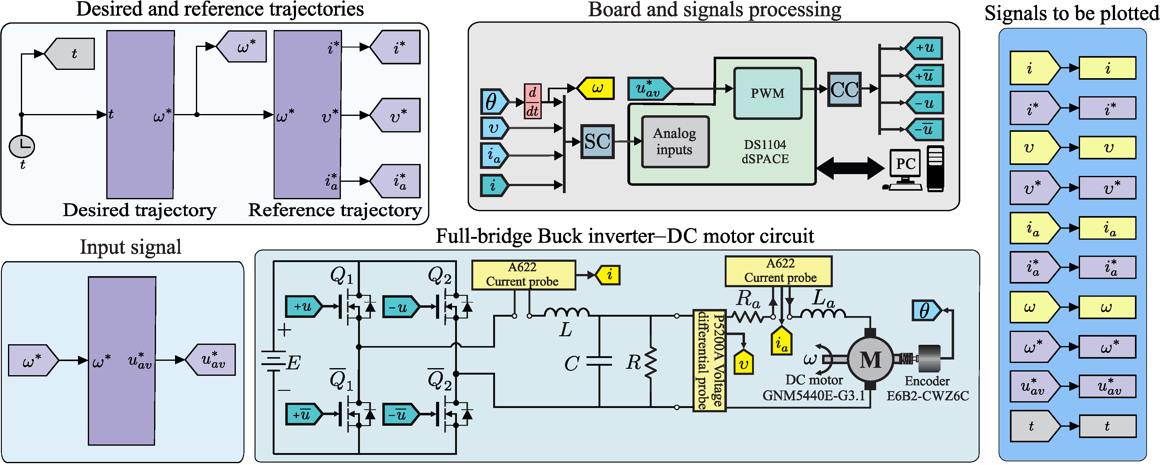
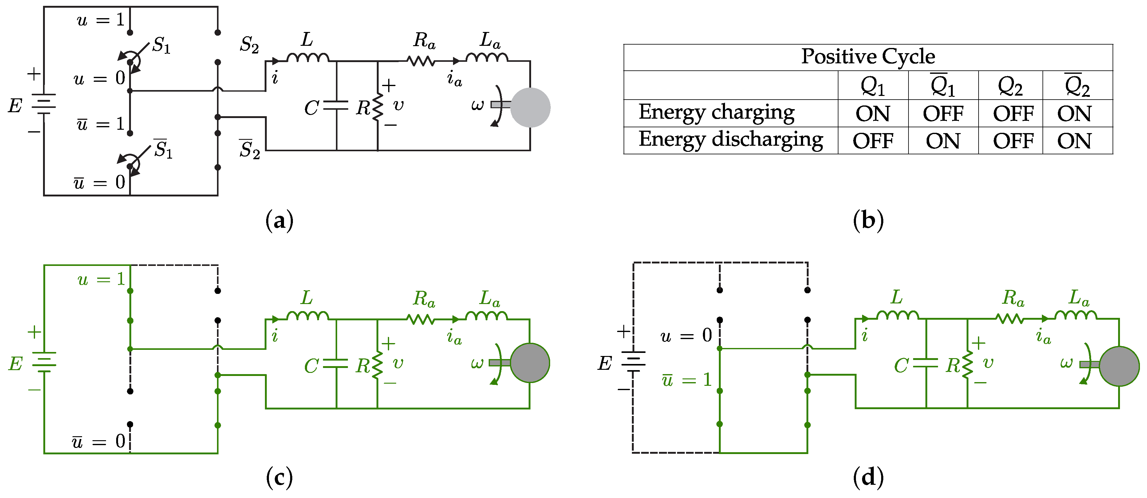
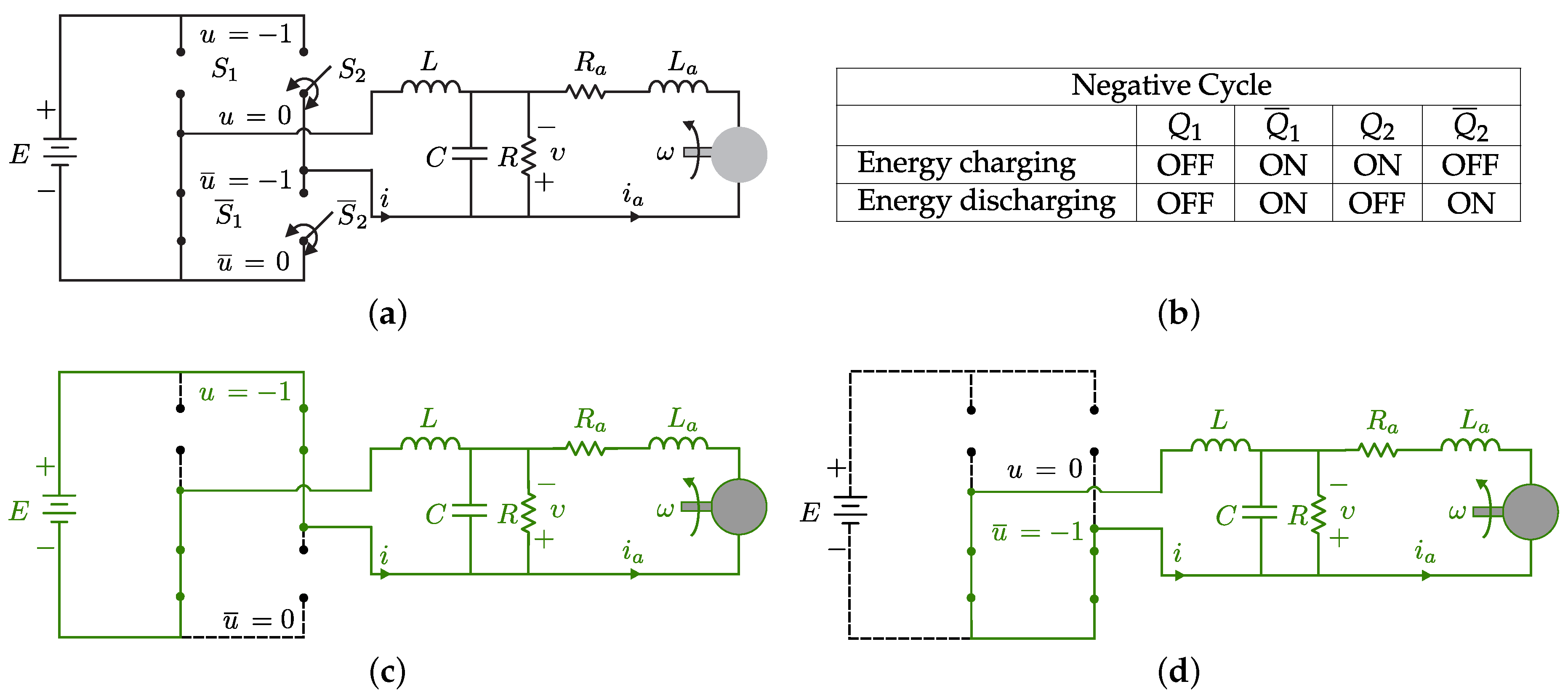
2.1.1. Generalities of the Full-Bridge Buck Inverter–DC Motor System

The electronic diagram of the full-bridge Buck inverter–DC motor topology is drawn in Figure 1a. Such a circuit can be divided into two parts: (1) the full-bridge Buck inverter and (2) the DC motor. The full-bridge Buck inverter modulates and supplies the bipolar voltage $\upsilon$ to the DC motor via the input signal u. This part also contains the following; a power supply E; an array of four MOSFET transistors—$Q_1$, ${\overline{Q}}_1$, $Q_2$, and ${\overline{Q}}_2$; and a low-pass filter composed of R, C, and L (where the current i flows through). In addition, the DC motor is the actuator of the system and is made up of the elements $L_a$, $R_a$ and a variable $i_a$, corresponding to the inductance, resistance, and armature current. Here, $\omega$ is the angular velocity of the shaft. Other important values of the DC motor are b, $k_m$, J, and $k_e$, which correspond to the viscous friction coefficient of the motor, the motor torque constant, the moment of inertia of the rotor, and the counterelectromotive force constant, respectively. Additionally, Figure 1b depicts the ideal configuration of the system, which will be described in the following section.

2.1.2. Mathematical Model of the Proposed “Full-Bridge Buck Inverter–DC Motor” Topology

In Figure 1b, the ideal structure of the proposed “full-bridge Buck inverter–DC motor” topology is depicted. In this figure, the transistors $Q_1$, $Q_2$, ${\overline{Q}}_1$, and ${\overline{Q}}_2$ are replaced by switches $S_1$, $S_2$, ${\overline{S}}_1$, and ${\overline{S}}_2$, respectively. When switches $S_1$ or $S_2$ are on, the possible values of the input signal u are 1 or $-1$. These values depend on the voltage polarity, or operating cycle, that is desired to be generated in load R. That is, for a positive voltage, or positive cycle, the switch $S_1$ will be on and the input signal u will be 1. For a negative voltage, or negative cycle, the switch $S_2$ will be on and the output signal u will be $-1$. On the other hand, when switches $S_1$ and $S_2$ are off, the input signal u is 0. During this commutation process, the switches ${\overline{S}}_1$ and ${\overline{S}}_2$ are activated complementarily to $S_1$ and $S_2$. With the aim of easing the deduction of the mathematical model of the full-bridge Buck inverter–DC motor topology, different structures (associated with the positions of the inverter switches) will be analyzed. Thus, in accordance with the bipolarity of the voltage $\upsilon$, the deduction of the mathematical model will be divided into positive and negative cycles.

• Positive Cycle

The generation of a positive voltage, i.e., the clockwise movement of the motor shaft, is executed when the ideal circuit of Figure 1b is simplified to the circuit shown in Figure 2a. It is noteworthy that switches $S_2$ and ${\overline{S}}_2$ are in a fixed position, whereas switches $S_1$ and ${\overline{S}}_1$ work complementarily, switching their position according to the input signal u. Thus, similar to a Buck converter, the energy charging in the $LC$ filter occurs when the input signal $u=1$, whereas energy discharging occurs when $u=0$. This behavior is summarized in Figure 2b.

(i) Energy charging. In this mode of operation, a part of the energy supplied by the power supply is stored in the $LC$ filter. Figure 2c depicts the structure of this operating mode. By using the mathematical model of a DC motor [34,35] and applying Kirchhoff’s laws to the electric circuit of Figure 2c, the following system of differential equations is obtained:

$$\begin{array}{cc}\hfill L\frac{di}{dt}& =-\upsilon +E,\hfill \end{array}$$

(1)

$$\begin{array}{cc}\hfill C\frac{d\upsilon }{dt}& =i-\frac{\upsilon }{R}-i_a,\hfill \end{array}$$

(2)

$$\begin{array}{cc}\hfill L_a\frac{d{i}_a}{dt}& =\upsilon -R_a{i}_a-k_e\omega ,\hfill \end{array}$$

(3)

$$\begin{array}{cc}\hfill J\frac{d\omega }{dt}& =k_m{i}_a-b\omega .\hfill \end{array}$$

(4)

(ii) Energy discharging. Here, as the $LC$ filter is no longer connected to the power supply, the energy stored in the filter is released directly to the resistance R and to the DC motor. Figure 2d shows the connection of this operating mode. By using the mathematical model of a DC motor and applying Kirchhoff’s laws, the following system associated with the circuit of Figure 2d is obtained:

$$\begin{array}{cc}\hfill L\frac{di}{dt}& =-\upsilon ,\hfill \end{array}$$

(5)

$$\begin{array}{cc}\hfill C\frac{d\upsilon }{dt}& =i-\frac{\upsilon }{R}-i_a,\hfill \end{array}$$

(6)

$$\begin{array}{cc}\hfill L_a\frac{d{i}_a}{dt}& =\upsilon -R_a{i}_a-k_e\omega ,\hfill \end{array}$$

(7)

$$\begin{array}{cc}\hfill J\frac{d\omega }{dt}& =k_m{i}_a-b\omega .\hfill \end{array}$$

(8)

• Negative Cycle

In generating the negative voltage, the ideal circuit of Figure 1b reduces to the one shown in Figure 3a. Here, switches $S_1$ and ${\overline{S}}_1$ are in a fixed position, whereas switches $S_2$ and ${\overline{S}}_2$ work complementarily, switching their position according to the input u. Similarly to the positive cycle, there is energy charging or discharging in the $LC$ filter. This behavior is summarized in Figure 3b.

(i) Energy charging. The circuit allowing energy charging for negative cycles is shown in Figure 3c. The model related to the circuit of Figure 3c, after applying Kirchhoff’s laws and considering the mathematical model of a DC motor, is given by

$$\begin{array}{cc}\hfill L\frac{di}{dt}& =-\upsilon -E,\hfill \end{array}$$

(9)

$$\begin{array}{cc}\hfill C\frac{d\upsilon }{dt}& =i-\frac{\upsilon }{R}-i_a,\hfill \end{array}$$

(10)

$$\begin{array}{cc}\hfill L_a\frac{d{i}_a}{dt}& =\upsilon -R_a{i}_a-k_e\omega ,\hfill \end{array}$$

(11)

$$\begin{array}{cc}\hfill J\frac{d\omega }{dt}& =k_m{i}_a-b\omega .\hfill \end{array}$$

(12)

(ii) Energy discharging. Lastly, the energy discharging in this mode of operation is presented in Figure 3d. For this mode (see Figure 3d), the mathematical model is determined by the following system of differential equations:

$$\begin{array}{cc}\hfill L\frac{di}{dt}& =-\upsilon ,\hfill \end{array}$$

(13)

$$\begin{array}{cc}\hfill C\frac{d\upsilon }{dt}& =i-\frac{\upsilon }{R}-i_a,\hfill \end{array}$$

(14)

$$\begin{array}{cc}\hfill L_a\frac{d{i}_a}{dt}& =\upsilon -R_a{i}_a-k_e\omega ,\hfill \end{array}$$

(15)

$$\begin{array}{cc}\hfill J\frac{d\omega }{dt}& =k_m{i}_a-b\omega .\hfill \end{array}$$

(16)

By unifying the four modes (see Figure 2c,d, and Figure 3c,d), represented by Equations (1)–(16), the model of the full-bridge Buck inverter–DC motor topology is given by

$$\begin{array}{cc}\hfill L\frac{di}{dt}& =-\upsilon +Eu,\hfill \end{array}$$

(17)

$$\begin{array}{cc}\hfill C\frac{d\upsilon }{dt}& =i-\frac{\upsilon }{R}-i_a,\hfill \end{array}$$

(18)

$$\begin{array}{cc}\hfill L_a\frac{d{i}_a}{dt}& =\upsilon -R_a{i}_a-k_e\omega ,\hfill \end{array}$$

(19)

$$\begin{array}{cc}\hfill J\frac{d\omega }{dt}& =k_m{i}_a-b\omega ,\hfill \end{array}$$

(20)

where $u\in \{-1,0,1\}$ are the positions of the switches. Due to the discrete nature of the system modeled by Equations (17)–(20), it is usual to call it a “switched model”. In contrast, the continuous model or “average model” associated with the full-bridge Buck inverter–DC motor system is described by

$$\begin{array}{cc}\hfill L\frac{di}{dt}& =-\upsilon +E{u}_{av},\hfill \end{array}$$

(21)

$$\begin{array}{cc}\hfill C\frac{d\upsilon }{dt}& =i-\frac{\upsilon }{R}-i_a,\hfill \end{array}$$

(22)

$$\begin{array}{cc}\hfill L_a\frac{d{i}_a}{dt}& =\upsilon -R_a{i}_a-k_e\omega ,\hfill \end{array}$$

(23)

$$\begin{array}{cc}\hfill J\frac{d\omega }{dt}& =k_m{i}_a-b\omega ,\hfill \end{array}$$

(24)

with $u_{av}\in [-1,1]$ the average input.

2.2. Properties of the “Full-Bridge Buck Inverter–DC Motor” System

This section presents the most relevant static and dynamic properties of the full-bridge Buck inverter–DC motor system. These properties bring qualitative information about the behavior of such a system. Particularly, the steady-state, stability, controllability, and flatness properties of the system are described.

2.2.1. Steady-State

The steady-state analysis predicts the behavior of the full-bridge Buck inverter–DC motor system, given by (21)–(24), when its variables and input are in equilibrium. This is,

$$\begin{array}{cc}\hfill 0& =-\overline{\upsilon }+E{\overline{u}}_{av},\hfill \end{array}$$

(25)

$$\begin{array}{cc}\hfill 0& =i-\frac{\overline{\upsilon }}{R}-{\overline{i}}_a,\hfill \end{array}$$

(26)

$$\begin{array}{cc}\hfill 0& =\overline{\upsilon }-R_a{\overline{i}}_a-k_e\overline{\omega },\hfill \end{array}$$

(27)

$$\begin{array}{cc}\hfill 0& =k_m{\overline{i}}_a-b\overline{\omega },\hfill \end{array}$$

(28)

where the overline means the nominal or constant value of such variables and input. After performing some algebraic manipulations, the equilibrium point (25)–(28) can be expressed in terms of the variable of interest $\overline{\omega }$ as follows,

$$\begin{array}{cc}\hfill {\overline{i}}_a=& \frac{b}{k_m}\overline{\omega },\hfill \end{array}$$

(29)

$$\begin{array}{cc}\hfill \overline{\upsilon }=& \left(\frac{b{R}_a}{k_m}+k_e\right)\overline{\omega },\hfill \end{array}$$

(30)

$$\begin{array}{cc}\hfill \overline{i}=& \left(\frac{b{R}_a+k_e{k}_m+bR}{k_{m}R}\right)\overline{\omega },\hfill \end{array}$$

(31)

$$\begin{array}{cc}\hfill {\overline{u}}_{av}=& \left(\frac{b{R}_a+k_e{k}_m}{E{k}_m}\right)\overline{\omega }.\hfill \end{array}$$

(32)

2.2.2. Stability

When analyzing the stability of a dynamic linear system two cases arise. The first is related to the zero state-response, where the output is expected to be bounded if the input is also bounded and the initial condition is equal to zero, meaning that the system is BIBO stable. The second case is about the zero-input response, where the system has no input and has nonzero initial condition. In this way, the system will be stable in the sense of Lyapunov if the output response is bounded and will be asymptotically stable if the output response approaches zero as $t\to \infty$. Both cases can be assessed through the roots of the characteristic polynomial associated with matrix $\mathbf{A}$ of the state space model representation. Thus, if the roots of such a characteristic polynomial have negative real part then the system is completely stable.

Regarding the full-bridge Buck inverter–DC motor system, the state space representation of its model (21)–(24) is given by

$$\begin{array}{cc}\hfill \dot{x}& =\mathbf{A}x+\mathbf{B}{u}_{av},\hfill \\ \hfill y& =\mathbf{C}x,\hfill \end{array}$$

(33)

where

$$\begin{array}{ccccccc}\hfill x=\left[\begin{array}{c}i\\ \upsilon \\ i_a\\ \omega \end{array}\right],& \hfill & \hfill \mathbf{A}=\left[\begin{array}{cccc}0& -\frac{1}{L}& 0& 0\\ \frac{1}{C}& -\frac{1}{RC}& -\frac{1}{C}& 0\\ 0& \frac{1}{L_a}& -\frac{R_a}{L_a}& -\frac{k_e}{L_a}\\ 0& 0& \frac{k_m}{J}& -\frac{b}{J}\end{array}\right],& \hfill & \hfill \mathbf{B}=\left[\begin{array}{c}\frac{E}{L}\\ 0\\ 0\\ 0\end{array}\right],& \hfill & \hfill \mathbf{C}=\left[0001\right].\end{array}$$

(34)

While the characteristic polynomial associated with $\mathbf{A}$ is

$$\begin{array}{c}\hfill P\left(s\right)=a_0{s}^4+a_1{s}^3+a_2{s}^2+a_{3}s+a_4,\end{array}$$

(35)

with

$$\begin{array}{cc}\hfill a_0=& 1,\hfill \\ \hfill a_1=& \frac{b{L}_{a}RC+J{R}_{a}RC+J{L}_a}{J{L}_{a}RC},\hfill \\ \hfill a_2=& \frac{J{L}_{a}R+JRL+b{R}_{a}RCL+k_e{k}_{m}RCL+b{L}_{a}L+J{R}_{a}L}{J{L}_{a}RCL},\hfill \\ \hfill a_3=& \frac{b{L}_{a}R+bRL+J{R}_{a}R+b{R}_{a}L+k_e{k}_{m}L}{J{L}_{a}RCL},\hfill \\ \hfill a_4=& \frac{b{R}_a+k_e{k}_m}{J{L}_{a}CL}.\hfill \end{array}$$

By using the following Routh array,

$$\begin{array}{c}\hfill \begin{array}{cc}& \\ s^4& a_0& a_2& a_4\\ s^3& a_1& a_3\\ s^2& b_1& b_2\\ s^1& c_1& \\ s^0& d_1& \end{array}\end{array}$$

(36)

where

$$\begin{array}{cc}\hfill b_1=& \frac{a_1{a}_2-a_0{a}_3}{a_1},\hfill \\ \hfill b_2=& \frac{a_1{a}_4-a_0{a}_5}{a_1}=a_4,\hfill \\ \hfill c_1=& \frac{b_1{a}_3-a_1{b}_2}{b_1}=\frac{a_1{a}_2{a}_3-a_0{a}_3^2-a_1^2{a}_4}{a_1{a}_2-a_0{a}_3},\hfill \\ \hfill d_1=& \frac{c_1{b}_2-b_1{b}_3}{c_1}=b_2=a_4,\hfill \end{array}$$

It can be demonstrated that the roots of (35) have negative real part if $a_0$, $a_1$, $a_2$, $a_3$, $a_4$, $b_1$, $c_1$, and $d_1$ are positive. As all system parameters associated with (21)–(24) are positive and after computing (36), it is concluded that the full-bridge Buck inverter–DC motor system is completely stable.

2.2.3. Controllability

The controllability property of a dynamic system is crucial in control theory. This property states that if an input to a system can be found such that it takes the vector state from a desired initial state to a desired final state, the system is controllable; in other case, the system is uncontrollable. With the aim of determining whether a system is controllable or not, a controllability matrix $\mathcal{C}$ can be constructed. If matrix $\mathcal{C}$ is of rank n, being n the dimension of the vector state, then the system is completely controllable.

Regarding the full-bridge Buck inverter–DC motor system, represented by Equation (33), the associated controllability matrix is given by

$$\begin{array}{cc}\hfill \mathcal{C}=& \left[\mathbf{B}\mathbf{AB}{\mathbf{A}}^2\mathbf{B}{\mathbf{A}}^3\mathbf{B}\right]\hfill \\ \hfill =& \left[\begin{array}{cccc}\frac{E}{L}& 0& -\frac{E}{L^{2}C}& \frac{E}{R{L}^2}\\ 0& \frac{E}{LC}& -\frac{E}{RL}& -\frac{E(R^{2}LC+R^2{L}_{a}C-L{L}_a{C}^4)}{R^2{L}^2{L}_a{C}^3}\\ 0& 0& \frac{E}{L{L}_{a}C}& -\frac{E(R{R}_a+L_{a}C)}{RL{L}_a^{2}C}\\ 0& 0& 0& \frac{E{k}_m}{JL{L}_{a}C}\end{array}\right],\hfill \end{array}$$

(37)

with matrices A and B defined in (34). In this way, after calculating the determinant of matrix $\mathcal{C}$, one obtains

$$\begin{array}{c}\hfill det\mathcal{C}=\frac{E^4{k}_m}{J{L}^4{L}_a^2{C}^3}\ne 0,\end{array}$$

(38)

meaning that the system is controllable.

On the other hand, an important property directly linked with controllability is that of differential flatness. This latter states that if a system is differentially flat [33], then it is controllable. This, in turn, means that the vector state and the input can be differentially parameterized in terms of the flat output and a finite number of its derivatives with respect to time. Moreover, there is a relation between the differential parametrization and the steady-state behavior, as the latter can be also obtained when the time derivatives of the flat output are equating to zero.

Note that the differential flatness property has been exploited during the past few years in DC/DC power converters-DC motor and DC/DC power converters-inverter-DC motor systems for different purposes. The most common ones are: (a) as a generator of time-varying reference trajectories to be used in validating mathematical models [21,25] and in passive controls [22,24,28] and (b) for control design purposes [4,5,7,9,23,29]. This paper exploits the flatness property with the intention of generating the reference trajectories for validating the obtained mathematical model, as will be presented in the following section.

2.3. Generation of Reference Trajectories via Differential Flatness

After finding that $det\mathcal{C}\ne 0$, i.e., the full-bridge Buck inverter–DC motor system is differentially flat, the flat output of the overall system is found through the following mathematical statement:

$$\begin{array}{c}\hfill \left[0001\right]{\mathcal{C}}^{-1}x=\frac{JL{L}_{a}C}{E{k}_m}\omega ,\end{array}$$

(39)

and, without loss of generality, the flat output of the system described by Equations (21)–(24) can be taken as

$$\begin{array}{c}\hfill \mathcal{S}=\omega ,\end{array}$$

(40)

which corresponds to the angular velocity of the full-bridge Buck inverter–DC motor system. Therefore, the variables $i_a$, $\upsilon$, i, and the input $u_{av}$ of the system can be expressed in terms of $\mathcal{S}$ and its successive derivatives with respect to time as follows,

$$\begin{array}{cc}\hfill \omega =& \mathcal{S},\hfill \end{array}$$

(41)

$$\begin{array}{cc}\hfill i_a=& \frac{J}{k_m}\dot{\mathcal{S}}+\frac{b}{k_m}\mathcal{S},\hfill \end{array}$$

(42)

$$\begin{array}{cc}\hfill \upsilon =& \frac{J{L}_a}{k_m}\ddot{\mathcal{S}}+\left(\frac{b{L}_a+J{R}_a}{k_m}\right)\dot{\mathcal{S}}+\left(\frac{b{R}_a}{k_m}+k_e\right)\mathcal{S},\hfill \end{array}$$

(43)

$$\begin{array}{cc}\hfill i=& \left(\frac{J{L}_{a}C}{k_m}\right){\mathcal{S}}^{\left(3\right)}+\left(\frac{bR{L}_{a}C+JR{R}_{a}C+J{L}_a}{R{k}_m}\right)\ddot{\mathcal{S}}\hfill \\ \hfill & +\left(\frac{b{L}_a+J{R}_a+JR+bR{R}_{a}C+R{K}_e{K}_{m}C}{k_{m}R}\right)\dot{\mathcal{S}}+\left(\frac{b{R}_a+k_e{k}_m+bR}{k_{m}R}\right)\mathcal{S},\hfill \end{array}$$

(44)

$$\begin{array}{cc}\hfill u_{av}=& \left(\frac{J{L}_{a}LC}{E{k}_m}\right){\mathcal{S}}^{\left(4\right)}+\left(\frac{bRL{L}_{a}C+JR{R}_{a}LC+JL{L}_a}{E{k}_{m}R}\right){\mathcal{S}}^{\left(3\right)}\hfill \\ \hfill & +\left(\frac{bL{L}_a+J{R}_{a}L+JRL+bR{R}_{a}LC+K_e{K}_{m}RLC+JR{L}_a}{E{k}_{m}R}\right)\ddot{\mathcal{S}}\hfill \\ \hfill & +\left(\frac{b{R}_{a}L+k_e{k}_{m}L+bRL+bR{L}_a+JR{R}_a}{E{k}_{m}R}\right)\dot{\mathcal{S}}+\left(\frac{b{R}_a+k_e{k}_m}{E{k}_m}\right)\mathcal{S}.\hfill \end{array}$$

(45)

From the previous results, if a desired trajectory ${\mathcal{S}}^{\ast }$ is proposed, i.e., ${\omega }^{\ast }$, then from Equation (45), the input to be introduced into the full-bridge Buck inverter–DC motor system is

$$\begin{array}{cc}\hfill u_{av}^{\ast }=& \left(\frac{J{L}_{a}LC}{E{k}_m}\right){\mathcal{S}}^{\ast \left(4\right)}+\left(\frac{bRL{L}_{a}C+JR{R}_{a}LC+JL{L}_a}{E{k}_{m}R}\right){\mathcal{S}}^{\ast \left(3\right)}\hfill \\ \hfill & +\left(\frac{bL{L}_a+J{R}_{a}L+JRL+bR{R}_{a}LC+K_e{K}_{m}RLC+JR{L}_a}{E{k}_{m}R}\right)\ddot{{\mathcal{S}}^{\ast }}\hfill \\ \hfill & +\left(\frac{b{R}_{a}L+k_e{k}_{m}L+bRL+bR{L}_a+JR{R}_a}{E{k}_{m}R}\right)\dot{{\mathcal{S}}^{\ast }}+\left(\frac{b{R}_a+k_e{k}_m}{E{k}_m}\right){\mathcal{S}}^{\ast },\hfill \end{array}$$

(46)

achieving that $\omega$ be similar to ${\omega }^{\ast }$, meaning that the mathematical model is sufficiently accurate. In addition, when ${\mathcal{S}}^{\ast }$ is replaced in Equations (42)–(44), the reference trajectories of the system, i.e., $i_a^{\ast }$, ${\upsilon }^{\ast }$, and $i^{\ast }$, are obtained offline.

3. Results

The mathematical model of the full-bridge Buck inverter–DC motor system will be validated here. This validation is carried out in two directions: (1) by circuit simulation through the SimPowerSystems toolbox of Matlab-Simulink and (2) via a built prototype of the system by using Matlab-Simulink and a DS1104 board. The results of the circuit simulation of the full-bridge Buck inverter–DC motor system will be presented first. Later, the corresponding experimental results associated with the system will be presented.

3.1. Circuit Simulation Results

The connection diagram of the system, built on Matlab-Simulink, along with some simulation results are presented here.

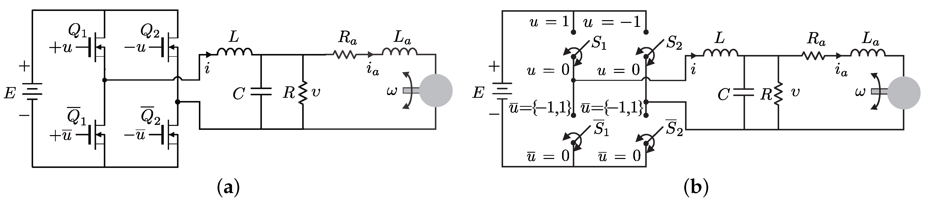
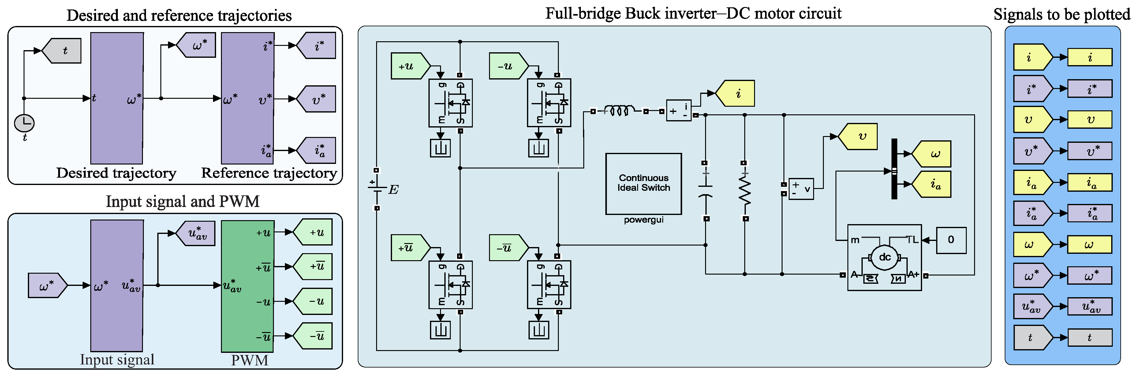
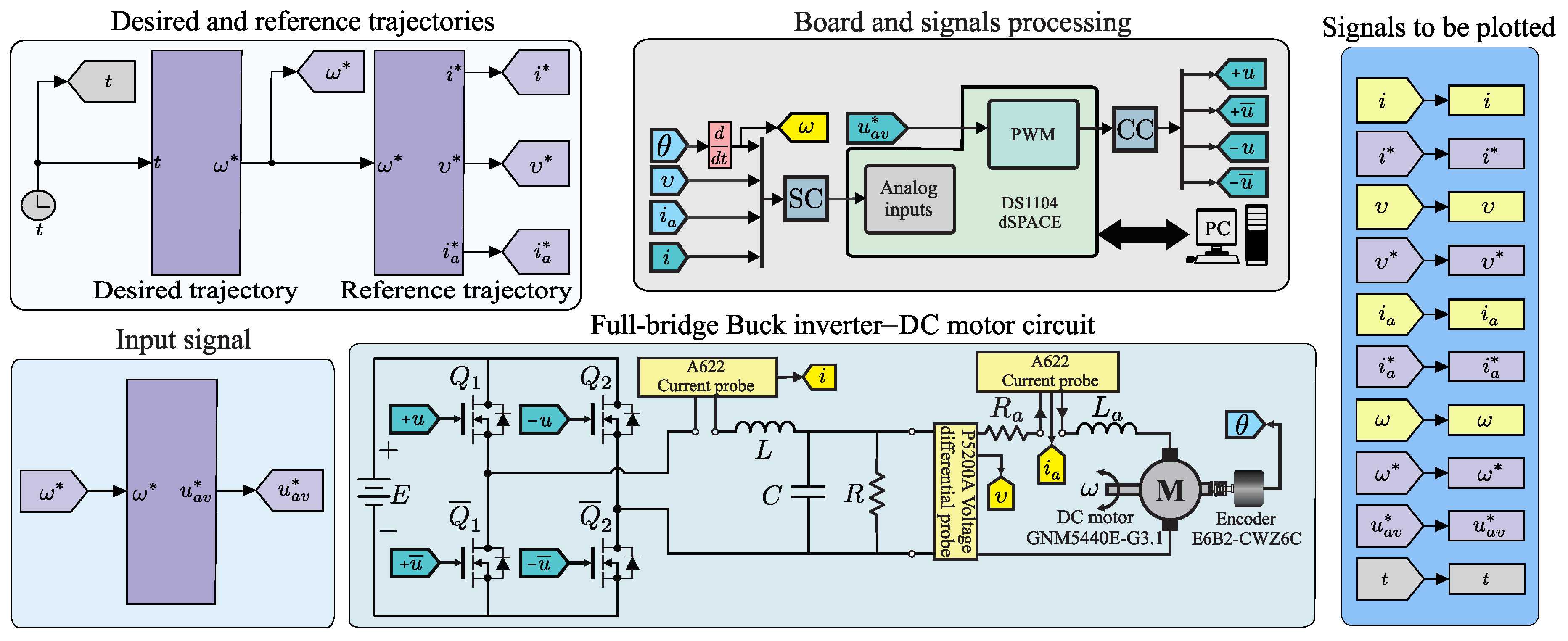
3.1.1. Connection Diagram of the System

The circuit simulation results are obtained through the diagram of the system shown in Figure 4, whose implementation has been executed via the SimPowerSystems toolbox of Matlab-Simulink. The blocks composing the diagram of this figure are detailed below:

• Desired and reference trajectories. In this block, the desired trajectory ${\omega }^{\ast }$ and the differential parametrization, see Equations (31)–(33), are programmed to obtain the reference trajectories $i_a^{\ast }$, ${\upsilon }^{\ast }$, and $i^{\ast }$.
• Signals to be plotted. The variables to be plotted are defined in this block. These variables are related to the full-bridge Buck inverter–DC motor system and to the differential parametrization.
• Input signal and PWM. Here, the input $u_{av}^{\ast }$, given by Equation (37), is programmed. Also, through this block, the full-bridge transistors are driven when the switched inputs are generated through the PWM signal.
• Full-bridge Buck inverter–DC motor circuit. This block corresponds to the overall system. The parameters of the full-bridge Buck inverter are given by the following values:

  $$\begin{array}{c}R=48\mathsf{\Omega },C=4.7\mathsf{\mu }\mathrm{F},L=4.94\mathrm{mH},E=32\mathrm{V}.\end{array}$$

  (47)
  The sampling frequency of the four transistors, associated with the full-bridge is 50 kHz. The DC motor was manufactured by ENGEL with a 3.1 gearbox with reduction ratio of 14.5:1. Such a motor is a GNM5440E-G3.1 $(24\mathrm{V},95\mathrm{W})$, whose parameters are

  $$\begin{array}{c}{L}_a=2.22\mathrm{mH},k_m=120.1\times {10}^{-3}\frac{\mathrm{N}·\mathrm{m}}{\mathrm{A}},\\ R_a=0.965\mathsf{\Omega },k_e=120.1\times {10}^{-3}\frac{\mathrm{V}·\mathrm{s}}{\mathrm{rad}},\\ J=118.2\times {10}^{-3}\mathrm{kg}·{\mathrm{m}}^2,b=129.6\times {10}^{-3}\frac{\mathrm{N}·\mathrm{m}·\mathrm{s}}{\mathrm{rad}}.\end{array}$$

  (48)

3.1.2. Circuit Simulation Results

With the intention of validating the obtained mathematical model of the full-bridge Buck inverter–DC motor system, this section presents the circuit simulation results for different desired trajectories of the angular velocity.

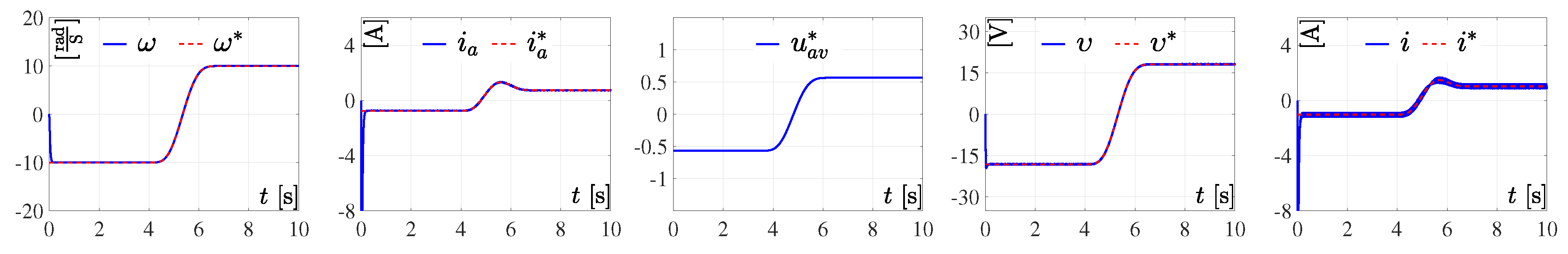
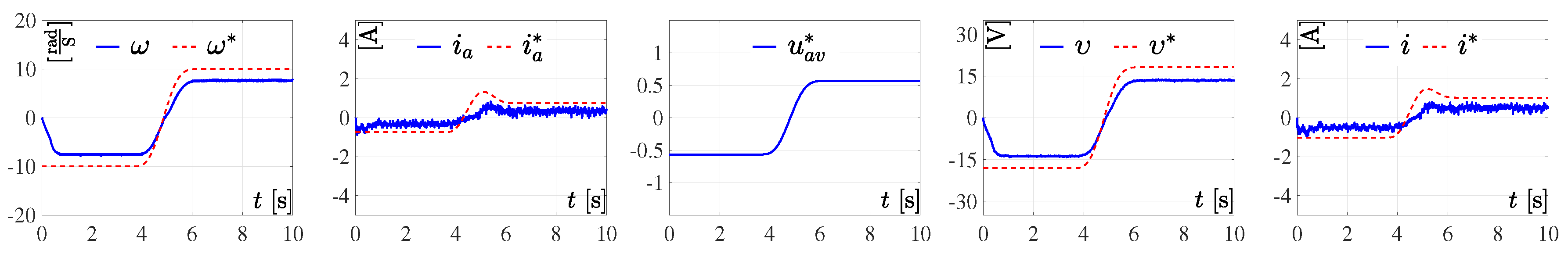
• Circuit Simulation 1

In this simulation, the desired trajectory ${\omega }^{\ast }$ is generated via the following Bézier polynomial:

$$\begin{array}{c}\hfill {\omega }^{\ast }\left(t\right)={\overline{\omega }}_i\left(t_i\right)+[{\overline{\omega }}_f\left(t_f\right)-{\overline{\omega }}_i\left(t_i\right)]\phi (t,t_i,t_f),\end{array}$$

(49)

where $\phi (t,t_i,t_f)$ is given by

$$\begin{array}{c}\hfill \phi \left(t,t_i,t_f\right)=\left\{\begin{array}{c}0\mathrm{for}t\le t_i,\hfill \\ {\left(\frac{t-t_i}{t_f-t_i}\right)}^5\times \left[\phantom{{\left(\frac{t-t_i}{t_f-t_i}\right)}^5}{r}_1+r_2\left(\frac{t-t_i}{t_f-t_i}\right)\right.+r_3{\left(\frac{t-t_i}{t_f-t_i}\right)}^2\hfill \\ +r_4{\left(\frac{t-t_i}{t_f-t_i}\right)}^3+r_5{\left(\frac{t-t_i}{t_f-t_i}\right)}^4\left.+r_6{\left(\frac{t-t_i}{t_f-t_i}\right)}^5\right]\mathrm{for}t\in (t_i,t_f),\hfill \\ 1\mathrm{for}t\ge t_f,\hfill \end{array}\right.\end{array}$$

(50)

and

$$r_1=252,r_2=-1050,r_3=1800,r_4=-1575,r_5=700,r_6=-126.$$

(51)

With proposal (50) and coefficients (51), ${\omega }^{\ast }$ smoothly interpolates between ${\overline{\omega }}_i=-10\frac{\mathrm{rad}}{\mathrm{s}}$ and ${\overline{\omega }}_f=10\frac{\mathrm{rad}}{\mathrm{s}}$ over the time interval $[t_i,t_f]=[4\mathrm{s},6\mathrm{s}]$. Note that if (50) were of different order, then coefficients (51) would be also different. The corresponding results are presented in Figure 5.

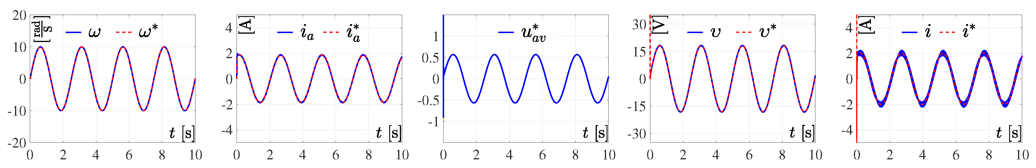
• Circuit Simulation 2

Here, ${\omega }^{\ast }$ is defined by the following sinusoidal function:

$$\begin{array}{c}\hfill {\omega }^{\ast }\left(t\right)=10\sin \left(0.8\pi t\right).\end{array}$$

(52)

Figure 6 depicts the corresponding simulation results.

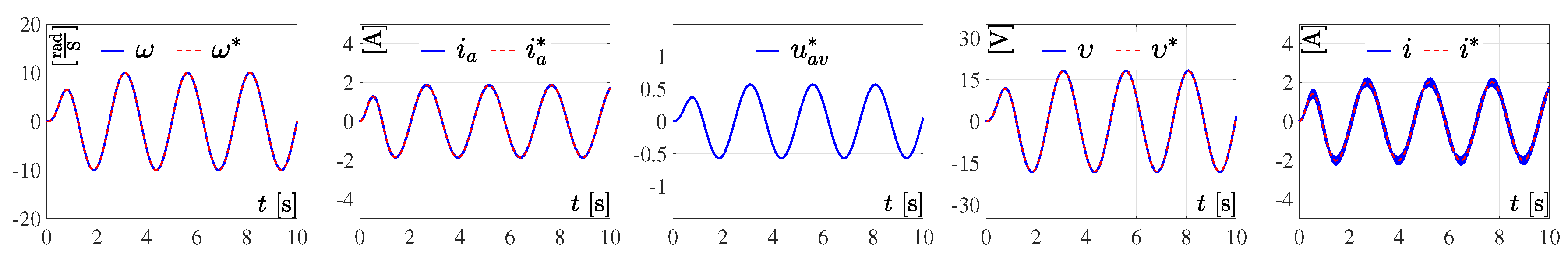
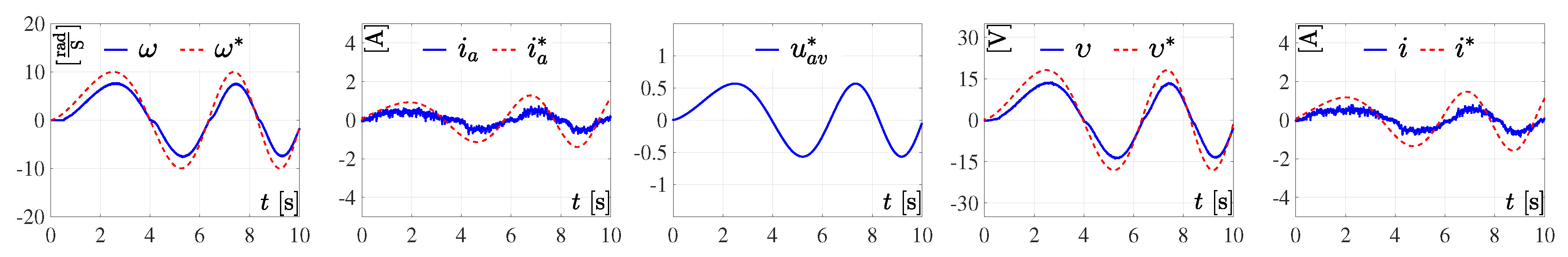
• Circuit Simulation 3

In this case, the trajectory to be tracked has been proposed as

$$\begin{array}{c}\hfill {\omega }^{\ast }\left(t\right)=10\left(1-e^{-2t^2}\right)\sin \left(0.8\pi t\right),\end{array}$$

(53)

and the results are shown in Figure 7.

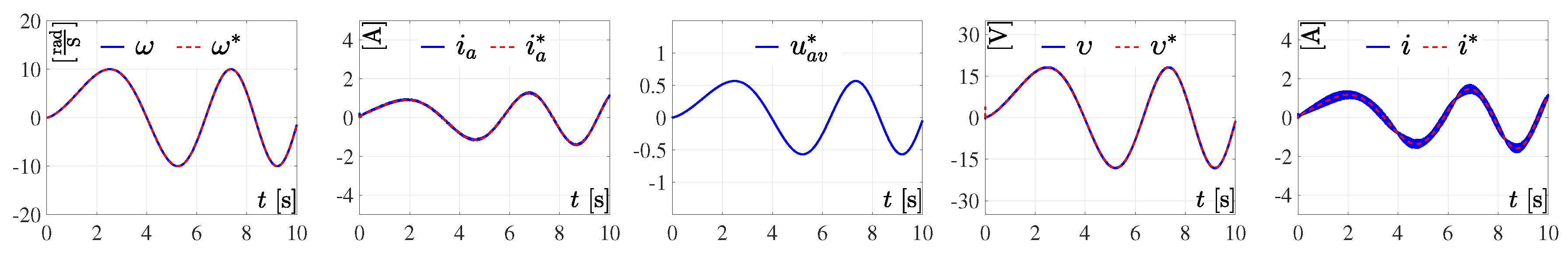
• Circuit Simulation 4

Lastly, the trajectory to be tracked in this simulation is given by Equation (54) and the corresponding results are presented in Figure 8.

$$\begin{array}{c}\hfill {\omega }^{\ast }\left(t\right)=10\sin \left(0.125\pi t^{\frac{3}{2}}\right).\end{array}$$

(54)

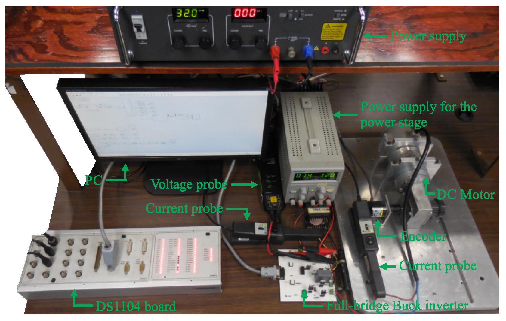
3.2. Results from the Experimental Prototype

This section describes the connection diagram that allows the implementation of the input signal $u_{av}^{\ast }$ on the built prototype of the full-bridge Buck inverter–DC motor system shown in Figure 9. Also, the corresponding experimental results are presented.

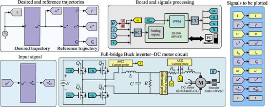
3.2.1. Experimental Diagram of the System

The experimental results were obtained by using the connection diagram depicted in Figure 10. The blocks composing this figure are described below.

• Desired and reference trajectories. The desired trajectory ${\omega }^{\ast }$ and the Equations (31)–(33) to obtain the reference trajectories $i_a^{\ast }$, ${\upsilon }^{\ast }$, and $i^{\ast }$ are programmed in this block.
• Input signal. The input $u_{av}^{\ast }$, see Equation (37), is programmed here.
• Signals to be plotted. The variables to be plotted are specified in this block.
• Board and signal processing. This block shows the connections between the DS1104 board and the system. As can be seen, signal conditioning (SC) is executed over the angular position $\theta$, the voltage $\upsilon$, and the currents $i_a$ and i. Also, the input signal $u_{av}^{\ast }$ is introduced into the DS1104 board so that the PWM signal can be generated. This latter is processed through the sub-block conditioning circuit (CC) allowing the correct activation of the transistors.
• Full-bridge Buck inverter–DC motor circuit. This block corresponds to the system under study and the values of its parameters were defined in (47). The sampling frequency of the four IRF640 MOSFET transistors associated with the full-bridge is 50 kHz. Additionally, the parameters of the DC motor are the same of those considered in (48).

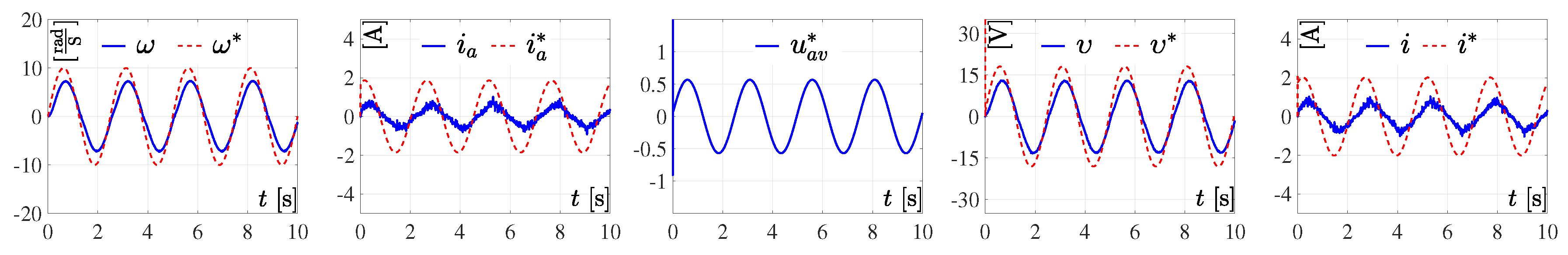
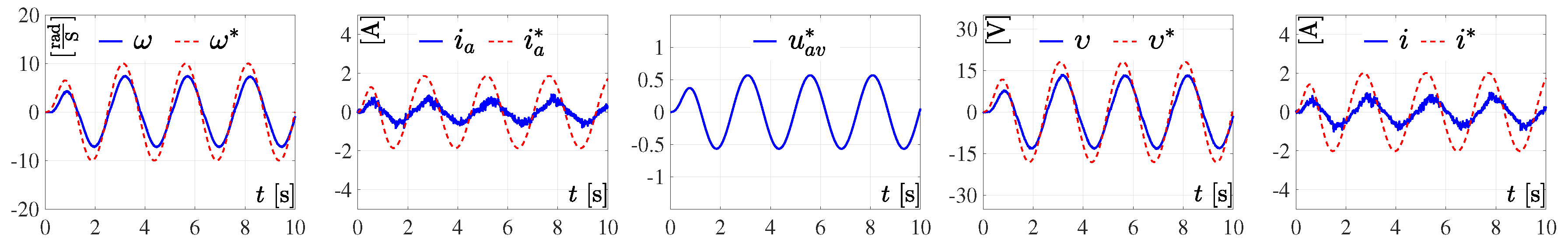
3.2.2. Experimental Results

With the purpose of validating the obtained mathematical model (21)–(24), this section presents the experimental results for the system. In these experiments, and with the purpose of making a fair comparison with the simulation results, the desired trajectories for $\omega$ are the same as those considered in the simulation results.

• Experiment 1

In this experiment, ${\omega }^{\ast }$ is the Bézier-type trajectory defined in (49). The experimental results of the system are presented in Figure 11.

• Experiment 2

Here, ${\omega }^{\ast }$ is the sinusoidal trajectory (52). In Figure 12, the corresponding experimental results are depicted.

• Experiment 3

In this experiment, the desired angular velocity is defined as in (53). The corresponding experimental results are shown in Figure 13.

• Experiment 4

Lastly, Figure 14 presents the experimental result associated with Equation (54).

4. Discussion

As the mathematical model developed herein for the full-bridge Buck inverter–DC motor system was differentially flat, all system variables were parameterized in terms of the flat output. Later, by proposing and replacing ${\omega }^{\ast }$ into the differential parametrization of the system, the reference variables ($i_a^{\ast }$, $i^{\ast }$, ${\upsilon }^{\ast }$) and the input signal ($u_{av}^{\ast }$) were found offline. This was made to compare the results of the circuit simulation with the differential parametrization results, both shown in Figure 5, Figure 6, Figure 7 and Figure 8. The same thing was done in order to compare the experimental results and the differential parametrization results, both shown in Figure 11, Figure 12, Figure 13 and Figure 14. Regarding these latter, a tracking error between system variables $\omega$, $i_a$, $\upsilon$, i and reference variables ${\omega }^{\ast }$, $i_a^{\ast }$, ${\upsilon }^{\ast }$, $i^{\ast }$ can be observed. Such an error appears because some dynamics were not included into the mathematical model, i.e., energy losses associated with semiconductors and parasitic resistances related to capacitor and inductors. In this sense, note that, due to these omitted dynamics and the existence of the load R, the efficiency of the Buck converter is $89.14\%$. On the other hand, if all the neglected dynamics were taken into account, then the mathematical model would be more complex and this is far beyond the scope of this paper. In brief, the obtained results depicted in Figure 5, Figure 6, Figure 7 and Figure 8 and Figure 11, Figure 12, Figure 13 and Figure 14 validate the good accuracy of the proposed mathematical model.

5. Conclusions

With the aim of validating, through circuit simulations and experimental results, the proposed mathematical model of the new “full-bridge Buck inverter–DC motor” system, the flatness property has been exploited. Likewise, the steady-state, stability, and controllability properties associated with the dynamic behavior of such a system have been developed.

In the development of the mathematical model of the new “full-bridge Buck inverter–DC motor” system, all components were considered as ideal. This was done with the intention of obtaining a non-complex mathematical model that would still enjoy relatively good accuracy. On the other hand, by applying the flatness concept to the proposed mathematical model, it was found that the flat output of the system is given by $\omega$. Therefore, the vector state and the input signal were differentially parameterized, in terms of the flat output and its successive derivatives with respect to time. Thus, with the help of such a parametrization, the validation of the deduced mathematical model was carried out through circuit simulation and a built prototype of the system. The circuit simulation results (presented in Figure 5, Figure 6, Figure 7 and Figure 8) and the experimental results (depicted in Figure 11, Figure 12, Figure 13 and Figure 14) validates the proposed mathematical model despite the small tracking error between system variables and reference variables. It is worth mentioning that such an error could be minimized if the electronic and electric elements were considered nonideal, meaning that energy losses and parasitic resistances should be considered into the mathematical model. However, the advantages of using the model presented in this paper is its simplicity and its accuracy.

Future research will be devoted to the design of feedback tracking controls and their experimental implementation on the prototype of the system that has been built.

References

1. Lyshevski, S.E. Electromechanical Systems, Electric Machines, and Applied Mechatronics; CRC Press: Boca Raton, FL, USA, 2000; ISBN 0-8493-2275-8. [Google Scholar]
2. Ahmad, M.A.; Ismail, R.M.T.R.; Ramli, M.S. Control strategy of Buck converter driven DC motor: A comparative assessment. Austral. J. Basic Appl. Sci. 2010, 4, 4893–4903. [Google Scholar]
3. Bingöl, O.; Paçaci, S. A virtual laboratory for neural network controlled DC motors based on a DC-DC Buck converter. Int. J. Eng. Educ. 2012, 28, 713–723. [Google Scholar]
4. Sira-Ramírez, H.; Oliver-Salazar, M.A. On the robust control of Buck-converter DC-motor combinations. IEEE Trans. Power Electron. 2013, 28, 3912–3922. [Google Scholar] [CrossRef]
5. Silva-Ortigoza, R.; García-Sánchez, J.R.; Alba-Martínez, J.M.; Hernández-Guzmán, V.M.; Marcelino-Aranda, M.; Taud, H.; Bautista-Quintero, R. Two-stage control design of a Buck converter/DC motor system without velocity measurements via a Σ-Δ-modulator. Math. Probl. Eng. 2013, 2013, 929316. [Google Scholar] [CrossRef]
6. Hoyos, F.E.; Rincón, A.; Taborda, J.A.; Toro, N.; Angulo, F. Adaptive quasi-sliding mode control for permanent magnet DC motor. Math. Probl. Eng. 2013, 2013, 693685. [Google Scholar] [CrossRef]
7. Silva-Ortigoza, R.; Márquez-Sánchez, C.; Carrizosa-Corral, F.; Antonio-Cruz, M.; Alba-Martínez, J.M.; Saldaña-González, G. Hierarchical velocity control based on differential flatness for a DC/DC Buck converter-DC motor system. Math. Probl. Eng. 2014, 2014, 912815. [Google Scholar] [CrossRef]
8. Wei, F.; Yang, P.; Li, W. Robust adaptive control of DC motor system fed by Buck converter. Int. J. Control Autom. 2014, 7, 179–190. [Google Scholar] [CrossRef]
9. Silva-Ortigoza, R.; Hernández-Guzmán, V.M.; Antonio-Cruz, M.; Muñoz-Carrillo, D. DC/DC Buck power converter as a smooth starter for a DC motor based on a hierarchical control. IEEE Trans. Power Electron. 2015, 30, 1076–1084. [Google Scholar] [CrossRef]
10. Hernández-Guzmán, V.M.; Silva-Ortigoza, R.; Muñoz-Carrillo, D. Velocity control of a brushed DC-motor driven by a DC to DC Buck power converter. Int. J. Innov. Comp. Inf. Control 2015, 11, 509–521. [Google Scholar]
11. Kumar, S.G.; Thilagar, S.H. Sensorless load torque estimation and passivity based control of Buck converter fed DC motor. Sci. World J. 2015, 2015, 132843. [Google Scholar] [CrossRef]
12. Khubalkar, S.; Chopade, A.; Junghare, A.; Aware, M.; Das, S. Design and realization of stand-alone digital fractional order PID controller for Buck converter fed DC motor. Circuits Syst. Signal Process. 2016, 35, 2189–2211. [Google Scholar] [CrossRef]
13. Rigatos, G.; Siano, P.; Wira, P.; Sayed-Mouchaweh, M. Control of DC–DC converter and DC motor dynamics using differential flatness theory. Intell. Ind. Syst. 2016, 2, 371–380. [Google Scholar] [CrossRef]
14. Nizami, T.K.; Chakravarty, A.; Mahanta, C. Design and implementation of a neuro-adaptive backstepping controller for Buck converter fed PMDC-motor. Control Eng. Pract. 2017, 58, 78–87. [Google Scholar] [CrossRef]
15. Hoyos Velasco, F.E.; Candelo-Becerra, J.E.; Rincón Santamaria, A. Dynamic analysis of a permanent magnet DC motor using a Buck converter controlled by ZAD-FPIC. Energies 2018, 11, 3388. [Google Scholar] [CrossRef]
16. Khubalkar, S.W.; Junghare, A.S.; Aware, M.V.; Chopade, A.S.; Das, S. Demonstrative fractional order-PID controller based DC motor drive on digital platform. ISA Trans. 2018, 82, 79–93. [Google Scholar] [CrossRef]
17. Rigatos, G.; Siano, P.; Ademi, S.; Wira, P. Flatness-based control of DC-DC converters implemented in successive loops. Electr. Power Compon. Syst. 2018, 46, 673–687. [Google Scholar] [CrossRef]
18. Yang, J.; Wu, H.; Hu, L.; Li, S. Robust predictive speed regulation of converter-driven DC motors via a discrete-time reduced-order GPIO. IEEE Trans. Ind. Electron. 2019, 66, 7893–7903. [Google Scholar] [CrossRef]
19. Rigatos, G.; Siano, P.; Sayed-Mouchaweh, M. Adaptive neurofuzzy H-infinity control of DC-DC voltage converters. Neural Comput. Appl. 2019, 1–14. [Google Scholar] [CrossRef]
20. Ismail, A.A.A.; Elnady, A. Advanced drive system for DC motor using multilevel DC/DC Buck converter circuit. IEEE Access 2019, 7, 54167–54178. [Google Scholar] [CrossRef]
21. Silva-Ortigoza, R.; Alba-Juárez, J.N.; García-Sánchez, J.R.; Antonio-Cruz, M.; Hernández-Guzmán, V.M.; Taud, H. Modeling and experimental validation of a bidirectional DC/DC Buck power electronic converter–DC motor system. IEEE Latin Am. Trans. 2017, 15, 1043–1051. [Google Scholar] [CrossRef]
22. Silva-Ortigoza, R.; Alba-Juárez, J.N.; García-Sánchez, J.R.; Hernández-Guzmán, V.M.; Sosa-Cervantes, C.Y.; Taud, H. A sensorless passivity-based control for the DC/DC Buck converter–inverter–DC motor system. IEEE Latin Am. Trans. 2016, 14, 4227–4234. [Google Scholar] [CrossRef]
23. Hernández-Márquez, E.; García-Sánchez, J.R.; Silva-Ortigoza, R.; Antonio-Cruz, M.; Hernández-Guzmán, V.M.; Taud, H.; Marcelino-Aranda, M. Bidirectional tracking robust controls for a DC/DC Buck converter-DC motor system. Complexity 2018, 2018, 1260743. [Google Scholar] [CrossRef]
24. Linares-Flores, J.; Reger, J.; Sira-Ramírez, H. Load torque estimation and passivity-based control of a Boost-converter/DC-motor combination. IEEE Trans. Control Syst. Technol. 2010, 18, 1398–1405. [Google Scholar] [CrossRef]
25. García-Rodríguez, V.H.; Silva-Ortigoza, R.; Hernández-Márquez, E.; García-Sánchez, J.R.; Taud, H. DC/DC Boost converter–inverter as driver for a DC motor: Modeling and experimental verification. Energies 2018, 11, 2044. [Google Scholar] [CrossRef]
26. García-Sánchez, J.R.; Hernández-Márquez, E.; Ramírez-Morales, J.; Marciano-Melchor, M.; Marcelino-Aranda, M.; Taud, H.; Silva-Ortigoza, R. A robust differential flatness-based tracking control for the “MIMO DC/DC Boost converter–inverter–DC motor” system: Experimental results. IEEE Access 2019, 7, 84497–84505. [Google Scholar] [CrossRef]
27. Linares-Flores, J.; Barahona-Avalos, J.L.; Sira-Ramírez, H.; Contreras-Ordaz, M.A. Robust passivity-based control of a Buck–Boost-converter/DC-motor system: An active disturbance rejection approach. IEEE Trans. Ind. Appl. 2012, 48, 2362–2371. [Google Scholar] [CrossRef]
28. Hernández-Márquez, E.; Silva-Ortigoza, R.; García-Sánchez, J.R.; Marcelino-Aranda, M.; Saldaña-González, G. A DC/DC Buck-Boost converter–inverter–DC motor system: Sensorless passivity-based control. IEEE Access 2018, 6, 31486–31492. [Google Scholar] [CrossRef]
29. Hernández-Márquez, E.; Avila-Rea, C.A.; García-Sánchez, J.R.; Silva-Ortigoza, R.; Silva-Ortigoza, G.; Taud, H.; Marcelino-Aranda, M. Robust tracking controller for a DC/DC Buck-Boost converter–inverter–DC motor system. Energies 2018, 11, 2500. [Google Scholar] [CrossRef]
30. Ghazali, M.R.; Ahmad, M.A.; Ismail, R.M.T.R. Adaptive safe experimentation dynamics for data-driven neuroendocrine-PID control of MIMO systems. IETE J. Res. 2019, 1–14. [Google Scholar] [CrossRef]
31. Sira-Ramírez, H.; Pérez-Moreno, R.A.; Ortega, R.; García-Esteban, M. Passivity-based controllers for the stabilization of DC-to-DC power converters. Automatica 1997, 33, 499–513. [Google Scholar] [CrossRef]
32. Hernández-Márquez, E.; Avila-Rea, C.A.; Silva-Ortigoza, R.; García-Sánchez, J.R.; Antonio-Cruz, M.; Taud, H.; Marcelino-Aranda, M. Modeling and simulation of a DC motor fed by a full-bridge Buck inverter. In Proceedings of the 2017 International Conference on Mechatronics, Electronics and Automotive Engineering, ICMEAE 2017, Cuernavaca, Mexico, 21–24 November 2017; pp. 77–81. [Google Scholar]
33. Sira-Ramírez, H.; Agrawal, S.K. Differentially Flat Systems; Marcel Dekker: New York, NY, USA, 2004; ISBN 0-8247-5470-0. [Google Scholar]
34. Hernández-Guzmán, V.M.; Silva-Ortigoza, R. Velocity Control of a Permanent Magnet Brushed Direct Current Motor. In Automatic Control with Experiments. Advanced Textbooks in Control and Signal Processing; Springer: Cham, Switzerland, 2019; pp. 605–644. ISBN 978-3-319-75804-6. [Google Scholar] [CrossRef]
35. Usman, H.M.; Mukhopadhyay, S.; Rehman, H. Permanent magnet DC motor parameters estimation via universal adaptive stabilization. Control Eng. Pract. 2019, 90, 50–62. [Google Scholar] [CrossRef]
Figure 1. The full-bridge Buck inverter–DC motor topology: (a) proposed structure and (b) ideal configuration.
Electronics 08 01216 g001
Figure 2. The full-bridge Buck inverter–DC motor system: (a) ideal circuit for positive cycle; (b) in positive cycle Q 1 and Q ¯ 1 of Figure 1 operate as a transistor and as a diode, respectively; (c) energy charging mode of operation; and (d) energy discharging mode of operation.
Electronics 08 01216 g002
Figure 3. The full-bridge Buck inverter–DC motor system: (a) ideal circuit for negative cycle; (b) in negative cycle Q 2 and Q ¯ 2 of Figure 1 operate as a transistor and as a diode, respectively; (c) energy charging mode of operation; and (d) energy discharging mode of operation.
Electronics 08 01216 g003
Figure 4. Circuit of the “full-bridge Buck inverter–DC motor” system designed via the SimPowerSystems toolbox of Matlab-Simulink. This circuit is used for validating the deduced mathematical model of such a system.
Electronics 08 01216 g004
Figure 5. Circuit simulation results for a Bézier polynomial-type trajectory. The results related to the mathematical model are denoted by ω , i a , υ , i, and the results associated with the reference variables are labeled as ω , i a , u a v , υ , i .
Electronics 08 01216 g005
Figure 6. Circuit simulation results for a sinusoidal trajectory. The results of the mathematical model correspond to variables ω , i a , υ , i, whereas the results related to the reference variables are ω , i a , u a v , υ , i .
Electronics 08 01216 g006
Figure 7. Circuit simulation results for a sinusoidal trajectory with exponential amplitude. The results associated with the mathematical model are ω , i a , υ , i, and the results of the reference variables correspond to ω , i a , u a v , υ , i .
Electronics 08 01216 g007
Figure 8. Circuit simulation results for a sinusoidal trajectory with time-varying frequency. The results related to the mathematical model correspond to the signals denoted by ω , i a , υ , i, and the results associated with the reference variables are labeled as ω , i a , u a v , υ , i .
Electronics 08 01216 g008
Figure 9. Experimental prototype of the full-bridge Buck inverter–DC motor system.
Electronics 08 01216 g009
Figure 10. Experimental diagram of the “full-bridge Buck inverter–DC motor” system.
Electronics 08 01216 g010
Figure 11. Experimental results for a Bézier-type trajectory. The results of the measured variables are ω , i a , υ , i, and the results of the reference variables are ω , i a , u a v , υ , i .
Electronics 08 01216 g011
Figure 12. Experimental results for a sinusoidal trajectory. The results related to the measured variables correspond to the signals denoted by ω , i a , υ , i, whereas the results associated with the reference variables are labeled as ω , i a , u a v , υ , i .
Electronics 08 01216 g012
Figure 13. Experimental results for a sinusoidal trajectory with exponential amplitude. The results of the measured variables correspond to ω , i a , υ , i, and the results of the reference variables are ω , i a , u a v , υ , i .
Electronics 08 01216 g013
Figure 14. Experimental results for a sinusoidal trajectory with time-varying frequency. The results associated with the measured variables are denoted as ω , i a , υ , i, whereas the results related to the reference variables are labeled as ω , i a , u a v , υ , i .
Electronics 08 01216 g014