1. Introduction
In communication systems, signal-to-noise ratio (SNR) is a very important parameter, which characterizes channel quality. It is a priori information necessary for many signal processing algorithms or techniques, such as signal detection, power control, turbo decoding, adaptive modulation and demodulation, etc.
In general, according to the amount of knowledge available for a received signal, SNR estimators are classified into two types: a data-aid (DA) estimator and a non-data-aid (NDA) estimator. A DA estimator, such as maximum likelihood (ML) SNR estimator [
1,
2], Squared signal-to-noise variance (SNV) estimator [
3], can usually be used if the transmitted data or pilot symbols are fully known to the receiving side. In contrast, an NDA estimator, such as second and forth moment (M2M4) estimator [
4], split-symbol moment estimator (SSME) [
5] and signal-to-variation ratio (SVR) estimator [
6], can estimate the SNR solely from the unknown, information-bearing portion of the received signals. Although the performance of DA estimators may be better, NDA estimators do not invade on the throughput of the channel and require less a priori information. Therefore, NDA estimators are more practical, especially for non-cooperative scenarios.
During the last few decades, many SNR estimators have been proposed [
7,
8,
9,
10,
11,
12]. However, most of these SNR estimators still have the following limitations: (1) The application range of the modulation types is limited. For example, the ML SNR estimator is only applicable for BPSK signals, and M-ary PSK signals, and the M2M4 estimator is only applicable for MPSK signals. (2) The effective estimation range is narrow. For example, the performance of the subspace-based SNR estimation algorithms at low SNR is not ideal. The main reason is that the dimension of the signal subspace is easily overestimated under low SNR conditions. (3) Their robustness is poor. Many SNR estimators assume that the receiving system is perfectly synchronized, i.e., neither the timing offset nor the frequency offset exists. However, this requirement cannot always be met in the practical scenario, especially for non-cooperative scenarios.
On the other hand, many channel estimation methods based on deep learning (DL) have been proposed [
13,
14,
15]. Compared to traditional channel estimation techniques, the performance and robustness of DL-based channel estimation are better. Inspired by this, an SNR estimation method based on deep learning is proposed in this paper, which aims to improve the performance of current SNR estimation, especially for non-cooperative scenarios. In view of the fact that the estimated performance of the M2M4 estimator is superior and widely studied and applied, it is used as a benchmark for the DL-based SNR estimator proposed in this paper.
The main contributions of this paper are summarized as follows:
Firstly, based on the derivation of the ML SNR estimator, this paper expounds the reasons for using a deep convolutional neural network to estimate the SNR of the received signal. The DL-based SNR estimator proposed in this paper is an end-to-end SNR method. Different from the traditional SNR estimation method, this method does not need to manually design an SNR estimator, and minimizes the need for expert knowledge, which effectively improves the development speed of the SNR estimation system.
Secondly, in order to accommodate the varying input dimensions and avoid the training problem of deep neural network caused by long input signal, an SNR estimation strategy is carefully designed in this paper. Specifically, for a received signal to be estimated (the length of which is different from the input dimension of the trained deep neural network, which may be very large), we use the following strategy to estimate its SNR: first, splitting it so that the length of each segment is consistent with the input dimension of the deep neural network. Each segment is then fed into the trained deep neural network to obtain the output. Then, inputting each segment to the trained deep neural network to obtain its output. It is worth noting that the output of the deep neural network is not an estimate of the SNR, but an estimate of its amplitude. Finally, according to a certain method, the amplitude estimate of each segment is used to calculate the SNR estimate of the received signal with a large input dimension.
Finally, the DL-based SNR estimation method proposed in this paper is an NDA estimator. Compared with the traditional SNR estimation methods represented by M2M4 estimator, the performance and robustness of the proposed method are better, and the application range of modulation types is wider. At the same time, the proposed method is not only applicable to the baseband signal, but can also estimate the SNR of the intermediate frequency (IF) signal.
The rest of this paper is organized as follows: In
Section 2, the deep neural network used in this paper is introduced. Experiments and comparisons are shown in
Section 3. Finally,
Section 4 demonstrates the conclusions and discussions.
2. System Model
In this section, we first review the ML SNR estimator. Secondly, we briefly introduce the convolutional neural network. Then, based on the derivation of the ML SNR estimator, we explain the reasons for using a convolutional neural network to estimate the SNR of the received signal. Finally, we describe the proposed SNR estimation method.
2.1. ML SNR Estimator
The ML SNR estimator is optimal for the case of aid-data accessible, and it can be close to the Cramer-Rao lower bound. It is introduced by Kerr [
1] and Gagliardi and Tomas [
2].
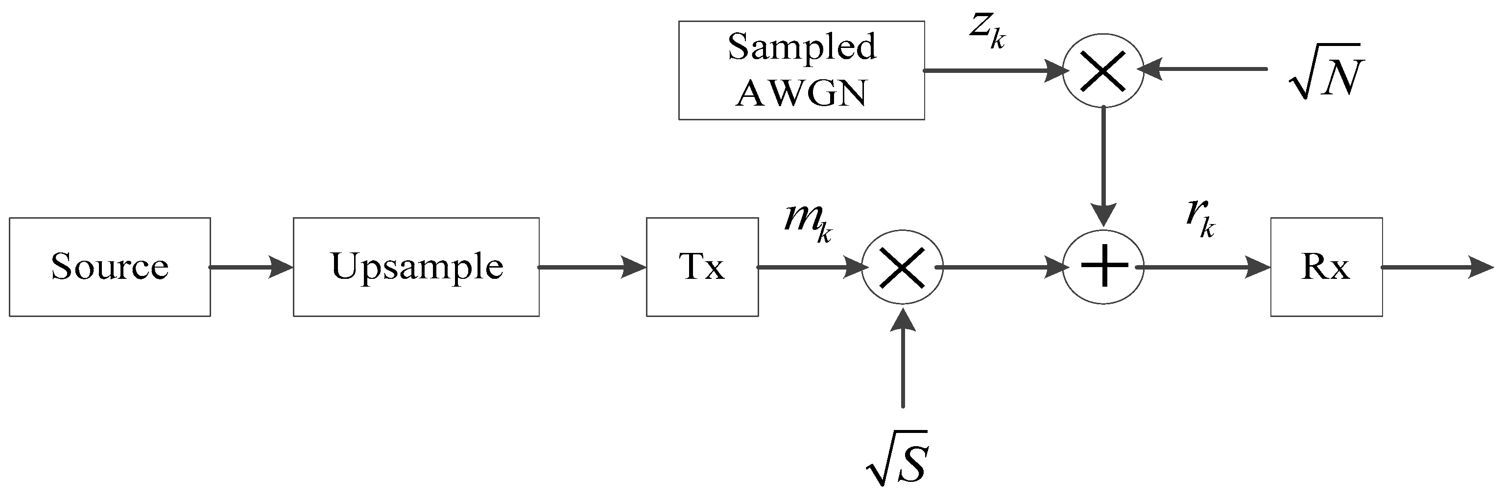
A complex, discrete, baseband-equivalent, band-limited model of coherent M-ary PSK in complex additive white Gaussian noise (AWGN) is shown in
Figure 1.
Assuming that the timing, phase, and frequency offsets do not exist, the received signal can be expressed as
where
is a sampled, pulsed-shaped information signal,
is a complex, sampled, zero-mean AWGN of unit variance,
is a signal power scale factor, and
is a noise power scale factor. Rewrite it in terms of real and imaginary parts as
Let
and
denote the in-phase and quadrature components of the noise, respectively, each of which is zero mean and variance
. Assuming that the in-phase and quadrature components of the noise are independent, their joint Probability Density Function (PDF) is
Using Equations (2) and (3), the joint PDF of the in-phase and quadrature components of the received signal sample can be written
the superscript
of
and
represents the
i-th transmission information sequence. Assuming that the signal and noise sequences are independent, then the joint PDF of the received sample with
points is (
is the number of source symbol and
is the number of samples per symbol)
Thus, the likelihood function
is
By solving the solution of the system of partial differential equations, and
, the estimated power
of signal and the estimated power
of noise are
Therefore, the ML SNR estimator of the received signal is
2.2. Convolutional Neural Networks
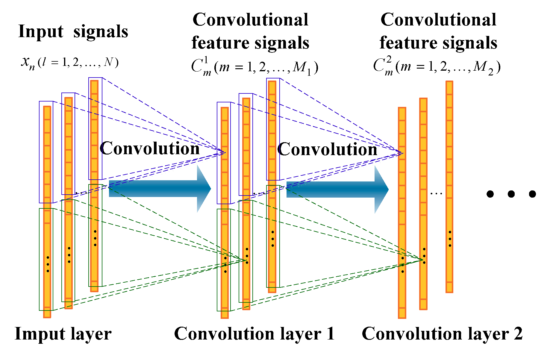
A one-dimensional (1D) convolutional neural network (part) is shown in
Figure 2. For the 1D convolution layer 1, the output
of the
-th filter is
where
represents the
-th column of the input of this convolution layer,
represents the
-th filter coefficient,
represents the bias of the
-th filter,
represents the convolution operation, and
represents the corresponding activation function. The activation function used in this paper is rectified linear unit (Relu):
.
For the 1D convolution layer 2, the output
of the
-th filter is
where
is the corresponding output of the previous layer. For example, if the previous layer is the convolution layer, then
.
Usually, the pooling layer is connected after the convolutional layer. The pooling layer is also a feature extraction process, which has the same number of feature signals (corresponding to the convolution kernel) as the convolution layer, except that the feature signal has a lower dimension. The purpose of the pooling operation is to reduce the dimension of the feature signals and enhance the invariance of the feature to deal with small disturbances. There are usually two pooling operations: maximum pooling and average pooling. When the maximum pooling function is applied, the pooling layer is defined as:
where
is the pooling size and
is the slide size, which determines the degree of overlap of the adjacent pool windows.
represents the
-th element of the
-th column of the output of this pooling layer. The reference [
16] claims that the performance of the maximum pooling is better than the average pooling. In the work of this paper, we employ the maximum pooling operation.
2.3. Reasons for Using CNN for SNR Estimation
Assuming that the channel environment is complex AWGN, and the timing, phase, and frequency offsets do not exist, then the samples of the received signal are independent identically distributed (IID). Therefore, the following two properties from Equation (6) need to be noticed:
The statistical properties of segment of length at arbitrary time intervals are the same, i.e., , where and represent the segments at different time intervals.
The signal sequence of length can be divided into consecutive subsequences, and the likelihood function can be expressed as , where .
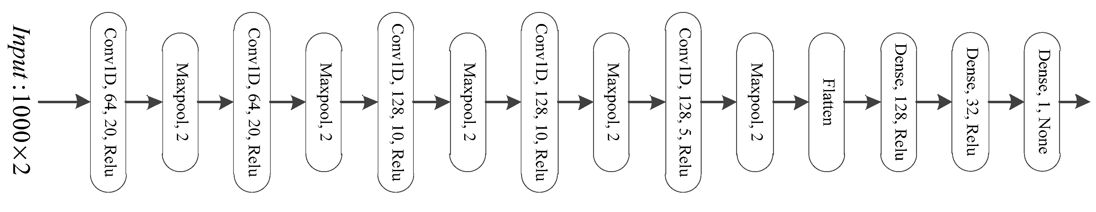
Property 1 indicates that the signals are identically distributed in the time domain. The signal segments at different time intervals have the same impulse response under the action of the convolution kernel, so features can be extracted at any time slot. Property 2 indicates that the likelihood function is compositional and can be approximated by a model of stacked cascade. Therefore, a CNN with a local perception domain will be more applicable than a fully-connected neural network, especially for large input dimensions CNN will be easier to train and the problem of overfitting will be lighter. Therefore, a deep (convolutional) neural network is used to estimate the SNR of the received signal in this paper and its structure is shown in
Figure 3. This deep neural network consists of five convolution layers, five maximum pooling layers, and three fully connected layers. Its parameters for each layer are shown in
Figure 3 (the structure of deep neural networks is one of the cores of deep learning based methods. However, the choice of the structure of the deep neural network is an open problem, usually heavily depending on the subjective experience of the researcher and certain experimental verification).
The input to the deep neural network is a raw signal vector. Before inputting this IQ signal
into the deep neural network, it is transformed as follows:
2.4. CNN-Based SNR Estimation
A longer input signal can make the SNR estimation of the target signal more accurate, while the requirements of different tasks also make the input dimension of the signal used to estimate its SNR variance. On the other hand, DL-based techniques have the following two limitations: Firstly, in general, the input dimension of the deep neural network must be clear before training and the input dimension for testing remains the same. Secondly, the longer input dimension means larger deep neural networks, which will result in easier overfitting and more computational resources and training samples needed.
In order to solve this contradiction, this paper estimates the signal amplitude of the target signal instead of directly estimating its SNR. In other words, the output of our deep neural network is not an estimate of the SNR of the received signal, but an estimate of its amplitude.
From Equation (7), the estimated amplitude
of the target signal is
Therefore, for a signal with a length of
, its estimated amplitude is
After obtaining the estimated amplitude of the received signal, its estimated SNR
is
Therefore, for each training batch, the loss function
of the deep neural network is
where
represents the signal amplitude of the
-th segment of the received signal,
represents the corresponding estimated value of
, and
is the parameter set of the deep neural network. This loss function will be minimized by adaptive moment (Adam) estimation, and the model parameter is updated iteratively as
where
denotes the learning rate. The problem of SNR estimation of the received signal with large input dimensions can be calculated by the following scheme:
Firstly, segmenting the received signal, the length of each segment is same as the input dimension of the deep neural network, denoted as .
Secondly, the signal amplitude of each segment is estimated by using the trained deep neural network.
Then, according to the estimated amplitude of each segment, the estimated amplitude of the target signal is obtained by using Equation (15).
Finally, the corresponding SNR of the received signal is calculated by using Equation (16).
3. Experiments
In this section, we will evaluate the performance of the DL-based SNR estimation method proposed in this paper. This paper focuses on the problem of SNR estimation under non-cooperative conditions. The M2M4 estimator, a widely used NDA estimator, will be used as the benchmark for the DL-based SNR estimator proposed in this paper.
For the received signal shown in Equation (2), assuming the signal and noise are zero-mean, independent random processes, and the in-phase and quadrature components of the noise are independent, then
where
is the second moment of the received signal,
is the forth moment of the received signal,
and
are the kurtosis of the target signal and noise, respectively. For any M-ary PSK signal,
, and for complex noise,
, so that
In this paper, simulation data generated by Matlab 2016b was used for experiments. The noise was a complex AWGN. The simulation data was first divided into three parts: the training data set, the validation data set, and the test data set. The deep neural network was trained according to Equation (18) by using the training data set. After each epoch training was completed, the validation data set was tested, and the deep neural network whose loss function value is minimal was saved as the optimal model. After completing all epochs’ training sessions, the test data set was used to evaluate the estimated performance of the deep learning based SNR estimator. The SNR of each training segment data was subjected to a uniform distribution of −40 dB–40 dB. The number of training data samples was 369,000, the number of validation data samples was 41,000, the epoch number was 150, and the batch size was 64. The early-stop training strategy was adopted and the optimizer used Adaptive moment estimation (Adam). The number of test data samples used to evaluate the performance was 410,000. All samples were normalized to zero mean with a unit variance, and its length was 1000.
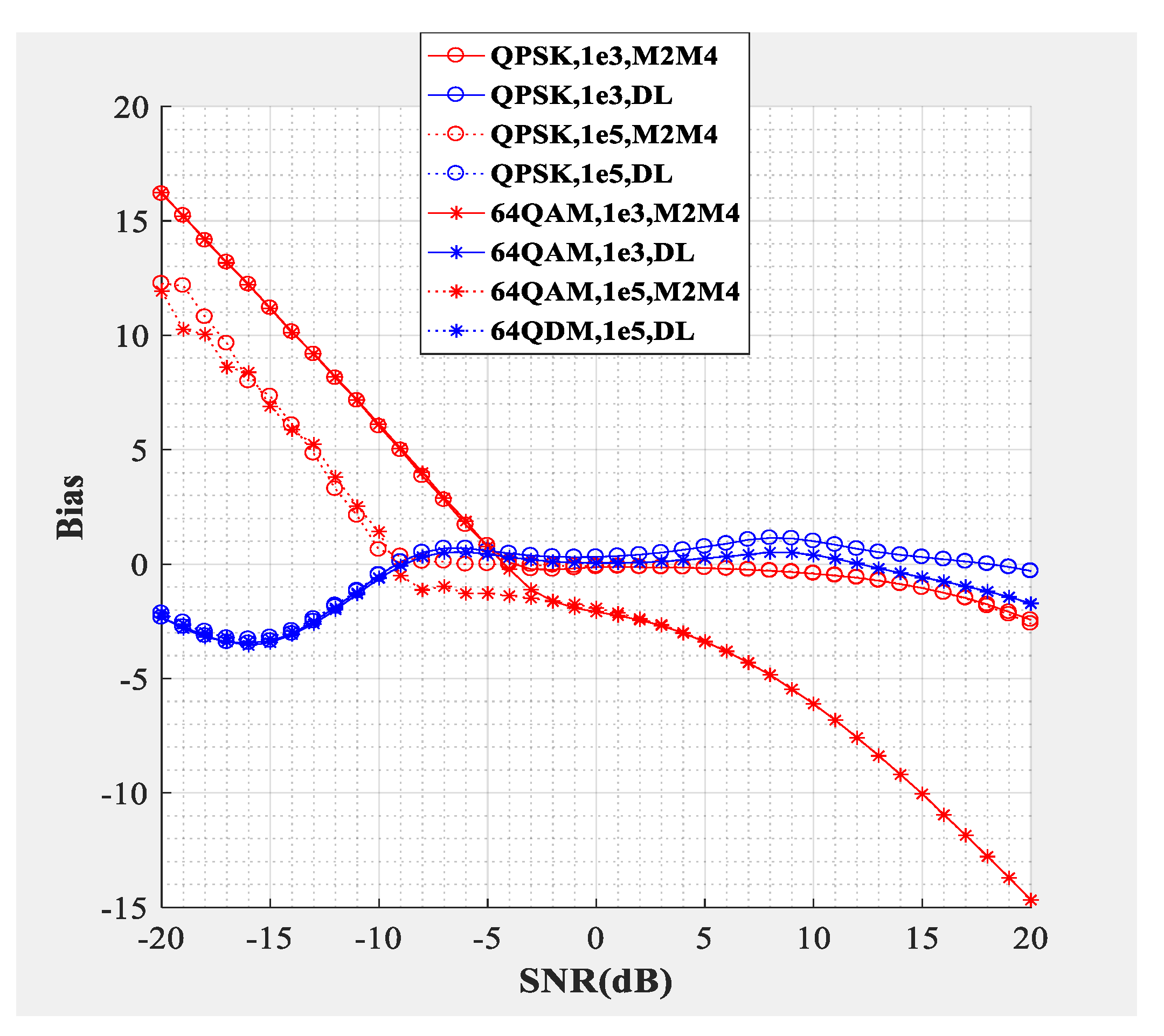
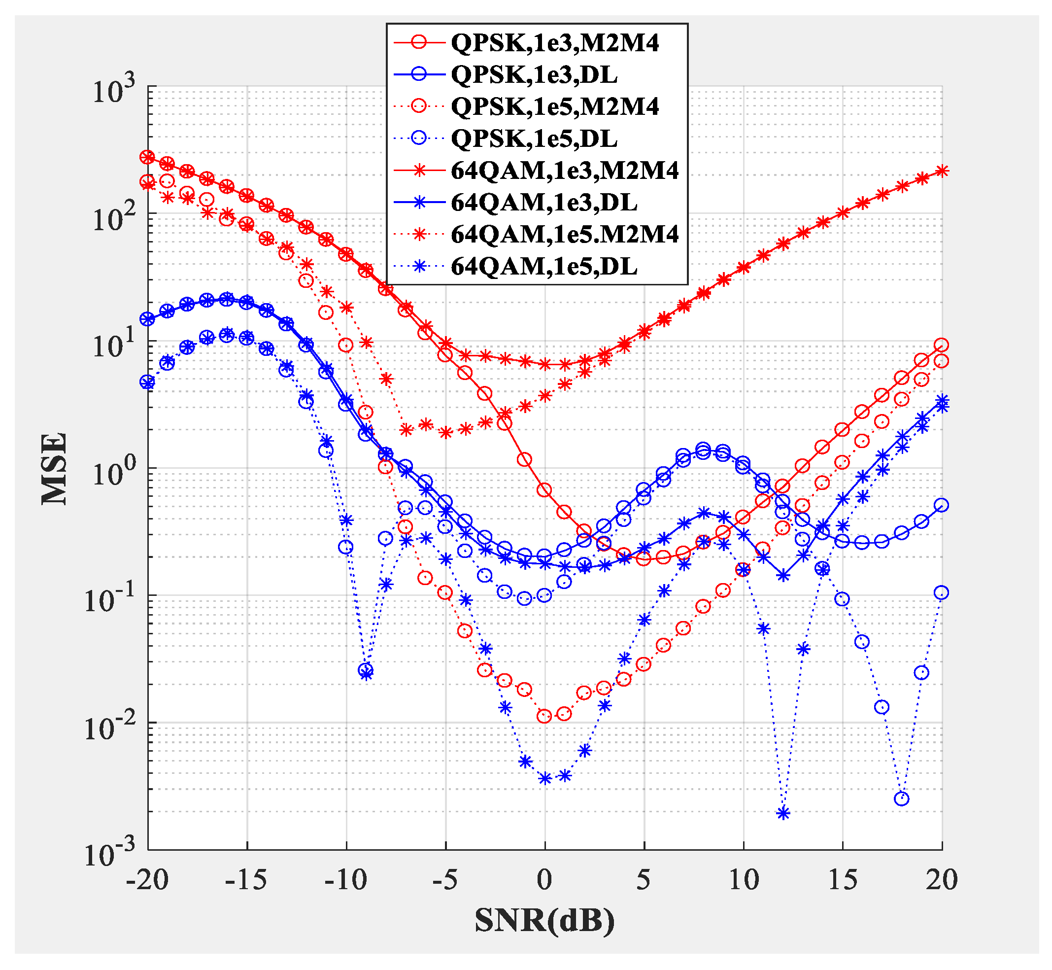
Figure 4;
Figure 5 compare the SNR estimation performance of the DL-based estimator and M2M4 estimator for baseband signal. The test dataset was baseband signal and the modulation types were QPSK and 64QAM (differentiated by different marks), the number of samples per symbol was
. The blue line represents the SNR estimation method proposed in this paper, and the red line represents the M2M4 estimator. The solid line represents that the dimension of the input signal was 1000 and the dotted line represents that the dimension of the input signal was 100,000. From the bias shown in
Figure 4 and the mean square error (MSE) shown in
Figure 5, the following conclusions can be drawn: Firstly, the SNR estimation performance of the method proposed in this paper is comparable to the M2M4 estimator for QPSK, but is superior to the M2M4 estimator for 64QAM. Secondly, longer input signal makes the MSE less, but does not affect the bias for the DL-based SNR estimator. Thirdly, for an SNR larger than 11 dB and less than −6 dB, the DL-based SNR estimator is superior to the M2M4 estimator.
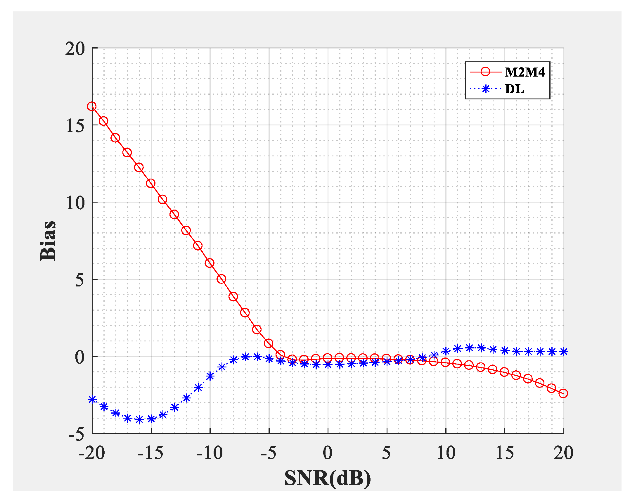
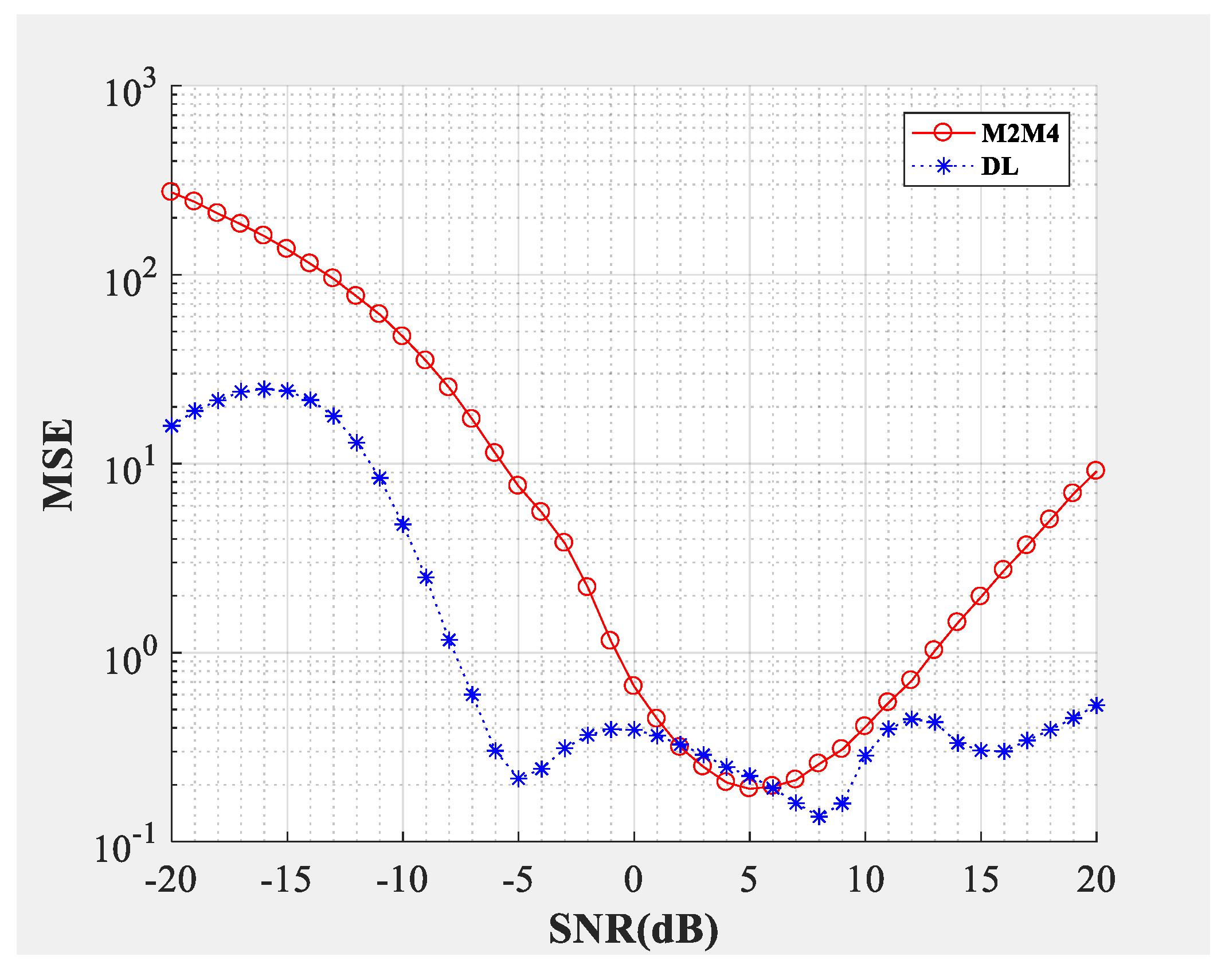
Figure 6 and
Figure 7 compare the estimation performance of the DL-based estimator and the M2M4 estimator for incoherent environments, i.e., phase offset or frequency offset exists (the random phase offset
and frequency offset
were added to each training segment’s data. The phase offset was subjected to a uniform distribution of 0°–10°, and the frequency offset was subjected to a uniform distribution of 0 Hz–120 Hz). The test dataset was baseband signal and the modulation type was QPSK. The number of samples per symbol was
. The phase offset value of 30° and the frequency offset value of 1000 Hz were tested. From the bias shown in
Figure 6 and the MSE shown in
Figure 7, the following conclusions can be drawn: Firstly, the SNR estimation performance of the method proposed in this paper, and of the M2M4 estimator, is not affected by phase offset and frequency offset. Secondly, the SNR estimation performance of the method proposed in this paper is neck and neck with the M2M4 estimator for −4 dB–10 dB, but is better than the M2M4 estimator for −20 dB–−4 dB and 10 dB–20 dB.
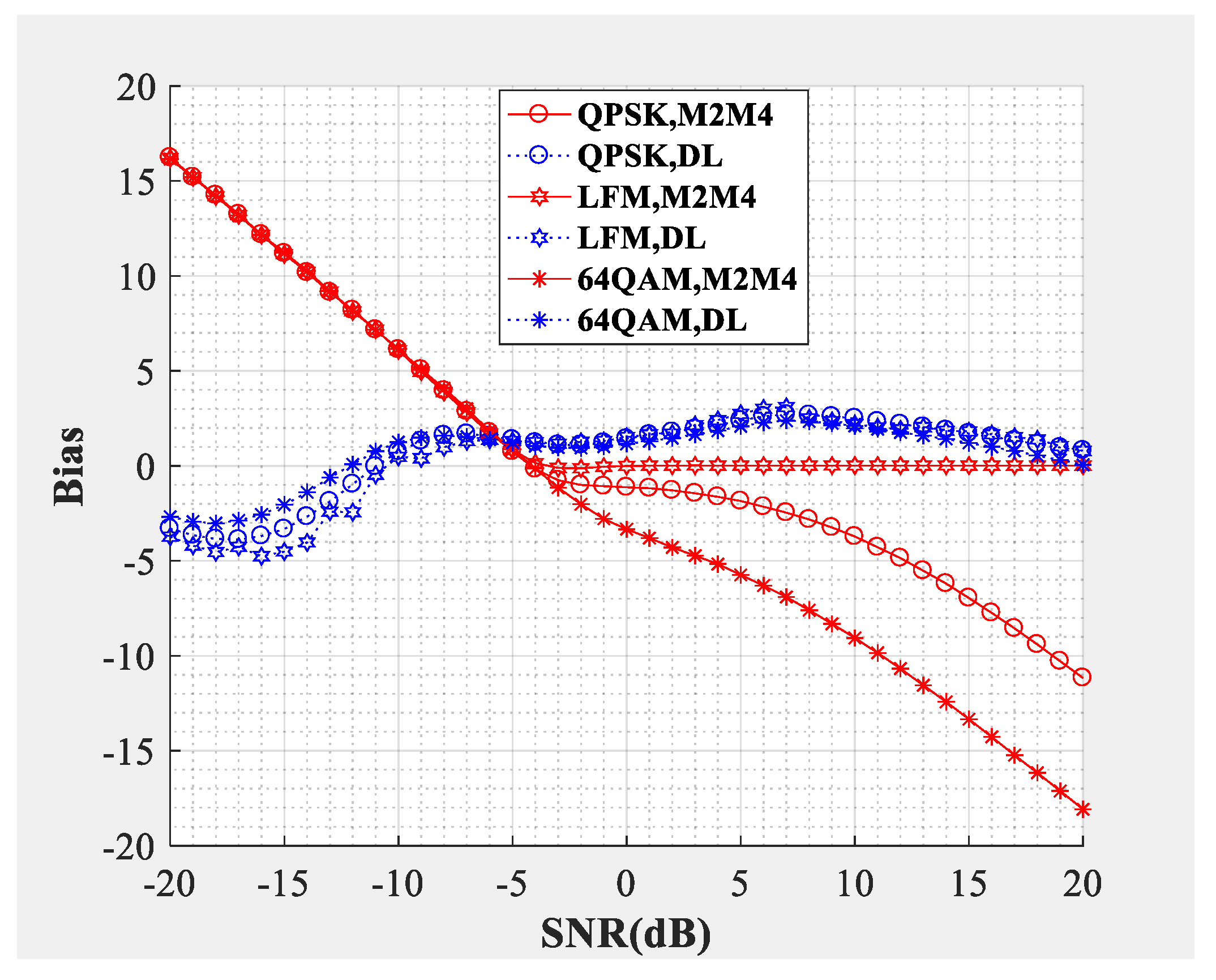
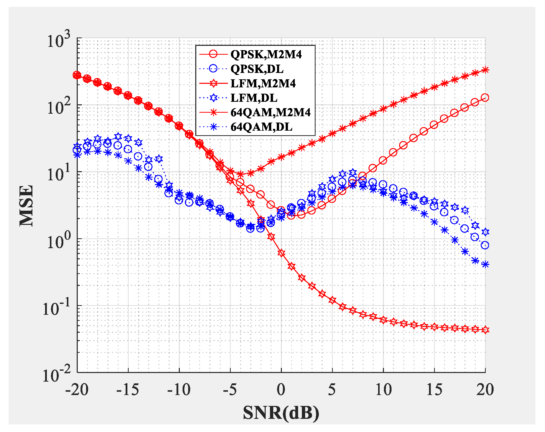
Figure 8 and
Figure 9 compare the SNR estimation performance of DL-based estimator and M2M4 estimator for the intermediate frequency signal. The modulation types used to test were LFM, QPSK and 64QAM IF signals (differentiated by different colors) with a carrier frequency of 10 MHz. The dotted line represents the SNR estimator proposed in this paper, and the solid line represents the M2M4 estimator. From the bias shown in
Figure 8 and the MSE shown in
Figure 9, the following conclusions can be drawn: Firstly, the DL-based estimator can effectively estimate the SNR of LFM (analog modulation), QPSK (constant modulus scheme), and 64QAM (multilevel constellation) IF signals from −10 dB to 20 dB. Secondly, compared with the M2M4 estimator, the DL-based estimator is superior for QPSK and 64QAM signals. For the LFM signal, the performance of the DL-based estimator is worse when the SNR is greater than −6 dB, but is superior when the SNR is smaller than −6 dB.
Table 1 lists the average time cost per sample of the DL-based SNR estimator and the M2M4 SNR estimator. The simulation platform was as follows: CPU Intel i7-6800K, GPU Nvidia 1080Ti, memory 24 GB, and OS Ubuntu 16.04. The M2M4 SNR estimator was implemented with Matlab 2016b, mainly using the CPU, while the DL-based SNR estimator runs on the Python platform, mainly using the GPU. The test data was baseband 64QAM data, incoherent QPSK data and the IF 64QAM data, their length was 1000. Since the training of deep neural networks can be performed offline,
Table 1 only lists the average time cost per sample of the test data set.
The computational complexity of the proposed SNR estimation method is mainly determined by the structure of the employed deep neural network. The computational complexity of the convolutional neural network part is
where
denotes the length of the input of the current convolution layer,
is the channel number of the previous layer (which is same as the convolutional kernel number), i.e., the channel number of the input of the current layer,
is the length of the convolutional kernel, and
is the convolutional kernel number of the current layer, i.e., the channel number of the output. For example, for the first layer of the deep neural network shown in
Figure 3,
,
,
,
. The computational complexity of the forward connected neural network part is
where
denotes the neuron number of previous layer, i.e., the length of the input of the current layer, and
is the neuron number of the current layer. While the computational complexity of the M2M4 SNR estimator is
where
is the length of the received signal.
From Equations (22)–(23), the computational complexity of the M2M4 SNR estimator is significantly less than the DL-based SNR estimator. However, the time cost per sample of the DL-based SNR estimator can be greatly reduced, attributed to the parallel processing. The output of different convolution kernels or neurons of a layer can be implemented parallelly, and the estimation of different received signals can also be processed simultaneously. Additionaly, since the technique of accommodating the varying input length is carefully designed in this paper, the computational complexity of the proposed SNR estimation method grows linearly as the length of the received signal increases.


