A New Quadratic Binary Harris Hawk Optimization for Feature Selection


Abstract
1. Introduction
2. Harris Hawk Optimization
2.1. Exploration Phase
2.2. Exploitation Phase
2.2.1. Soft Besiege
2.2.2. Hard Besiege
2.2.3. Soft Besiege with Progressive Rapid Dives
2.2.4. Hard Besiege with Progressive Rapid Dives
3. The Proposed Binary Harris Hawk Optimization
3.1. Representation of Solutions
3.2. Transformation of Solutions
3.3. Binary Harris Hawk Optimization Algorithm
| Algorithm 1. Binary Harris hawk optimization. |
| Inputs: N and T |
| 1: Initialize the Xi for N hawks |
| 2: for (t = 1 to T) |
| 3: Evaluate the fitness value of the hawks, F(X) |
| 4: Define the best solution as Xr |
| 5: for (i = 1 to N) |
| 6: Compute the E0 and J as shown in (2) and (7), respectively |
| 7: Update the E using (1) |
| // Exploration phase // |
| 8: if (|E| ≥ 1) |
| 9: Update the position of the hawk using (3) |
| 10: Calculate the probability using S-shaped or V-shaped transfer function |
| 11: Update new position of the hawk using (17) or (18) |
| // Exploitation phase // |
| 12: elseif (|E| < 1) |
| // Soft besiege // |
| 13: if (r ≥ 0.5) and (|E| ≥ 0.5) |
| 14: Update the position of the hawk as shown in (5) |
| 15: Calculate the probability using S-shaped or V-shaped transfer function |
| 16: Update new position of the hawk using (17) or (18) |
| // Hard besiege // |
| 17: elseif (r ≥ 0.5) and (|E| < 0.5) |
| 18: Update the position of the hawk using (8) |
| 19: Calculate the probability using S-shaped or V-shaped transfer function |
| 20: Update new position of the hawk using (17) or (18) |
| // Soft besiege with progressive rapid dives // |
| 21: elseif (r < 0.5) and (|E| ≥ 0.5) |
| 22: Update the position of the hawk using (13) |
| 23: Calculate the probability using S-shaped or V-shaped transfer function |
| 24: Update new position of the hawk using (17) or (18) |
| // Hard besiege with progressive rapid dives // |
| 25: elseif (r < 0.5) and (|E| < 0.5) |
| 26: Update the position of the hawk using (16) |
| 27: Calculate the probability using S-shaped or V-shaped transfer function |
| 28: Update new position of the hawk using (17) or (18) |
| 29: end if |
| 30: end if |
| 31: next i |
| 32: Update Xr if there is a better solution |
| 33: next t |
| Output: Global best solution |
4. The Proposed Quadratic Binary Harris Hawk Optimization
| Algorithm 2. Quadratic binary Harris hawk optimization. |
| Inputs: N and T |
| 1: Initialize the Xi for N hawks |
| 2: for (t = 1 to T) |
| 3: Evaluate the fitness value of the hawks, F(X) |
| 4: Define the best solution as Xr |
| 5: for (i = 1 to N) |
| 6: Compute the E0 and J as shown in (2) and (7), respectively |
| 7: Update the E using (1) |
| // Exploration phase // |
| 8: if (|E| ≥ 1) |
| 9: Update the position of the hawk using (3) |
| 10: Calculate the probability using quadratic transfer function |
| 11: Update new position of the hawk using (19) |
| // Exploitation phase // |
| 12: elseif (|E| < 1) |
| // Soft besiege // |
| 13: if (r ≥ 0.5) and (|E| ≥ 0.5) |
| 14: Update the position of the hawk as shown in (5) |
| 15: Calculate the probability using quadratic transfer function |
| 16: Update new position of the hawk using (19) |
| // Hard besiege // |
| 17: elseif (r ≥ 0.5) and (|E| < 0.5) |
| 18: Update the position of the hawk using (8) |
| 19: Calculate the probability using quadratic transfer function |
| 20: Update new position of the hawk using (19) |
| // Soft besiege with progressive rapid dives // |
| 21: elseif (r < 0.5) and (|E| ≥ 0.5) |
| 22: Update the position of the hawk as shown in (13) |
| 23: Calculate the probability using quadratic transfer function |
| 24: Update new position of the hawk using (19) |
| // Hard besiege with progressive rapid dives // |
| 25: elseif (r < 0.5) and (|E| < 0.5) |
| 26: Update the position of the hawk using (16) |
| 27: Calculate the probability using quadratic transfer function |
| 28: Update new position of the hawk using (19) |
| 29: end if |
| 30: end if |
| 31: next i |
| 32: Update Xr if there is a better solution |
| 33: next t |
| Output: Global best solution |
5. Application of Proposed BHHO and QBHHO for Feature Selection
6. Experiment and Results
6.1. Dataset
6.2. Parameter Settings
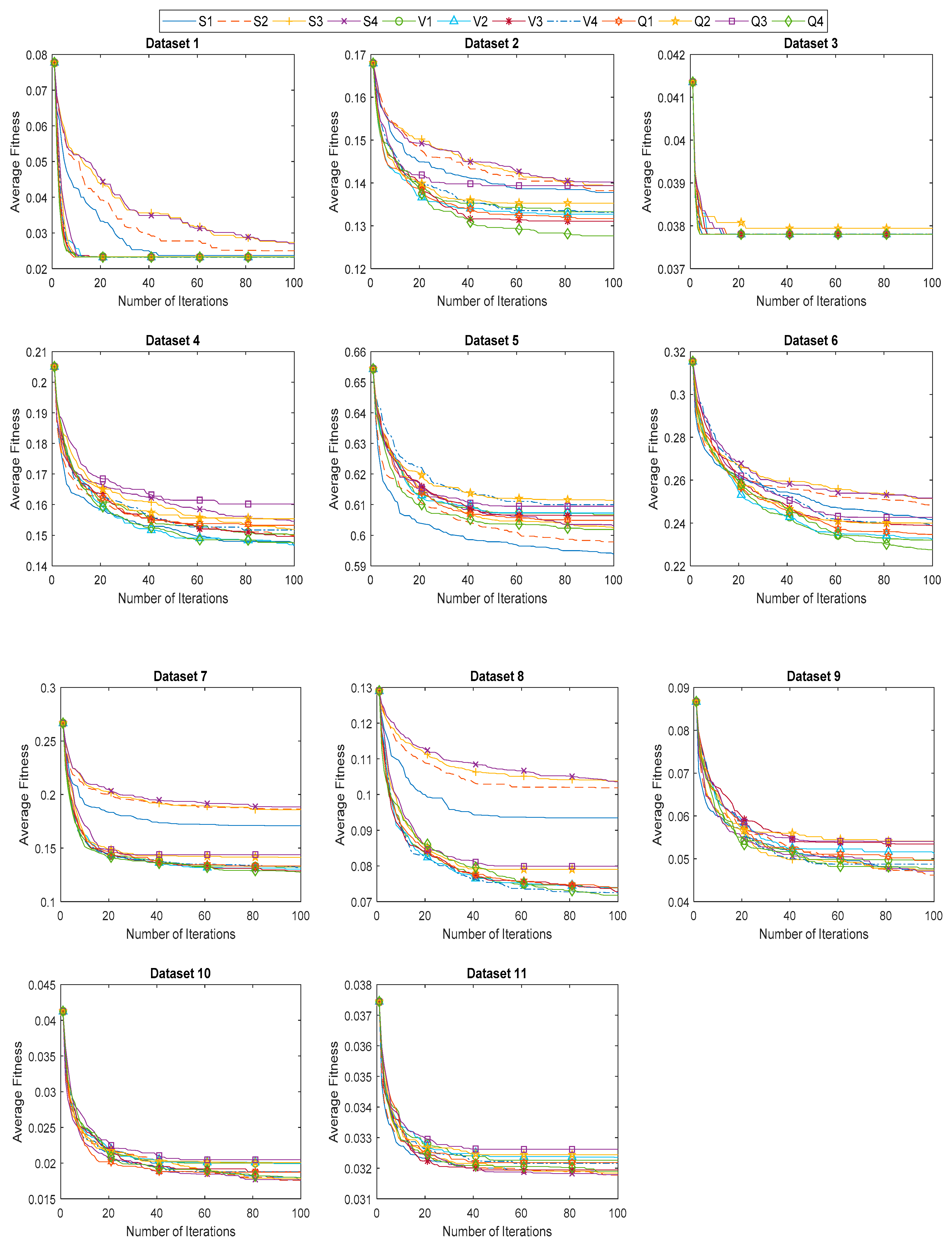
6.3. Evaluation of Proposed BHHO and QBHHO Algorithms
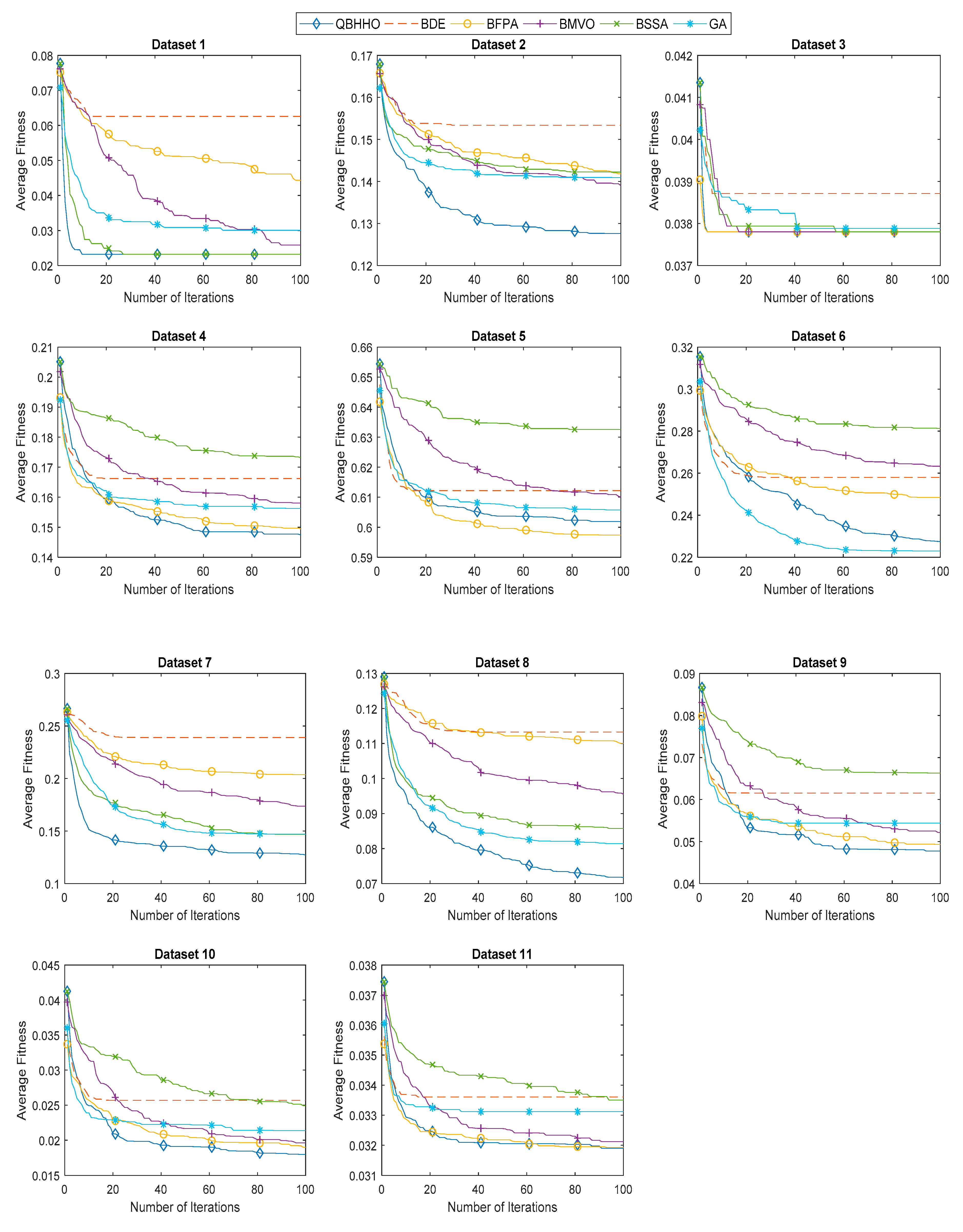
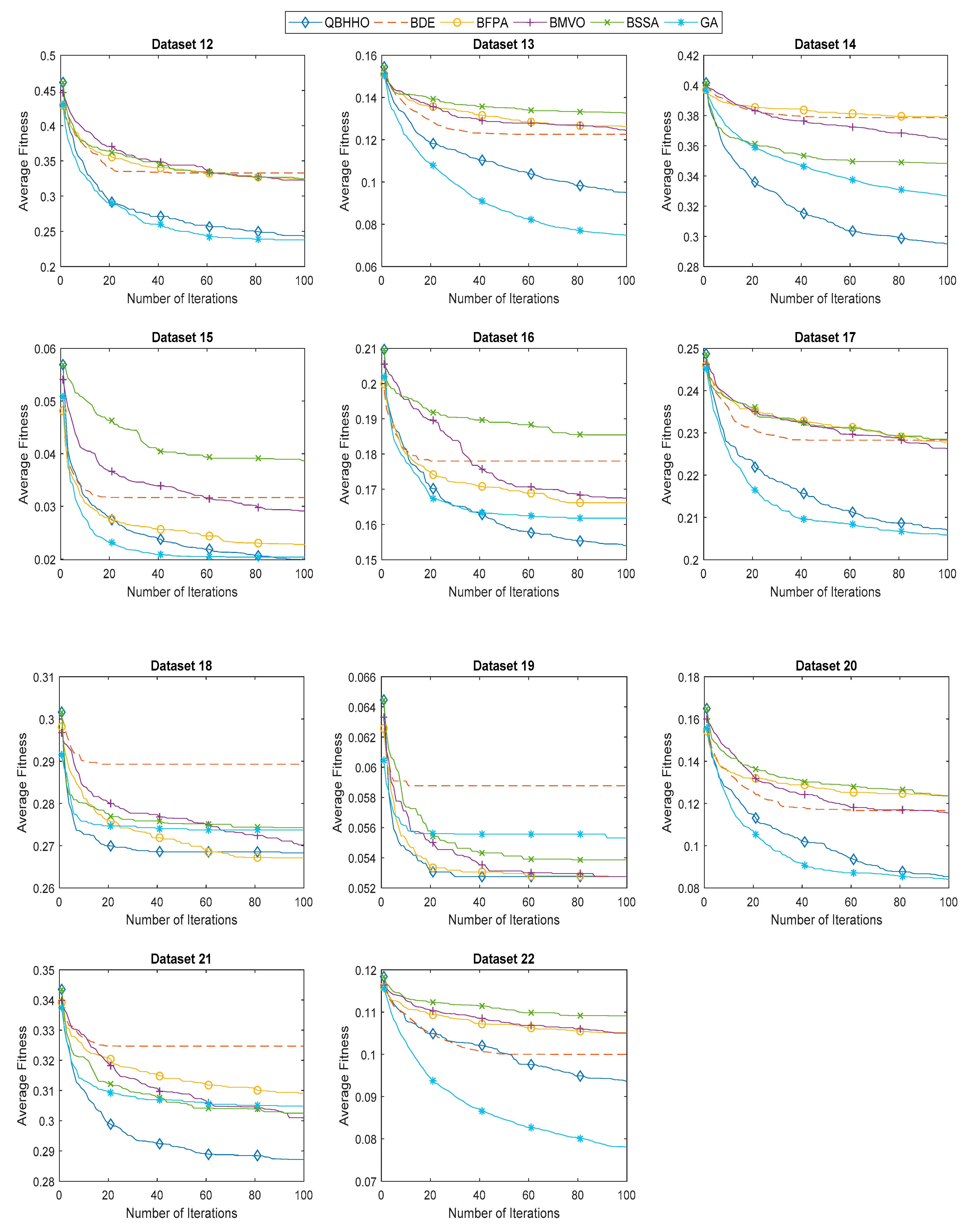
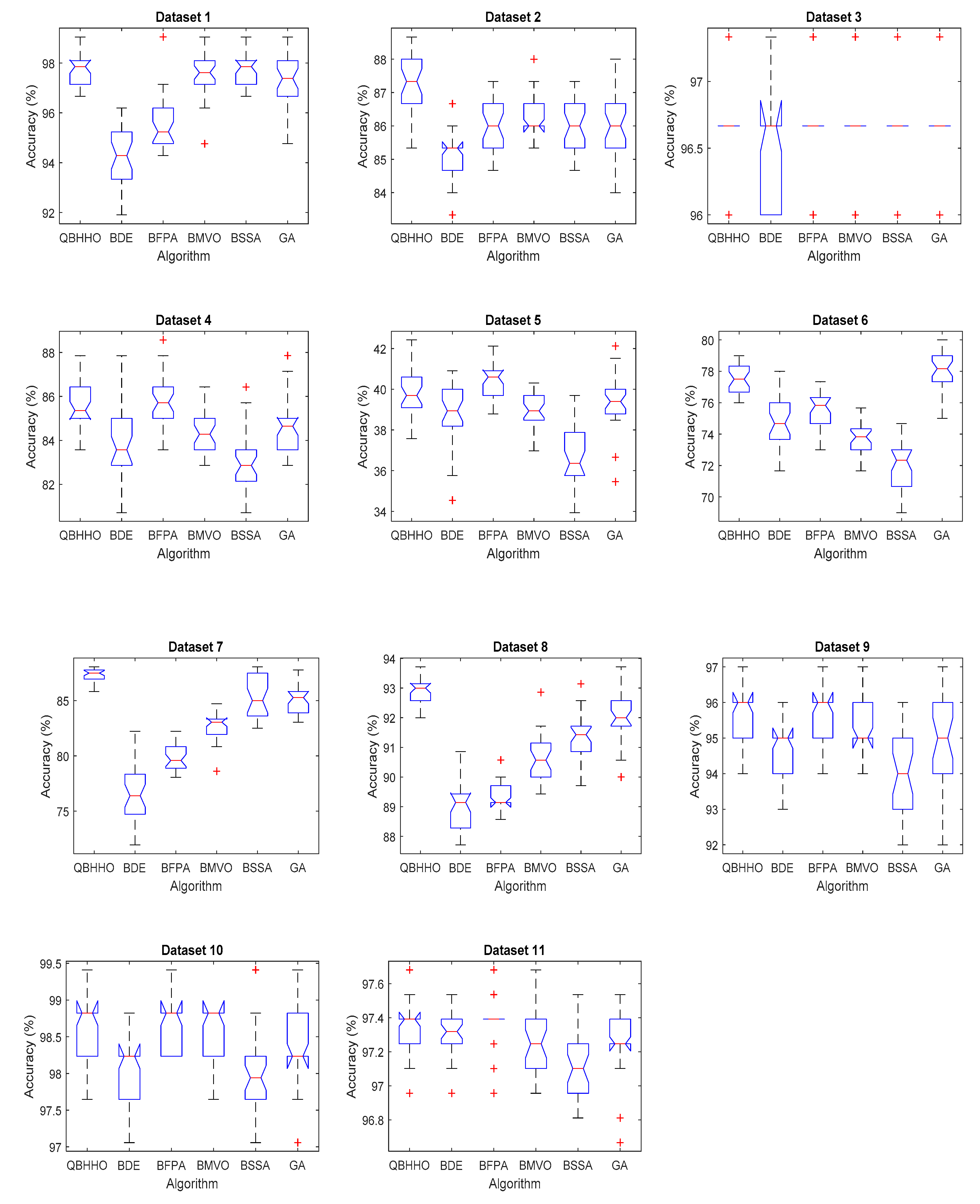
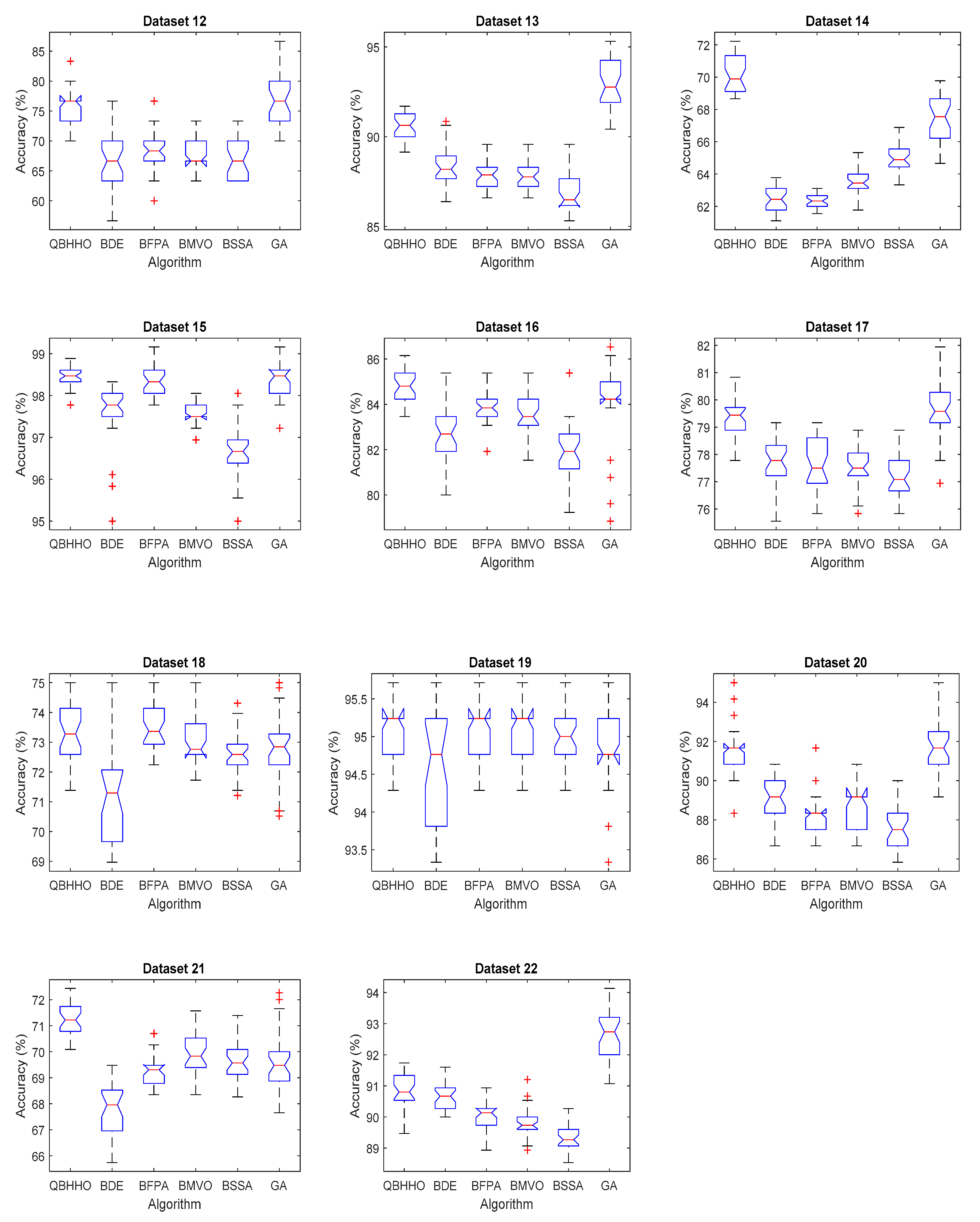
6.4. Comparison with Other Metaheuristic Algorithms
7. Conclusions
Author Contributions
Funding
Acknowledgments
Conflicts of Interest
References
- Tran, B.; Xue, B.; Zhang, M. Genetic programming for multiple-feature construction on high-dimensional classification. Pattern Recognit. 2019, 93, 404–417. [Google Scholar] [CrossRef]
- Qiu, C. A Novel Multi-Swarm Particle Swarm Optimization for Feature Selection. Genet. Program. Evol. Mach. 2019, 1–27. [Google Scholar] [CrossRef]
- Jia, H.; Li, J.; Song, W.; Peng, X.; Lang, C.; Li, Y. Spotted Hyena Optimization Algorithm With Simulated Annealing for Feature Selection. IEEE Access 2019, 7, 71943–71962. [Google Scholar] [CrossRef]
- Hu, L.; Gao, W.; Zhao, K.; Zhang, P.; Wang, F. Feature selection considering two types of feature relevancy and feature interdependency. Expert Syst. Appl. 2018, 93, 423–434. [Google Scholar] [CrossRef]
- Yan, K.; Ma, L.; Dai, Y.; Shen, W.; Ji, Z.; Xie, D. Cost-sensitive and sequential feature selection for chiller fault detection and diagnosis. Int. J. Refrig. 2018, 86, 401–409. [Google Scholar] [CrossRef]
- Bharti, K.K.; Singh, P.K. Opposition chaotic fitness mutation based adaptive inertia weight BPSO for feature selection in text clustering. Appl. Soft Comput. 2016, 43, 20–34. [Google Scholar] [CrossRef]
- Emary, E.; Zawbaa, H.M. Feature selection via Lèvy Antlion optimization. Pattern Anal. Appl. 2018, 22, 857–876. [Google Scholar] [CrossRef]
- Too, J.; Abdullah, A.R.; Saad, N.M. Hybrid Binary Particle Swarm Optimization Differential Evolution-Based Feature Selection for EMG Signals Classification. Axioms 2019, 8, 79. [Google Scholar] [CrossRef]
- Emary, E.; Zawbaa, H.M.; Hassanien, A.E. Binary grey wolf optimization approaches for feature selection. Neurocomputing 2016, 172, 371–381. [Google Scholar] [CrossRef]
- Tu, Q.; Chen, X.; Liu, X. Multi-strategy ensemble grey wolf optimizer and its application to feature selection. Appl. Soft Comput. 2019, 76, 16–30. [Google Scholar] [CrossRef]
- Sindhu, R.; Ngadiran, R.; Yacob, Y.M.; Zahri, N.A.H.; Hariharan, M. Sine–cosine algorithm for feature selection with elitism strategy and new updating mechanism. Neural Comput. Appl. 2017, 28, 2947–2958. [Google Scholar] [CrossRef]
- Hemanth, D.J.; Anitha, J. Modified Genetic Algorithm approaches for classification of abnormal Magnetic Resonance Brain tumour images. Appl. Soft Comput. 2019, 75, 21–28. [Google Scholar] [CrossRef]
- Kumar, V.; Kaur, A. Binary spotted hyena optimizer and its application to feature selection. J. Ambient. Intell. Humaniz. Comput. 2019, 1–21. [Google Scholar] [CrossRef]
- Al-Madi, N.; Faris, H.; Mirjalili, S. Binary multi-verse optimization algorithm for global optimization and discrete problems. Int. J. Mach. Learn. Cybern. 2019, 1–21. [Google Scholar] [CrossRef]
- Sayed, G.I.; Tharwat, A.; Hassanien, A.E. Chaotic dragonfly algorithm: An improved metaheuristic algorithm for feature selection. Appl. Intell. 2019, 49, 188–205. [Google Scholar] [CrossRef]
- Heidari, A.A.; Mirjalili, S.; Faris, H.; Aljarah, I.; Mafarja, M.; Chen, H. Harris hawks optimization: Algorithm and applications. Futur. Gener. Comput. Syst. 2019, 97, 849–872. [Google Scholar] [CrossRef]
- Wolpert, D.; Macready, W. No free lunch theorems for optimization. IEEE Trans. Evol. Comput. 1997, 1, 67–82. [Google Scholar] [CrossRef]
- Mirjalili, S.; Lewis, A. S-shaped versus V-shaped transfer functions for binary Particle Swarm Optimization. Swarm Evol. Comput. 2013, 9, 1–14. [Google Scholar] [CrossRef]
- Saremi, S.; Mirjalili, S.; Lewis, A. How important is a transfer function in discrete heuristic algorithms. Neural Comput. Applic. 2015, 26, 625–640. [Google Scholar] [CrossRef]
- Rodrigues, D.; Pereira, L.A.; Nakamura, R.Y.; Costa, K.A.; Yang, X.-S.; Souza, A.N.; Papa, J.P. A wrapper approach for feature selection based on Bat Algorithm and Optimum-Path Forest. Expert Syst. Appl. 2014, 41, 2250–2258. [Google Scholar] [CrossRef]
- Rashedi, E.; Nezamabadi-pour, H.; Saryazdi, S. BGSA: Binary gravitational search algorithm. Nat Comput 2010, 9, 727–745. [Google Scholar] [CrossRef]
- Jordehi, A.R. Binary particle swarm optimisation with quadratic transfer function: A new binary optimisation algorithm for optimal scheduling of appliances in smart homes. Appl. Soft Comput. 2019, 78, 465–480. [Google Scholar] [CrossRef]
- Hancer, E.; Xue, B.; Karaboga, D.; Zhang, M. A binary ABC algorithm based on advanced similarity scheme for feature selection. Appl. Soft Comput. 2015, 36, 334–348. [Google Scholar] [CrossRef]
- UCI Machine Learning Repository. Available online: https://archive.ics.uci.edu/ml/index.php (accessed on 24 March 2019).
- Xue, B.; Zhang, M.; Browne, W.N. Particle swarm optimisation for feature selection in classification: Novel initialisation and updating mechanisms. Appl. Soft Comput. 2014, 18, 261–276. [Google Scholar] [CrossRef]
- Mafarja, M.; Aljarah, I.; Faris, H.; Hammouri, A.I.; Al-Zoubi, A.M.; Mirjalili, S. Binary grasshopper optimisation algorithm approaches for feature selection problems. Expert Syst. Appl. 2019, 117, 267–286. [Google Scholar] [CrossRef]
- Mafarja, M.; Aljarah, I.; Heidari, A.A.; Faris, H.; Fournier-Viger, P.; Li, X.; Mirjalili, S. Binary dragonfly optimization for feature selection using time-varying transfer functions. Knowl. Based Syst. 2018, 161, 185–204. [Google Scholar] [CrossRef]
- Faris, H.; Mafarja, M.M.; Heidari, A.A.; Aljarah, I.; Al-Zoubi, A.M.; Mirjalili, S.; Fujita, H. An efficient binary Salp Swarm Algorithm with crossover scheme for feature selection problems. Knowl. Based Syst. 2018, 154, 43–67. [Google Scholar] [CrossRef]
- Emary, E.; Zawbaa, H.M.; Hassanien, A.E. Binary ant lion approaches for feature selection. Neurocomputing 2016, 213, 54–65. [Google Scholar] [CrossRef]
- Zawbaa, H.M.; Emary, E.; Grosan, C. Feature Selection via Chaotic Antlion Optimization. PLoS ONE 2016, 11, e0150652. [Google Scholar] [CrossRef]
- Too, J.; Abdullah, A.R.; Saad, N.M. A New Co-Evolution Binary Particle Swarm Optimization with Multiple Inertia Weight Strategy for Feature Selection. Informatics 2019, 6, 21. [Google Scholar] [CrossRef]
- Zorarpacı, E.; Özel, S.A. A hybrid approach of differential evolution and artificial bee colony for feature selection. Expert Syst. Appl. 2016, 62, 91–103. [Google Scholar] [CrossRef]
- Rodrigues, D.; Yang, X.S.; De Souza, A.N.; Papa, J.P. Binary Flower Pollination Algorithm and Its Application to Feature Selection. In Recent Advances in Swarm Intelligence and Evolutionary Computation; Studies in Computational Intelligence; Springer: Cham, Switzerland, 2015; pp. 85–100. ISBN 978-3-319-13825-1. [Google Scholar]
- De Stefano, C.; Fontanella, F.; Marrocco, C.; Di Freca, A.S. A GA-based feature selection approach with an application to handwritten character recognition. Pattern Recognit. Lett. 2014, 35, 130–141. [Google Scholar] [CrossRef]


| S-Shaped Family | Transfer Function | V-Shaped Family | Transfer Function |
|---|---|---|---|
| S1 | V1 | ||
| S2 | V2 | ||
| S3 | V3 | ||
| S4 | V4 |
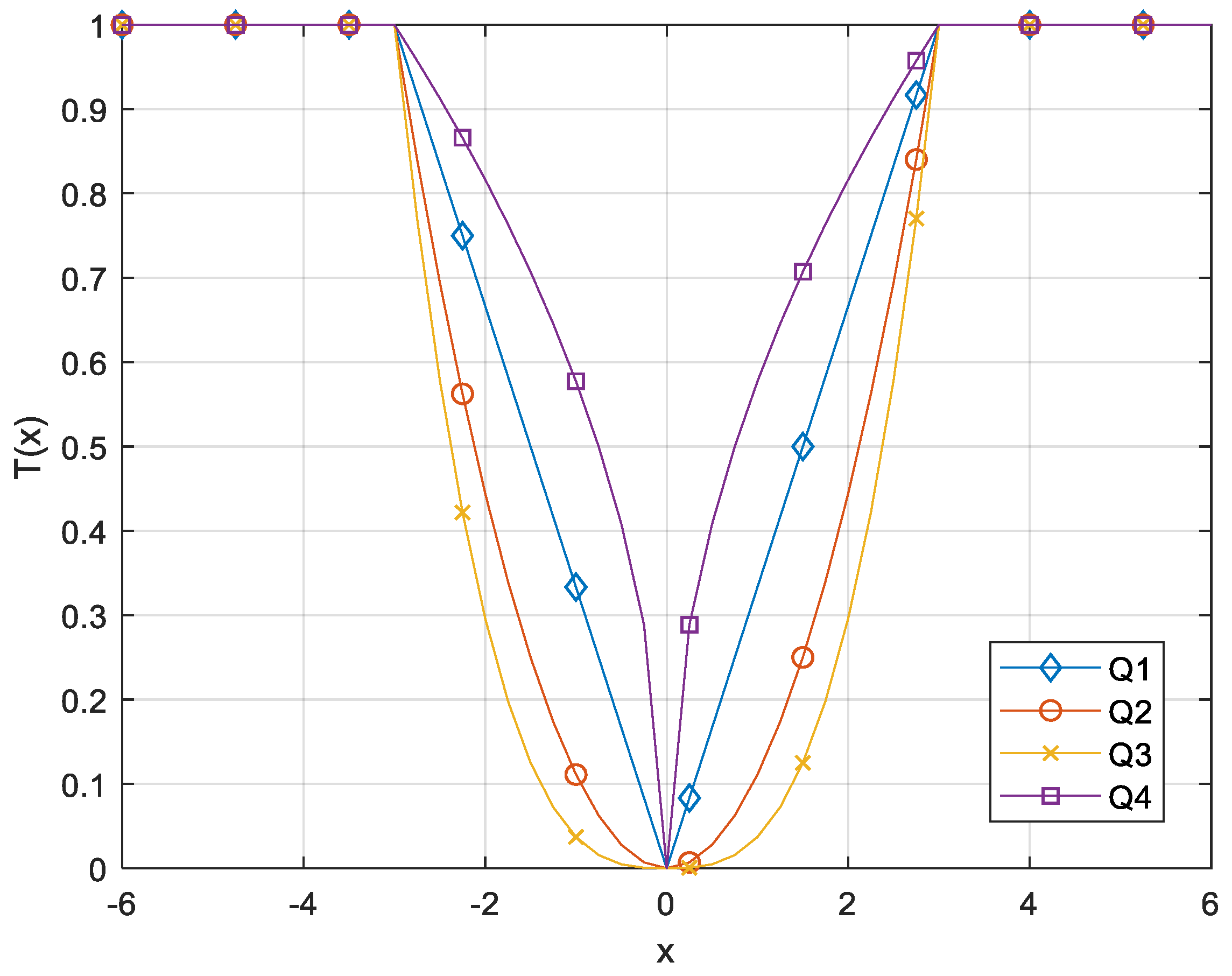
| Name | Transfer Function |
|---|---|
| Q1 | |
| Q2 | |
| Q3 | |
| Q4 |
| No. | Dataset | Number of Instances | Number of Features |
|---|---|---|---|
| 1 | Glass | 214 | 10 |
| 2 | Hepatitis | 155 | 19 |
| 3 | Iris | 150 | 4 |
| 4 | Lymphography | 148 | 18 |
| 5 | Primary Tumor | 339 | 17 |
| 6 | Soybean | 307 | 35 |
| 7 | Horse Colic | 368 | 27 |
| 8 | Ionosphere | 351 | 34 |
| 9 | Zoo | 101 | 16 |
| 10 | Wine | 178 | 13 |
| 11 | Breast Cancer W | 699 | 9 |
| 12 | Lung Cancer | 32 | 56 |
| 13 | Musk 1 | 476 | 166 |
| 14 | Arrhythmia | 452 | 279 |
| 15 | Dermatology | 366 | 34 |
| 16 | SPECT Heart | 267 | 22 |
| 17 | Libras Movement | 360 | 90 |
| 18 | ILPD | 583 | 10 |
| 19 | Seeds | 210 | 7 |
| 20 | LSVT | 126 | 310 |
| 21 | Diabetic | 1151 | 19 |
| 22 | Parkinson | 756 | 754 |
| Dataset | Best Fitness Value | |||||||||||
|---|---|---|---|---|---|---|---|---|---|---|---|---|
| S1 | S2 | S3 | S4 | V1 | V2 | V3 | V4 | Q1 | Q2 | Q3 | Q4 | |
| 1 | 0.0104 | 0.0104 | 0.0104 | 0.0104 | 0.0104 | 0.0104 | 0.0104 | 0.0104 | 0.0104 | 0.0104 | 0.0104 | 0.0104 |
| 2 | 0.1180 | 0.1214 | 0.1209 | 0.1235 | 0.1143 | 0.1204 | 0.1138 | 0.1143 | 0.1143 | 0.1143 | 0.1143 | 0.1143 |
| 3 | 0.0314 | 0.0314 | 0.0314 | 0.0314 | 0.0314 | 0.0314 | 0.0314 | 0.0314 | 0.0314 | 0.0314 | 0.0314 | 0.0314 |
| 4 | 0.1198 | 0.1204 | 0.1291 | 0.1269 | 0.1230 | 0.1230 | 0.1230 | 0.1230 | 0.1198 | 0.1230 | 0.1230 | 0.1230 |
| 5 | 0.5771 | 0.5771 | 0.5771 | 0.5849 | 0.5795 | 0.5771 | 0.5885 | 0.5879 | 0.5885 | 0.5908 | 0.5885 | 0.5765 |
| 6 | 0.2156 | 0.2268 | 0.2341 | 0.2337 | 0.2110 | 0.2077 | 0.2077 | 0.2171 | 0.2171 | 0.2215 | 0.2143 | 0.2116 |
| 7 | 0.1472 | 0.1621 | 0.1463 | 0.1559 | 0.1190 | 0.1190 | 0.1190 | 0.1190 | 0.1190 | 0.1190 | 0.1190 | 0.1190 |
| 8 | 0.0719 | 0.0903 | 0.0954 | 0.0966 | 0.0637 | 0.0637 | 0.0659 | 0.0637 | 0.0659 | 0.0691 | 0.0688 | 0.0637 |
| 9 | 0.0353 | 0.0341 | 0.0335 | 0.0335 | 0.0334 | 0.0334 | 0.0334 | 0.0248 | 0.0334 | 0.0335 | 0.0341 | 0.0334 |
| 10 | 0.0112 | 0.0104 | 0.0112 | 0.0104 | 0.0155 | 0.0104 | 0.0104 | 0.0104 | 0.0104 | 0.0104 | 0.0112 | 0.0104 |
| 11 | 0.0303 | 0.0303 | 0.0303 | 0.0303 | 0.0303 | 0.0303 | 0.0303 | 0.0303 | 0.0303 | 0.0303 | 0.0303 | 0.0303 |
| 12 | 0.2032 | 0.2356 | 0.2342 | 0.2683 | 0.1985 | 0.1670 | 0.1994 | 0.1987 | 0.1989 | 0.1989 | 0.1680 | 0.1670 |
| 13 | 0.1080 | 0.1051 | 0.1080 | 0.1080 | 0.0752 | 0.0761 | 0.0814 | 0.0791 | 0.0822 | 0.0796 | 0.0786 | 0.0843 |
| 14 | 0.3359 | 0.3488 | 0.3562 | 0.3615 | 0.2535 | 0.2555 | 0.2533 | 0.2579 | 0.2600 | 0.2754 | 0.2620 | 0.2754 |
| 15 | 0.0178 | 0.0172 | 0.0172 | 0.0172 | 0.0164 | 0.0142 | 0.0142 | 0.0148 | 0.0142 | 0.0154 | 0.0166 | 0.0148 |
| 16 | 0.1463 | 0.1463 | 0.1492 | 0.1459 | 0.1369 | 0.1412 | 0.1479 | 0.1450 | 0.1445 | 0.1445 | 0.1450 | 0.1412 |
| 17 | 0.2110 | 0.2124 | 0.2142 | 0.2107 | 0.1800 | 0.1806 | 0.1855 | 0.1857 | 0.1884 | 0.1914 | 0.1855 | 0.1925 |
| 18 | 0.2525 | 0.2525 | 0.2542 | 0.2542 | 0.2525 | 0.2525 | 0.2525 | 0.2525 | 0.2525 | 0.2525 | 0.2542 | 0.2525 |
| 19 | 0.0467 | 0.0467 | 0.0467 | 0.0467 | 0.0467 | 0.0467 | 0.0467 | 0.0467 | 0.0467 | 0.0467 | 0.0467 | 0.0467 |
| 20 | 0.0970 | 0.0972 | 0.0960 | 0.1033 | 0.0416 | 0.0510 | 0.0502 | 0.0498 | 0.0595 | 0.0582 | 0.0581 | 0.0505 |
| 21 | 0.2824 | 0.2824 | 0.2895 | 0.2895 | 0.2755 | 0.2793 | 0.2759 | 0.2759 | 0.2759 | 0.2781 | 0.2781 | 0.2755 |
| 22 | 0.0964 | 0.0985 | 0.0977 | 0.0953 | 0.0775 | 0.0745 | 0.0838 | 0.0732 | 0.0756 | 0.0775 | 0.0725 | 0.0843 |
| Dataset | Mean Fitness Value | |||||||||||
|---|---|---|---|---|---|---|---|---|---|---|---|---|
| S1 | S2 | S3 | S4 | V1 | V2 | V3 | V4 | Q1 | Q2 | Q3 | Q4 | |
| 1 | 0.0237 | 0.0250 | 0.0273 | 0.0270 | 0.0232 | 0.0232 | 0.0232 | 0.0232 | 0.0232 | 0.0233 | 0.0232 | 0.0232 |
| 2 | 0.1378 | 0.1382 | 0.1394 | 0.1402 | 0.1332 | 0.1327 | 0.1311 | 0.1331 | 0.1317 | 0.1353 | 0.1394 | 0.1276 |
| 3 | 0.0378 | 0.0378 | 0.0378 | 0.0378 | 0.0378 | 0.0378 | 0.0378 | 0.0378 | 0.0378 | 0.0379 | 0.0378 | 0.0378 |
| 4 | 0.1464 | 0.1500 | 0.1519 | 0.1546 | 0.1502 | 0.1469 | 0.1496 | 0.1513 | 0.1533 | 0.1554 | 0.1602 | 0.1474 |
| 5 | 0.5938 | 0.5978 | 0.6023 | 0.6030 | 0.6067 | 0.6073 | 0.6064 | 0.6100 | 0.6049 | 0.6114 | 0.6095 | 0.6019 |
| 6 | 0.2416 | 0.2484 | 0.2515 | 0.2516 | 0.2320 | 0.2323 | 0.2387 | 0.2393 | 0.2347 | 0.2400 | 0.2426 | 0.2275 |
| 7 | 0.1709 | 0.1865 | 0.1858 | 0.1885 | 0.1323 | 0.1304 | 0.1286 | 0.1320 | 0.1332 | 0.1412 | 0.1438 | 0.1272 |
| 8 | 0.0935 | 0.1019 | 0.1038 | 0.1036 | 0.0739 | 0.0740 | 0.0728 | 0.0725 | 0.0739 | 0.0790 | 0.0799 | 0.0717 |
| 9 | 0.0474 | 0.0462 | 0.0473 | 0.0471 | 0.0497 | 0.0513 | 0.0535 | 0.0484 | 0.0496 | 0.0541 | 0.0541 | 0.0477 |
| 10 | 0.0175 | 0.0176 | 0.0178 | 0.0177 | 0.0200 | 0.0199 | 0.0188 | 0.0188 | 0.0187 | 0.0201 | 0.0205 | 0.0180 |
| 11 | 0.0319 | 0.0318 | 0.0318 | 0.0318 | 0.0323 | 0.0324 | 0.0319 | 0.0322 | 0.0322 | 0.0324 | 0.0326 | 0.0319 |
| 12 | 0.3180 | 0.3089 | 0.3109 | 0.3214 | 0.2561 | 0.2530 | 0.2517 | 0.2538 | 0.2551 | 0.2617 | 0.2532 | 0.2431 |
| 13 | 0.1214 | 0.1215 | 0.1256 | 0.1248 | 0.1005 | 0.0997 | 0.1011 | 0.1043 | 0.1037 | 0.0983 | 0.0986 | 0.0951 |
| 14 | 0.3590 | 0.3686 | 0.3714 | 0.3739 | 0.2814 | 0.2835 | 0.2798 | 0.2821 | 0.2853 | 0.3020 | 0.3007 | 0.2950 |
| 15 | 0.0216 | 0.0223 | 0.0242 | 0.0251 | 0.0206 | 0.0221 | 0.0215 | 0.0236 | 0.0211 | 0.0234 | 0.0221 | 0.0199 |
| 16 | 0.1643 | 0.1633 | 0.1651 | 0.1657 | 0.1632 | 0.1603 | 0.1635 | 0.1667 | 0.1712 | 0.1723 | 0.1692 | 0.1540 |
| 17 | 0.2256 | 0.2272 | 0.2263 | 0.2276 | 0.2036 | 0.2054 | 0.2065 | 0.2100 | 0.2054 | 0.2094 | 0.2043 | 0.2069 |
| 18 | 0.2677 | 0.2671 | 0.2675 | 0.2678 | 0.2679 | 0.2698 | 0.2705 | 0.2693 | 0.2706 | 0.2733 | 0.2739 | 0.2683 |
| 19 | 0.0527 | 0.0527 | 0.0527 | 0.0527 | 0.0530 | 0.0529 | 0.0527 | 0.0527 | 0.0529 | 0.0531 | 0.0539 | 0.0527 |
| 20 | 0.1193 | 0.1200 | 0.1190 | 0.1202 | 0.0806 | 0.0779 | 0.0811 | 0.0790 | 0.0830 | 0.0845 | 0.0860 | 0.0854 |
| 21 | 0.3007 | 0.3030 | 0.3051 | 0.3055 | 0.2908 | 0.2909 | 0.2901 | 0.2893 | 0.2892 | 0.2946 | 0.2964 | 0.2873 |
| 22 | 0.1037 | 0.1042 | 0.1044 | 0.1039 | 0.0921 | 0.0903 | 0.0943 | 0.0944 | 0.0907 | 0.0916 | 0.0915 | 0.0936 |
| Dataset | Standard Deviation of Fitness Value | |||||||||||
|---|---|---|---|---|---|---|---|---|---|---|---|---|
| S1 | S2 | S3 | S4 | V1 | V2 | V3 | V4 | Q1 | Q2 | Q3 | Q4 | |
| 1 | 0.0075 | 0.0091 | 0.0098 | 0.0095 | 0.0070 | 0.0070 | 0.0070 | 0.0070 | 0.0070 | 0.0071 | 0.0070 | 0.0070 |
| 2 | 0.0070 | 0.0078 | 0.0080 | 0.0065 | 0.0108 | 0.0076 | 0.0087 | 0.0087 | 0.0105 | 0.0106 | 0.0108 | 0.0085 |
| 3 | 0.0033 | 0.0033 | 0.0033 | 0.0033 | 0.0033 | 0.0033 | 0.0033 | 0.0033 | 0.0033 | 0.0034 | 0.0033 | 0.0033 |
| 4 | 0.0117 | 0.0110 | 0.0109 | 0.0113 | 0.0139 | 0.0112 | 0.0112 | 0.0133 | 0.0133 | 0.0183 | 0.0198 | 0.0115 |
| 5 | 0.0073 | 0.0087 | 0.0077 | 0.0076 | 0.0093 | 0.0114 | 0.0081 | 0.0094 | 0.0086 | 0.0114 | 0.0126 | 0.0098 |
| 6 | 0.0121 | 0.0096 | 0.0090 | 0.0110 | 0.0131 | 0.0120 | 0.0126 | 0.0127 | 0.0118 | 0.0140 | 0.0183 | 0.0103 |
| 7 | 0.0133 | 0.0119 | 0.0115 | 0.0109 | 0.0117 | 0.0122 | 0.0100 | 0.0105 | 0.0104 | 0.0179 | 0.0180 | 0.0066 |
| 8 | 0.0068 | 0.0054 | 0.0048 | 0.0045 | 0.0054 | 0.0059 | 0.0047 | 0.0046 | 0.0052 | 0.0042 | 0.0088 | 0.0040 |
| 9 | 0.0064 | 0.0078 | 0.0084 | 0.0078 | 0.0123 | 0.0096 | 0.0096 | 0.0107 | 0.0103 | 0.0123 | 0.0102 | 0.0091 |
| 10 | 0.0032 | 0.0030 | 0.0030 | 0.0035 | 0.0034 | 0.0042 | 0.0037 | 0.0042 | 0.0043 | 0.0046 | 0.0048 | 0.0042 |
| 11 | 0.0008 | 0.0009 | 0.0010 | 0.0009 | 0.0012 | 0.0011 | 0.0009 | 0.0010 | 0.0009 | 0.0014 | 0.0014 | 0.0009 |
| 12 | 0.0393 | 0.0354 | 0.0350 | 0.0294 | 0.0375 | 0.0401 | 0.0328 | 0.0359 | 0.0415 | 0.0443 | 0.0389 | 0.0314 |
| 13 | 0.0059 | 0.0062 | 0.0070 | 0.0080 | 0.0091 | 0.0125 | 0.0115 | 0.0104 | 0.0080 | 0.0104 | 0.0125 | 0.0077 |
| 14 | 0.0094 | 0.0081 | 0.0058 | 0.0061 | 0.0183 | 0.0172 | 0.0184 | 0.0146 | 0.0143 | 0.0149 | 0.0169 | 0.0128 |
| 15 | 0.0022 | 0.0025 | 0.0028 | 0.0028 | 0.0027 | 0.0043 | 0.0035 | 0.0048 | 0.0042 | 0.0044 | 0.0039 | 0.0029 |
| 16 | 0.0073 | 0.0077 | 0.0071 | 0.0071 | 0.0187 | 0.0119 | 0.0137 | 0.0173 | 0.0205 | 0.0199 | 0.0198 | 0.0076 |
| 17 | 0.0070 | 0.0069 | 0.0081 | 0.0081 | 0.0107 | 0.0107 | 0.0113 | 0.0096 | 0.0093 | 0.0076 | 0.0122 | 0.0079 |
| 18 | 0.0077 | 0.0070 | 0.0062 | 0.0064 | 0.0072 | 0.0083 | 0.0078 | 0.0073 | 0.0079 | 0.0089 | 0.0085 | 0.0080 |
| 19 | 0.0030 | 0.0030 | 0.0030 | 0.0030 | 0.0030 | 0.0030 | 0.0030 | 0.0030 | 0.0030 | 0.0028 | 0.0037 | 0.0030 |
| 20 | 0.0120 | 0.0118 | 0.0091 | 0.0103 | 0.0155 | 0.0131 | 0.0137 | 0.0132 | 0.0157 | 0.0111 | 0.0112 | 0.0143 |
| 21 | 0.0084 | 0.0079 | 0.0071 | 0.0068 | 0.0076 | 0.0060 | 0.0062 | 0.0067 | 0.0074 | 0.0102 | 0.0094 | 0.0065 |
| 22 | 0.0036 | 0.0030 | 0.0039 | 0.0045 | 0.0079 | 0.0063 | 0.0067 | 0.0083 | 0.0066 | 0.0062 | 0.0081 | 0.0054 |
| Dataset | Average Classification Accuracy | |||||||||||
|---|---|---|---|---|---|---|---|---|---|---|---|---|
| S1 | S2 | S3 | S4 | V1 | V2 | V3 | V4 | Q1 | Q2 | Q3 | Q4 | |
| 1 | 0.9771 | 0.9759 | 0.9737 | 0.9740 | 0.9776 | 0.9776 | 0.9776 | 0.9776 | 0.9776 | 0.9775 | 0.9776 | 0.9776 |
| 2 | 0.8647 | 0.8642 | 0.8633 | 0.8622 | 0.8676 | 0.8680 | 0.8700 | 0.8676 | 0.8691 | 0.8653 | 0.8609 | 0.8736 |
| 3 | 0.9664 | 0.9664 | 0.9664 | 0.9664 | 0.9664 | 0.9664 | 0.9664 | 0.9664 | 0.9664 | 0.9662 | 0.9664 | 0.9664 |
| 4 | 0.8588 | 0.8550 | 0.8529 | 0.8500 | 0.8519 | 0.8548 | 0.8524 | 0.8505 | 0.8488 | 0.8467 | 0.8417 | 0.8545 |
| 5 | 0.4074 | 0.4032 | 0.3986 | 0.3975 | 0.3923 | 0.3918 | 0.3927 | 0.3888 | 0.3944 | 0.3878 | 0.3901 | 0.3978 |
| 6 | 0.7631 | 0.7556 | 0.7516 | 0.7513 | 0.7692 | 0.7687 | 0.7622 | 0.7613 | 0.7668 | 0.7616 | 0.7584 | 0.7742 |
| 7 | 0.8297 | 0.8146 | 0.8157 | 0.8132 | 0.8671 | 0.8691 | 0.8709 | 0.8675 | 0.8662 | 0.8581 | 0.8555 | 0.8723 |
| 8 | 0.9082 | 0.9004 | 0.8990 | 0.8992 | 0.9265 | 0.9263 | 0.9275 | 0.9279 | 0.9264 | 0.9213 | 0.9205 | 0.9289 |
| 9 | 0.9580 | 0.9590 | 0.9573 | 0.9577 | 0.9543 | 0.9527 | 0.9503 | 0.9557 | 0.9543 | 0.9497 | 0.9500 | 0.9563 |
| 10 | 0.9880 | 0.9878 | 0.9876 | 0.9873 | 0.9845 | 0.9843 | 0.9855 | 0.9855 | 0.9857 | 0.9841 | 0.9841 | 0.9867 |
| 11 | 0.9736 | 0.9735 | 0.9735 | 0.9736 | 0.9723 | 0.9726 | 0.9732 | 0.9729 | 0.9727 | 0.9723 | 0.9720 | 0.9732 |
| 12 | 0.6833 | 0.6933 | 0.6911 | 0.6800 | 0.7422 | 0.7456 | 0.7467 | 0.7444 | 0.7433 | 0.7367 | 0.7456 | 0.7556 |
| 13 | 0.8833 | 0.8830 | 0.8786 | 0.8791 | 0.9004 | 0.9014 | 0.8998 | 0.8962 | 0.8972 | 0.9030 | 0.9025 | 0.9065 |
| 14 | 0.6401 | 0.6317 | 0.6299 | 0.6274 | 0.7162 | 0.7141 | 0.7177 | 0.7155 | 0.7122 | 0.6953 | 0.6965 | 0.7027 |
| 15 | 0.9853 | 0.9841 | 0.9816 | 0.9807 | 0.9831 | 0.9818 | 0.9821 | 0.9801 | 0.9829 | 0.9806 | 0.9820 | 0.9842 |
| 16 | 0.8401 | 0.8408 | 0.8385 | 0.8379 | 0.8382 | 0.8415 | 0.8382 | 0.8347 | 0.8301 | 0.8288 | 0.8322 | 0.8481 |
| 17 | 0.7775 | 0.7756 | 0.7767 | 0.7754 | 0.7959 | 0.7944 | 0.7931 | 0.7896 | 0.7943 | 0.7902 | 0.7954 | 0.7931 |
| 18 | 0.7339 | 0.7347 | 0.7342 | 0.7339 | 0.7330 | 0.7307 | 0.7301 | 0.7316 | 0.7300 | 0.7270 | 0.7263 | 0.7327 |
| 19 | 0.9510 | 0.9510 | 0.9510 | 0.9510 | 0.9506 | 0.9508 | 0.9510 | 0.9510 | 0.9508 | 0.9505 | 0.9495 | 0.9510 |
| 20 | 0.8853 | 0.8844 | 0.8853 | 0.8839 | 0.9194 | 0.9222 | 0.9189 | 0.9208 | 0.9169 | 0.9158 | 0.9142 | 0.9153 |
| 21 | 0.6998 | 0.6977 | 0.6956 | 0.6952 | 0.7090 | 0.7087 | 0.7096 | 0.7100 | 0.7104 | 0.7046 | 0.7027 | 0.7126 |
| 22 | 0.9018 | 0.9008 | 0.9003 | 0.9004 | 0.9089 | 0.9103 | 0.9067 | 0.9066 | 0.9104 | 0.9098 | 0.9095 | 0.9083 |
| Dataset | Average Number of Selected Features | |||||||||||
|---|---|---|---|---|---|---|---|---|---|---|---|---|
| S1 | S2 | S3 | S4 | V1 | V2 | V3 | V4 | Q1 | Q2 | Q3 | Q4 | |
| 1 | 1.03 | 1.13 | 1.23 | 1.23 | 1.07 | 1.07 | 1.07 | 1.07 | 1.07 | 1.03 | 1.07 | 1.07 |
| 2 | 7.17 | 7.17 | 7.83 | 7.20 | 4.03 | 3.83 | 4.53 | 3.83 | 4.00 | 3.73 | 3.17 | 4.63 |
| 3 | 1.83 | 1.83 | 1.83 | 1.83 | 1.83 | 1.83 | 1.83 | 1.83 | 1.83 | 1.80 | 1.83 | 1.83 |
| 4 | 12.00 | 11.53 | 11.23 | 10.90 | 6.50 | 5.57 | 6.23 | 5.87 | 6.47 | 6.43 | 6.20 | 6.17 |
| 5 | 12.07 | 11.97 | 11.77 | 11.13 | 8.70 | 8.80 | 8.77 | 8.27 | 9.13 | 9.00 | 9.63 | 9.67 |
| 6 | 24.90 | 22.37 | 19.43 | 18.97 | 12.43 | 11.63 | 11.70 | 10.43 | 13.20 | 13.77 | 12.27 | 14.07 |
| 7 | 6.37 | 8.13 | 9.27 | 9.63 | 2.07 | 2.03 | 2.10 | 2.10 | 2.07 | 1.93 | 2.00 | 2.07 |
| 8 | 8.80 | 11.10 | 12.77 | 12.93 | 3.63 | 3.47 | 3.73 | 3.87 | 3.60 | 3.93 | 3.93 | 4.43 |
| 9 | 9.37 | 8.97 | 8.17 | 8.27 | 7.23 | 7.07 | 6.87 | 7.20 | 7.00 | 6.83 | 7.33 | 7.20 |
| 10 | 7.37 | 7.20 | 7.27 | 6.57 | 6.03 | 5.70 | 5.77 | 5.73 | 5.90 | 5.67 | 6.17 | 6.23 |
| 11 | 5.17 | 4.97 | 5.07 | 5.07 | 4.37 | 4.67 | 4.90 | 4.80 | 4.60 | 4.53 | 4.43 | 4.87 |
| 12 | 25.43 | 29.40 | 28.83 | 25.90 | 5.03 | 6.13 | 4.77 | 4.53 | 5.50 | 5.67 | 7.07 | 6.27 |
| 13 | 96.40 | 94.70 | 89.87 | 85.63 | 30.93 | 34.30 | 30.73 | 25.97 | 32.23 | 38.37 | 34.60 | 40.60 |
| 14 | 73.23 | 110.50 | 137.83 | 139.57 | 13.23 | 11.93 | 10.47 | 11.20 | 9.97 | 8.67 | 8.10 | 18.60 |
| 15 | 24.03 | 22.33 | 20.37 | 20.53 | 13.47 | 13.77 | 12.87 | 13.07 | 13.93 | 14.43 | 14.60 | 14.27 |
| 16 | 13.30 | 12.50 | 11.47 | 11.70 | 6.67 | 7.53 | 7.27 | 6.80 | 6.73 | 6.33 | 6.73 | 7.93 |
| 17 | 47.93 | 45.23 | 47.03 | 46.83 | 13.77 | 16.23 | 15.00 | 15.57 | 15.63 | 14.90 | 15.53 | 19.40 |
| 18 | 4.30 | 4.50 | 4.37 | 4.37 | 3.53 | 3.27 | 3.23 | 3.50 | 3.30 | 3.00 | 2.90 | 3.70 |
| 19 | 2.93 | 2.93 | 2.93 | 2.93 | 2.87 | 2.90 | 2.93 | 2.93 | 2.90 | 2.87 | 2.77 | 2.93 |
| 20 | 176.60 | 174.67 | 167.60 | 162.13 | 27.10 | 28.87 | 25.27 | 20.17 | 25.37 | 35.47 | 30.50 | 46.67 |
| 21 | 6.77 | 7.03 | 7.13 | 7.03 | 5.03 | 4.80 | 4.80 | 4.30 | 4.70 | 4.20 | 3.93 | 5.30 |
| 22 | 487.00 | 454.47 | 425.70 | 404.87 | 144.53 | 115.10 | 144.20 | 141.67 | 145.67 | 172.83 | 144.47 | 210.00 |
| Algorithm | Parameter | Value |
|---|---|---|
| BDE | Number of vectors, N | 10 |
| Maximum number of generations, T | 100 | |
| Crossover rate, CR | 0.9 | |
| BFPA | Number of flowers, N | 10 |
| Maximum number of iterations, T | 100 | |
| Switch probability, P | 0.8 | |
| BSSA | Number of salps, N | 10 |
| Maximum number of iterations, T | 100 | |
| BMVO | Number of universes, N | 10 |
| Maximum number of iterations, T | 100 | |
| Coefficient, WEP | [0.02, 1] | |
| GA | Number of chromosomes, N | 10 |
| Maximum number of generations, T | 100 | |
| Crossover rate, CR | 0.8 | |
| Mutation rate, MR | 0.01 |
| Dataset | Best Fitness Value | |||||
|---|---|---|---|---|---|---|
| QBHHO | BDE | BFPA | BMVO | BSSA | GA | |
| 1 | 0.0104 | 0.0397 | 0.0104 | 0.0104 | 0.0104 | 0.0104 |
| 2 | 0.1143 | 0.1367 | 0.1301 | 0.1220 | 0.1265 | 0.1220 |
| 3 | 0.0314 | 0.0314 | 0.0314 | 0.0314 | 0.0314 | 0.0314 |
| 4 | 0.1230 | 0.1274 | 0.1215 | 0.1371 | 0.1377 | 0.1258 |
| 5 | 0.5765 | 0.5921 | 0.5801 | 0.5963 | 0.6035 | 0.5795 |
| 6 | 0.2116 | 0.2252 | 0.2324 | 0.2455 | 0.2568 | 0.2037 |
| 7 | 0.1190 | 0.1804 | 0.1801 | 0.1538 | 0.1190 | 0.1217 |
| 8 | 0.0637 | 0.0946 | 0.0975 | 0.0722 | 0.0694 | 0.0643 |
| 9 | 0.0334 | 0.0459 | 0.0353 | 0.0341 | 0.0433 | 0.0341 |
| 10 | 0.0104 | 0.0170 | 0.0104 | 0.0163 | 0.0104 | 0.0112 |
| 11 | 0.0303 | 0.0311 | 0.0303 | 0.0306 | 0.0303 | 0.0314 |
| 12 | 0.1670 | 0.2356 | 0.2381 | 0.2679 | 0.2654 | 0.1354 |
| 13 | 0.0843 | 0.0968 | 0.1080 | 0.1080 | 0.1077 | 0.0504 |
| 14 | 0.2754 | 0.3644 | 0.3711 | 0.3447 | 0.3291 | 0.3038 |
| 15 | 0.0148 | 0.0221 | 0.0150 | 0.0237 | 0.0237 | 0.0121 |
| 16 | 0.1412 | 0.1506 | 0.1506 | 0.1506 | 0.1506 | 0.1374 |
| 17 | 0.1925 | 0.2116 | 0.2121 | 0.2137 | 0.2113 | 0.1832 |
| 18 | 0.2525 | 0.2542 | 0.2525 | 0.2525 | 0.2573 | 0.2542 |
| 19 | 0.0467 | 0.0467 | 0.0467 | 0.0467 | 0.0467 | 0.0467 |
| 20 | 0.0505 | 0.0985 | 0.0887 | 0.0946 | 0.0993 | 0.0528 |
| 21 | 0.2755 | 0.3080 | 0.2927 | 0.2852 | 0.2848 | 0.2778 |
| 22 | 0.0843 | 0.0906 | 0.0960 | 0.0913 | 0.1006 | 0.0629 |
| Dataset | Mean Fitness Value | |||||
|---|---|---|---|---|---|---|
| QBHHO | BDE | BFPA | BMVO | BSSA | GA | |
| 1 | 0.0232 | 0.0626 | 0.0444 | 0.0259 | 0.0232 | 0.0301 |
| 2 | 0.1276 | 0.1534 | 0.1418 | 0.1390 | 0.1422 | 0.1409 |
| 3 | 0.0378 | 0.0387 | 0.0378 | 0.0378 | 0.0378 | 0.0379 |
| 4 | 0.1474 | 0.1662 | 0.1495 | 0.1580 | 0.1732 | 0.1563 |
| 5 | 0.6019 | 0.6122 | 0.5974 | 0.6101 | 0.6325 | 0.6058 |
| 6 | 0.2275 | 0.2580 | 0.2485 | 0.2633 | 0.2813 | 0.2230 |
| 7 | 0.1272 | 0.2390 | 0.2036 | 0.1736 | 0.1468 | 0.1469 |
| 8 | 0.0717 | 0.1133 | 0.1100 | 0.0955 | 0.0857 | 0.0814 |
| 9 | 0.0477 | 0.0615 | 0.0494 | 0.0522 | 0.0663 | 0.0544 |
| 10 | 0.0180 | 0.0257 | 0.0190 | 0.0196 | 0.0249 | 0.0214 |
| 11 | 0.0319 | 0.0336 | 0.0319 | 0.0321 | 0.0335 | 0.0331 |
| 12 | 0.2431 | 0.3328 | 0.3236 | 0.3228 | 0.3245 | 0.2377 |
| 13 | 0.0951 | 0.1226 | 0.1261 | 0.1243 | 0.1326 | 0.0746 |
| 14 | 0.2950 | 0.3786 | 0.3788 | 0.3641 | 0.3483 | 0.3269 |
| 15 | 0.0199 | 0.0317 | 0.0228 | 0.0291 | 0.0387 | 0.0204 |
| 16 | 0.1540 | 0.1780 | 0.1662 | 0.1675 | 0.1854 | 0.1618 |
| 17 | 0.2069 | 0.2283 | 0.2278 | 0.2262 | 0.2285 | 0.2059 |
| 18 | 0.2683 | 0.2893 | 0.2671 | 0.2702 | 0.2743 | 0.2737 |
| 19 | 0.0527 | 0.0588 | 0.0527 | 0.0527 | 0.0539 | 0.0553 |
| 20 | 0.0854 | 0.1166 | 0.1236 | 0.1155 | 0.1236 | 0.0839 |
| 21 | 0.2873 | 0.3247 | 0.3088 | 0.3010 | 0.3025 | 0.3048 |
| 22 | 0.0936 | 0.1000 | 0.1051 | 0.1050 | 0.1091 | 0.0780 |
| Dataset | Standard Deviation of Fitness Value | |||||
|---|---|---|---|---|---|---|
| QBHHO | BDE | BFPA | BMVO | BSSA | GA | |
| 1 | 0.0070 | 0.0133 | 0.0124 | 0.0093 | 0.0070 | 0.0142 |
| 2 | 0.0085 | 0.0089 | 0.0072 | 0.0074 | 0.0088 | 0.0108 |
| 3 | 0.0033 | 0.0042 | 0.0033 | 0.0033 | 0.0033 | 0.0034 |
| 4 | 0.0115 | 0.0140 | 0.0114 | 0.0099 | 0.0129 | 0.0134 |
| 5 | 0.0098 | 0.0149 | 0.0087 | 0.0089 | 0.0136 | 0.0121 |
| 6 | 0.0103 | 0.0173 | 0.0109 | 0.0105 | 0.0157 | 0.0121 |
| 7 | 0.0066 | 0.0251 | 0.0116 | 0.0141 | 0.0194 | 0.0143 |
| 8 | 0.0040 | 0.0077 | 0.0046 | 0.0079 | 0.0070 | 0.0087 |
| 9 | 0.0091 | 0.0084 | 0.0063 | 0.0089 | 0.0110 | 0.0119 |
| 10 | 0.0042 | 0.0059 | 0.0032 | 0.0030 | 0.0061 | 0.0045 |
| 11 | 0.0009 | 0.0016 | 0.0008 | 0.0010 | 0.0015 | 0.0014 |
| 12 | 0.0314 | 0.0510 | 0.0338 | 0.0315 | 0.0302 | 0.0445 |
| 13 | 0.0077 | 0.0100 | 0.0083 | 0.0070 | 0.0103 | 0.0138 |
| 14 | 0.0128 | 0.0080 | 0.0044 | 0.0086 | 0.0085 | 0.0147 |
| 15 | 0.0029 | 0.0081 | 0.0030 | 0.0032 | 0.0066 | 0.0041 |
| 16 | 0.0076 | 0.0099 | 0.0067 | 0.0091 | 0.0117 | 0.0165 |
| 17 | 0.0079 | 0.0103 | 0.0093 | 0.0074 | 0.0082 | 0.0114 |
| 18 | 0.0080 | 0.0159 | 0.0072 | 0.0067 | 0.0065 | 0.0104 |
| 19 | 0.0030 | 0.0076 | 0.0030 | 0.0030 | 0.0037 | 0.0052 |
| 20 | 0.0143 | 0.0102 | 0.0105 | 0.0110 | 0.0130 | 0.0148 |
| 21 | 0.0065 | 0.0097 | 0.0057 | 0.0079 | 0.0075 | 0.0124 |
| 22 | 0.0054 | 0.0043 | 0.0046 | 0.0047 | 0.0039 | 0.0074 |
| Dataset | Average Classification Accuracy | |||||
|---|---|---|---|---|---|---|
| QBHHO | BDE | BFPA | BMVO | BSSA | GA | |
| 1 | 0.9776 | 0.9414 | 0.9576 | 0.9751 | 0.9776 | 0.9714 |
| 2 | 0.8736 | 0.8502 | 0.8613 | 0.8631 | 0.8580 | 0.8611 |
| 3 | 0.9664 | 0.9658 | 0.9664 | 0.9664 | 0.9664 | 0.9664 |
| 4 | 0.8545 | 0.8393 | 0.8557 | 0.8455 | 0.8290 | 0.8469 |
| 5 | 0.3978 | 0.3891 | 0.4036 | 0.3902 | 0.3667 | 0.3939 |
| 6 | 0.7742 | 0.7473 | 0.7557 | 0.7389 | 0.7211 | 0.7799 |
| 7 | 0.8723 | 0.7636 | 0.7988 | 0.8274 | 0.8528 | 0.8529 |
| 8 | 0.9289 | 0.8909 | 0.8935 | 0.9063 | 0.9146 | 0.9207 |
| 9 | 0.9563 | 0.9457 | 0.9560 | 0.9523 | 0.9383 | 0.9500 |
| 10 | 0.9867 | 0.9806 | 0.9861 | 0.9855 | 0.9802 | 0.9835 |
| 11 | 0.9732 | 0.9732 | 0.9738 | 0.9729 | 0.9712 | 0.9726 |
| 12 | 0.7556 | 0.6700 | 0.6789 | 0.6778 | 0.6733 | 0.7633 |
| 13 | 0.9065 | 0.8835 | 0.8789 | 0.8787 | 0.8691 | 0.9291 |
| 14 | 0.7027 | 0.6244 | 0.6235 | 0.6355 | 0.6492 | 0.6741 |
| 15 | 0.9842 | 0.9756 | 0.9836 | 0.9757 | 0.9664 | 0.9840 |
| 16 | 0.8481 | 0.8272 | 0.8379 | 0.8358 | 0.8176 | 0.8409 |
| 17 | 0.7931 | 0.7762 | 0.7759 | 0.7757 | 0.7717 | 0.7965 |
| 18 | 0.7327 | 0.7124 | 0.7352 | 0.7305 | 0.7258 | 0.7275 |
| 19 | 0.9510 | 0.9459 | 0.9510 | 0.9510 | 0.9497 | 0.9484 |
| 20 | 0.9153 | 0.8892 | 0.8814 | 0.8875 | 0.8769 | 0.9189 |
| 21 | 0.7126 | 0.6776 | 0.6924 | 0.6992 | 0.6965 | 0.6961 |
| 22 | 0.9083 | 0.9066 | 0.9002 | 0.8984 | 0.8930 | 0.9261 |
| Dataset | Average Number of Selected Features | |||||
|---|---|---|---|---|---|---|
| QBHHO | BDE | BFPA | BMVO | BSSA | GA | |
| 1 | 1.07 | 4.57 | 2.40 | 1.20 | 1.07 | 1.80 |
| 2 | 4.63 | 9.63 | 8.63 | 6.57 | 3.17 | 6.50 |
| 3 | 1.83 | 1.93 | 1.83 | 1.83 | 1.83 | 1.87 |
| 4 | 6.17 | 12.80 | 11.90 | 9.07 | 7.03 | 8.50 |
| 5 | 9.67 | 12.60 | 11.93 | 10.80 | 9.43 | 9.80 |
| 6 | 14.07 | 27.60 | 22.97 | 16.80 | 18.10 | 17.67 |
| 7 | 2.07 | 13.33 | 12.00 | 7.40 | 2.80 | 3.33 |
| 8 | 4.43 | 17.80 | 15.70 | 9.20 | 3.93 | 9.77 |
| 9 | 7.20 | 12.40 | 9.27 | 7.97 | 8.40 | 7.80 |
| 10 | 6.23 | 8.40 | 6.83 | 6.80 | 6.90 | 6.57 |
| 11 | 4.87 | 6.40 | 5.37 | 4.80 | 4.50 | 5.40 |
| 12 | 6.27 | 34.03 | 31.77 | 21.13 | 6.37 | 18.83 |
| 13 | 40.60 | 120.70 | 104.23 | 70.67 | 50.40 | 73.60 |
| 14 | 18.60 | 189.53 | 169.40 | 90.93 | 28.53 | 119.30 |
| 15 | 14.27 | 25.67 | 22.27 | 17.37 | 18.37 | 15.30 |
| 16 | 7.93 | 15.20 | 12.63 | 10.73 | 10.60 | 9.40 |
| 17 | 19.40 | 60.33 | 53.60 | 37.90 | 22.00 | 39.50 |
| 18 | 3.70 | 4.57 | 4.97 | 3.37 | 2.80 | 3.93 |
| 19 | 2.93 | 3.63 | 2.93 | 2.93 | 2.83 | 2.97 |
| 20 | 46.67 | 214.37 | 190.10 | 129.03 | 55.47 | 112.40 |
| 21 | 5.30 | 10.47 | 8.27 | 6.00 | 3.87 | 7.43 |
| 22 | 210.00 | 569.33 | 477.77 | 338.67 | 241.80 | 364.70 |
| Dataset | P-Value | ||||
|---|---|---|---|---|---|
| BDE | BFPA | BMVO | BSSA | GA | |
| 1 | 0.00000 | 1.00 × 10⁻⁵ | 0.06250 | 1.00000 | 0.01563 |
| 2 | 0.00000 | 1.00 × 10⁻⁵ | 1.00 × 10⁻⁵ | 0.00000 | 5.00 × 10⁻⁵ |
| 3 | 0.01563 | 1.00000 | 1.00000 | 1.00000 | 1.00000 |
| 4 | 1.00 × 10⁻⁵ | 0.13054 | 2.00 × 10⁻⁵ | 0.00000 | 0.00029 |
| 5 | 0.00411 | 0.06503 | 0.00047 | 0.00000 | 0.14430 |
| 6 | 0.00000 | 0.00000 | 0.00000 | 0.00000 | 0.05982 |
| 7 | 0.00000 | 0.00000 | 0.00000 | 9.00 × 10⁻⁵ | 2.00 × 10⁻⁵ |
| 8 | 0.00000 | 0.00000 | 0.00000 | 0.00000 | 2.00 × 10⁻⁵ |
| 9 | 1.00 × 10⁻⁵ | 0.01557 | 0.00605 | 0.00000 | 0.00203 |
| 10 | 6.00 × 10⁻⁵ | 0.13839 | 0.11775 | 4.00 × 10⁻⁵ | 0.00772 |
| 11 | 6.00 × 10⁻⁵ | 1.00000 | 0.12378 | 4.00 × 10⁻⁵ | 0.00028 |
| 12 | 0.00000 | 0.00000 | 0.00000 | 0.00000 | 0.92625 |
| 13 | 0.00000 | 0.00000 | 0.00000 | 0.00000 | 1.00 × 10⁻⁵ |
| 14 | 0.00000 | 0.00000 | 0.00000 | 0.00000 | 0.00000 |
| 15 | 0.00000 | 0.00071 | 0.00000 | 0.00000 | 0.52355 |
| 16 | 0.00000 | 1.00 × 10⁻⁵ | 0.00000 | 0.00000 | 0.04429 |
| 17 | 0.00000 | 0.00000 | 0.00000 | 0.00000 | 0.44051 |
| 18 | 3.00 × 10⁻⁵ | 0.66882 | 0.07104 | 0.00033 | 0.01761 |
| 19 | 4.00 × 10⁻⁵ | 1.00000 | 1.00000 | 0.06250 | 0.00098 |
| 20 | 0.00000 | 0.00000 | 0.00000 | 0.00000 | 0.46528 |
| 21 | 0.00000 | 0.00000 | 0.00000 | 0.00000 | 2.00 × 10⁻⁵ |
| 22 | 0.00011 | 0.00000 | 0.00000 | 0.00000 | 0.00000 |
| w/t/l | 22/0/0 | 15/7/0 | 16/6/0 | 19/3/0 | 12/7/3 |
© 2019 by the authors. Licensee MDPI, Basel, Switzerland. This article is an open access article distributed under the terms and conditions of the Creative Commons Attribution (CC BY) license (http://creativecommons.org/licenses/by/4.0/).
Share and Cite
Too, J.; Abdullah, A.R.; Mohd Saad, N. A New Quadratic Binary Harris Hawk Optimization for Feature Selection. Electronics 2019, 8, 1130. https://doi.org/10.3390/electronics8101130
Too J, Abdullah AR, Mohd Saad N. A New Quadratic Binary Harris Hawk Optimization for Feature Selection. Electronics. 2019; 8(10):1130. https://doi.org/10.3390/electronics8101130
Chicago/Turabian StyleToo, Jingwei, Abdul Rahim Abdullah, and Norhashimah Mohd Saad. 2019. "A New Quadratic Binary Harris Hawk Optimization for Feature Selection" Electronics 8, no. 10: 1130. https://doi.org/10.3390/electronics8101130
APA StyleToo, J., Abdullah, A. R., & Mohd Saad, N. (2019). A New Quadratic Binary Harris Hawk Optimization for Feature Selection. Electronics, 8(10), 1130. https://doi.org/10.3390/electronics8101130