Using a Reinforcement Q-Learning-Based Deep Neural Network for Playing Video Games

Abstract

This study proposed a reinforcement Q-learning-based deep neural network (RQDNN) that combined a deep principal component analysis network (DPCANet) and Q-learning to determine a playing strategy for video games. Video game images were used as the inputs. The proposed DPCANet was used to initialize the parameters of the convolution kernel and capture the image features automatically. It performs as a deep neural network and requires less computational complexity than traditional convolution neural networks. A reinforcement Q-learning method was used to implement a strategy for playing the video game. Both Flappy Bird and Atari Breakout games were implemented to verify the proposed method in this study. Experimental results showed that the scores of our proposed RQDNN were better than those of human players and other methods. In addition, the training time of the proposed RQDNN was also far less than other methods.

1. Introduction

Reinforcement learning was first used to play video games at the Mario AI Competition, which was hosted in 2009 by Institute of Electrical and Electronics Engineers (IEEE) Games Innovation Conference and IEEE Symposium on Computational Intelligence and Games [1]. The top three researchers in the competition adopted a range of 20 × 20, centered on the manipulated roles as the input, and used an A* algorithm matched with a reinforcement learning algorithm. In 2013, Mnih et al. [2] proposed a convolution neural network based on the deep reinforcement learning algorithm, called Deep Q-Learning (DQN). It is an end-to-end reinforcement learning algorithm. The game’s control strategies were learned with good effects. The algorithm can be directly applied in all games by modifying the input and output dimensions. Moreover, Mnih et al. [3] proposed an improved DQN by adding a replay memory mechanism. This method stores all learned states from a randomly selected number of empirical values from the experience data in each update. In such a way, the continuity between states is broken and the algorithm learns more than one fixed strategy. Schaul et al. [4] improved the replay memory mechanism by removing useless experience and strengthening the selection of important experience in order to enhance the learning speed of the algorithm while consuming less memory.

In addition to improving the reinforcement learning mechanism, some researchers have modified the network structure of DQN. Hasselt et al. [5] used double DQN to estimate Q values. This algorithm can stably converge parameters from both networks through synchronization at regular intervals. Wang et al. [6] proposed a duel DQN to decompose Q values into the value function and the advantage function. By limiting the advantage function, the algorithm can focus more on the learning strategy throughout the game.

Moreover, strategies in playing video games have been applied in many fields, such as autonomous driving, automatic flight control, and so on. In autonomous driving, Li et al. [7] adopted reinforcement learning to realize lateral control for autonomous driving in an open racing car simulator. The experiments demonstrated that the reinforcement learning controller outperformed linear quadratic regulator (LQR) and model predictive control (MPC) methods. Martinez et al. [8] used the game Grand Theft Auto V (GTA-V) to gather training data to enhance the autonomous driving system. To achieve an even more accurate model, GTA-V allows researchers to easily create a large dataset for testing and training neural networks. In flight control, Yu et al. [9] designed a controller for a quadrotor. To evaluate the effectiveness of their method, a virtual maze using the Airsim software platform was created. The simulation results demonstrated that the quadrotor could complete the flight task. Kersandt et al. [10] proposed deep reinforcement learning for the autonomous operation of drones. The drone does not require a pilot for the entire period from flight to completion of the final mission. Experiments showed that the drone could be trained completely autonomously and obtained results similar to human performance. These studies show that training data are easier and less costly to obtain in a virtual environment.

Although deep learning has been widely used in various fields, it requires a lot of time and computing resources, and it requires expensive equipment to train the network. Therefore, in this study, a new network architecture, named reinforcement Q-learning-based deep neural network (RQDNN), was proposed to improve the above-mentioned shortcomings. The major contributions of this study are described as follows:

• A new RQDNN, which combines a deep principal component analysis network (DPCANet) and Q-learning, is proposed to determine the strategy in playing a video game;
• The proposed approach greatly reduces computational complexity compared to traditional deep neural network architecture; and
• The trained RQDNN only uses CPU and decreases computing resource costs.

The rest of this paper is organized as follows: Section 2 introduces reinforcement learning and deep reinforcement learning, Section 3 introduces the proposed RQDNN in this study, and Section 4 illustrates the experimental results. Two games, Flappy Bird and Breakout, are used as the real testing environment. Section 5 is the conclusion and describes future work.

2. Overview of Deep Reinforcement Learning

Reinforcement learning consists of an agent and the environment (see Figure 1). When the algorithm starts, the agent will firstly produce the initial action ($A_t$, where t represents the present time point) and input to the environment. Then, the environment will feed back a new state ($S_{t+1}$) and a new reward ($R_{t+1}$), and, based on observation of state ($S_t$) and reward ($R_t$) on the new time point, the agent will select a new action ($A_t$). Through this repeated interactive process, the agent will learn a set of optimal strategies (this is similar to when a kid learns how to ride a bike: he needs to keep a good balance and practice not falling down. Then, after making mistakes, he learns the strategy needed to ride the bike.).

Reinforcement learning comprises two major branches: model-based and model-free branches. The difference between these two branches is the need for a thorough understanding of the environment. The model-based method is effective in training and learning optimal strategies, but, in reality, a complex environment is hard to model, which causes difficulty in developing the model-based method. Hence, most researchers now focus on model-free methods, where the strategies are learned not by modeling the environment directly, but through continuous interactions with environment.

Q-learning is the most commonly used model-free method, and the updated parameters are listed in Equation (1). Tables are used to record Q values in original Q-learning, where the environmental state and action shall be discretized, as shown in

Table 1. Schematic diagram of a Q-table.

Q-Table		Actions
		South(0)	North(1)	East(2)	West(3)	Pickup(4)	Dropoff(5)
States	0	0	0	0	0	0	0
	⋮	⋮	⋮	⋮	⋮	⋮	⋮
	328	−2.30108	−1.97092	−2.30357	−2.20591	−10.3607	−8.55830
	⋮	⋮	⋮	⋮	⋮	⋮	⋮
	499	9.96984	4.02706	12.9602	29	3.32877	3.38230

. After learning the parameters, decisions can be made by directly looking up values in the table.

$$\mathrm{Q}\left(\mathrm{S},\mathrm{A}\right)\leftarrow Q\left(S,A\right)+\alpha \left[R+\gamma ma{x}_{a}Q\left(S^{\prime },A^{\prime }\right)-Q\left(S,A\right)\right].$$

(1)

In most cases, for a complicated control problem, a simple Q-table can not be used to store complicated states and actions. Some scholars have introduced artificial neural networks from Q-learning to fit complicated Q-tables. Equation (2) is used to show the updated parameters of artificial neural networks. Q-learning can learn more complex states and actions by adding artificial neural networks, but to avoid excessive data dimensions, manually selected features or few input sensors are used.

$$\mathrm{Loss}={\displaystyle \sum }\left[{\left(R+\gamma ma{x}_{a^{\prime }}Q\left(S^{\prime },A^{\prime },{\theta }^{-}\right)-Q\left(S,A,\theta \right)\right)}^2\right].$$

(2)

This problem is solved until DQN is proposed, and there are some important improvements to DQN as follows:

(1)

Original images are used as the input states for the convolution neural networks;

(2)

A replay memory mechanism is added to enhance the learning efficiency of the algorithm; and

(3)

Independent networks are introduced to estimate time difference errors more accurately and to stabilize algorithm training.

The outstanding effects of DQN have attracted much research into DQN improvement, including improved methods, such as Nature DQN, Double DQN, and Dueling DQN. However, no DQN improvement strategy has strayed from architecture based on convolution neural networks; therefore, the problems of long consumption times and diverse computing resources have not been resolved.

Convolution neural networks were proposed by Lecun [11] in recognizing handwriting, in which the accuracy reached 99%. However, due to insufficient computing resources at the time, convolutional neural networks were not taken seriously by other researchers. It was greatly developed until 2012, when AlexNet was proposed by Krizhevsky, when display card acceleration was introduced to solve slow training in addition to building deeper and larger network architectures. [12] Since then, deeper and more complicated network architectures have been proposed, such as VGGNet [13], GoogleNet [14], and ResNet [15].

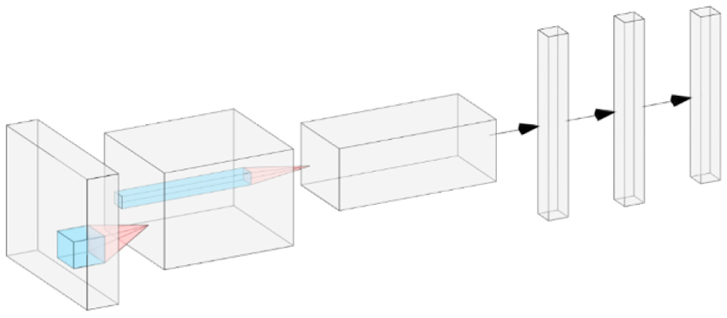
The architecture of convolution neural networks comprises feature selection in the first half and classifiers in the second half, as shown in Figure 2. However, the main difference is that traditional methods are conducted through manually designed feature selection mechanisms, such as Histogram of Orientation Gradient (HOG), Local Binary Pattern (LBP), and Scale-Invariant Feature Transform (SIFT). For convolution neural networks, feature selection is conducted based on learning parameters and offsets of the convolutional, pooling, and activation function layers. The effects of the convolution kernels gained from learning are significantly better than those gained from the traditional method for feature selection.

Convolution neural networks are divided into the convolutional layer, pooling layer, and activation function layer. These layers are introduced as f.

2.1. Convolutional Layer

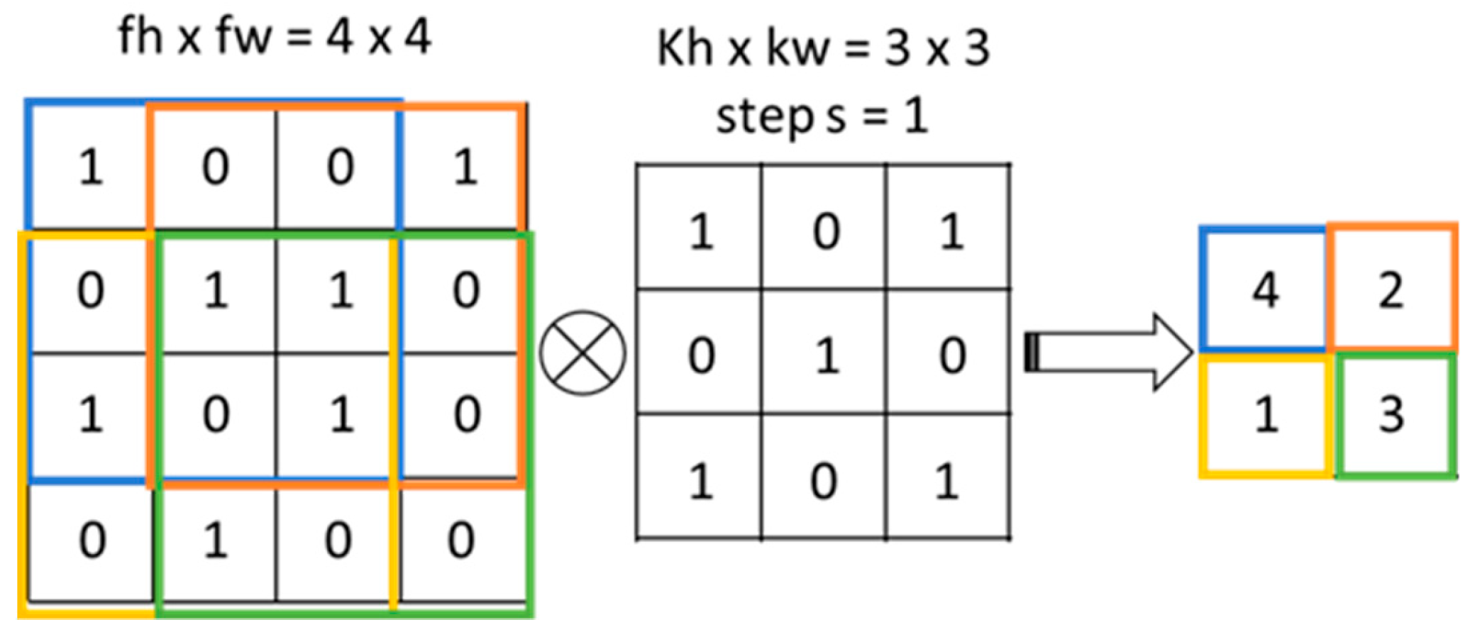
The convolutional layer is the most important part in convolution neural networks. The features are extracted through convolution kernels after learning, and then mapping from low-level features to high-level features is completed through superposition of multi-layer convolution kernels to achieve good effects. Figure 3 is a schematic diagram with a step (s) of 1 and kernel ($K_h\times K_w$) of $3\times 3$ for a convolution operation of a$4\times 4$ feature map ($f_h\times f_w$), and the operation is shown in Equations (3) and (4). The convolution result is shown as follows:

$$Y_{IJ}={{\displaystyle \sum }}_{i=0}^{K_w}{{\displaystyle \sum }}_{j=0}^{K_h}{x}_{\left(I+i-1\right)\left(J+j-1\right)}\ast k_{ij}\mathrm{and}$$

(3)

$$\mathrm{h}\times \mathrm{w}=\left(\frac{fh-kh}{s}+1\right) \times \left(\frac{fw-kw}{s}+1\right).$$

(4)

2.2. Pooling Layer

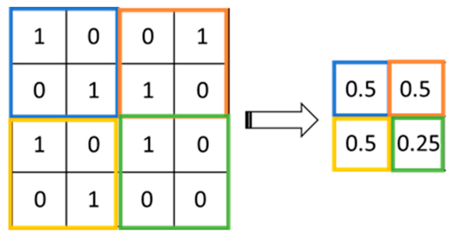
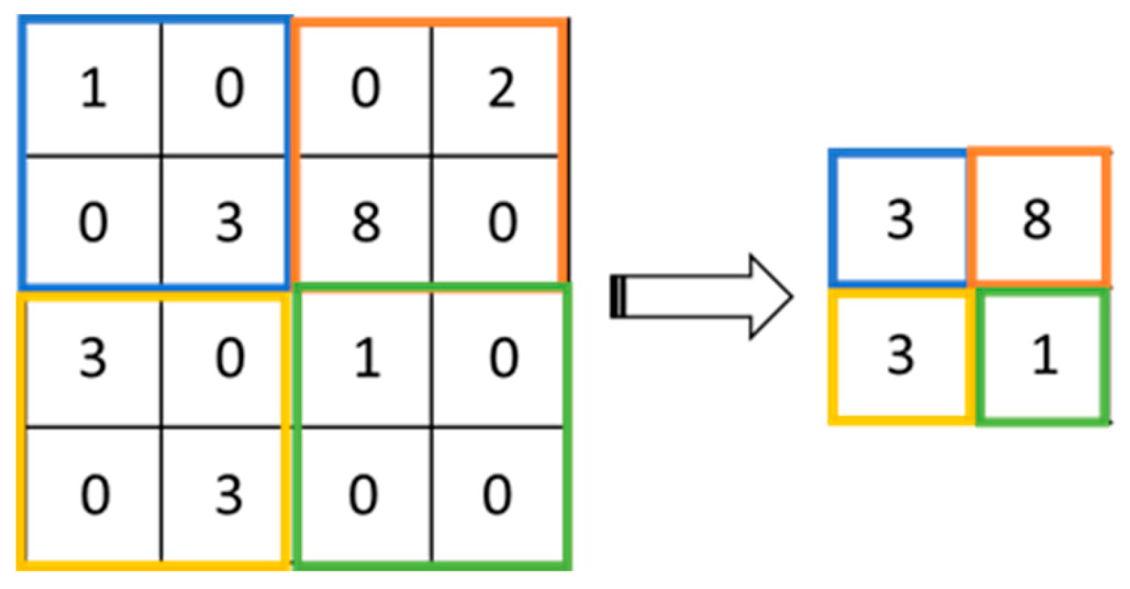
In general, two pooling operations are commonly used: average pooling and max pooling. Figure 4 shows the average pooling operation, which adds up the elements within the specified range and takes the average. Max pooling takes the maximum element within the range as a new value, which is shown in Figure 5.

2.3. Activation Function Layer

In order to increase the fitting ability of neural networks, an activation function layer is added to make the original linear neural networks fit nonlinear functions. Early researchers used sigmoid as the activation function layer. In training deep neural networks, due to features of the sigmoid function, the gradient approaches 0 in the functional saturation region, which results in the disappearance of the gradient and bottlenecks the training. Currently, a commonly used activation function layer is Rectified Linear Unit (ReLU), a piecewise function, where the gradient is kept at 1 in the region greater than 0 and is kept at 0 in the region smaller than 0. In addition to solving the disappearance of the gradient, ReLU can increase sparse neural networks and prevent overfitting. Current common activation functions are shown in

Table 2. Common activation functions.

Name	Functions	Derivatives
Sigmoid	$\mathsf{\sigma }\left(\mathsf{{\rm X}}\right)=\frac{1}{1+e^{-x}}$	$f^{\prime }\left(\mathsf{{\rm X}}\right)=f\left(\mathsf{{\rm X}}\right){\left(1-f\left(\mathsf{{\rm X}}\right)\right)}^2$
tanh	$\mathsf{\sigma }\left(\mathsf{{\rm X}}\right)=\frac{e^x-e^{-x}}{e^z+e^{-z}}$	$f^{\prime }\left(\mathsf{{\rm X}}\right)=1-f{\left(\mathsf{{\rm X}}\right)}^2$
ReLU	$f\left(\mathsf{{\rm X}}\right)=\{\begin{array}{c}0 if \mathsf{{\rm X}}<0\\ \mathsf{{\rm X}} \mathrm{if} \mathsf{{\rm X}}\ge 0\end{array}$	$f^{\prime }\left(\mathsf{{\rm X}}\right)=\{\begin{array}{c}0 if \mathsf{{\rm X}}<0\\ 1 \mathrm{if} \mathsf{{\rm X}}\ge 0\end{array}$
Leaky ReLU	$f\left(\mathsf{{\rm X}}\right)=\{\begin{array}{c}0.01\mathsf{{\rm X}} if \mathsf{{\rm X}}<0\\ \mathsf{{\rm X}} \mathrm{if} \mathsf{{\rm X}}\ge 0\end{array}$	$f^{\prime }\left(\mathsf{{\rm X}}\right)=\{\begin{array}{c}0.01 if \mathsf{{\rm X}}<0\\ 1 \mathrm{if} \mathsf{{\rm X}}\ge 0\end{array}$

.

3. The Proposed RQDNN

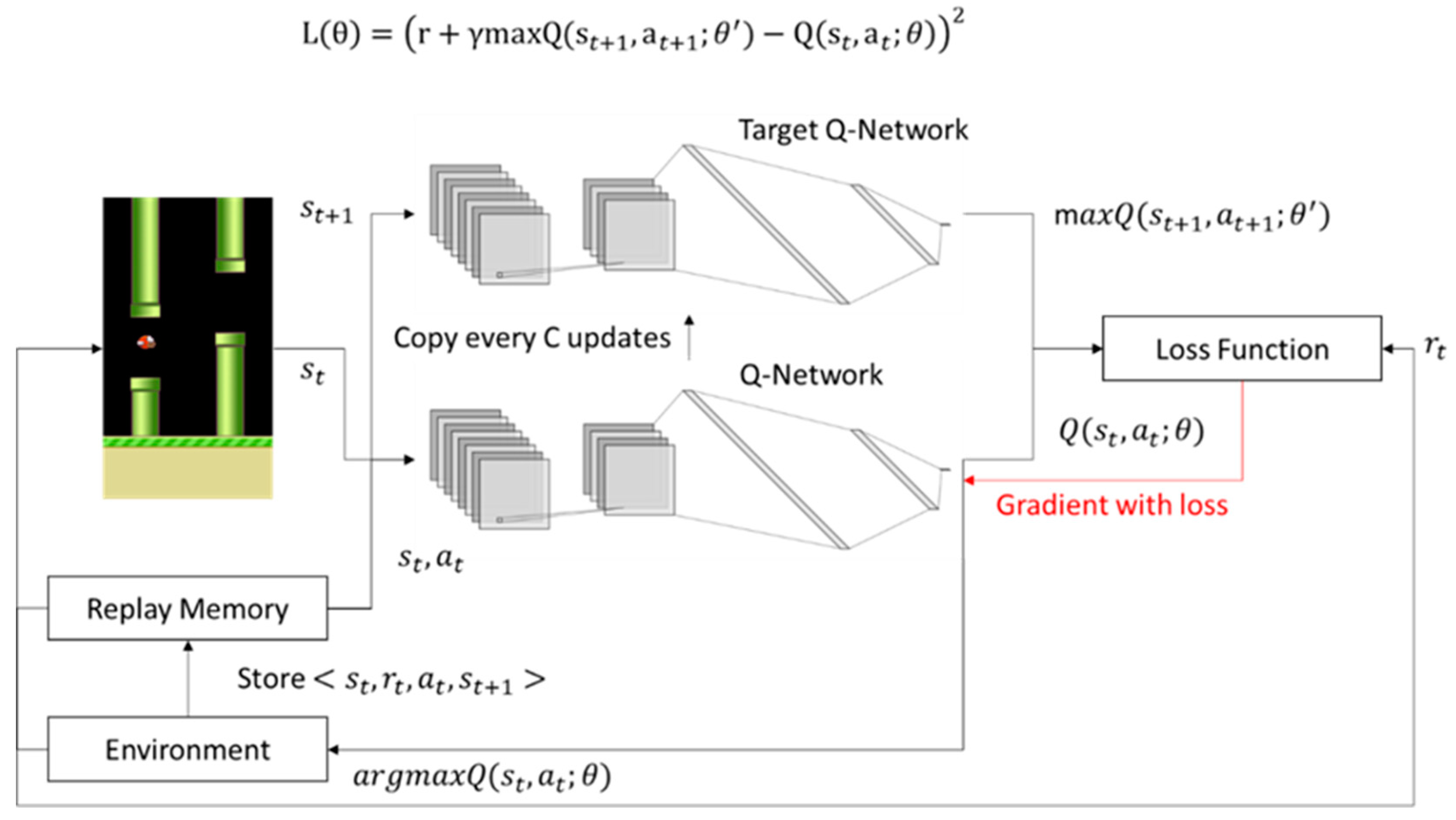
To reduce the hardware computing resources and training time of deep reinforcement learning, this study proposed the reinforcement Q-learning-based deep neural network (RQDNN), as shown in Figure 6. $S_t\mathrm{and}{S}_{t+1}$ are the input and output of the neural network, respectively, taking a reverse transfer to update neural network parameters, in which $\mathrm{L}\left(\theta \right)$ is the loss function of the RQDNN.

This section introduces the network architecture and operation flow of the RQDNN. Firstly, in order to train the algorithm stably, by reference of Mnih Nature DQN [3], this paper used a double-network architecture to estimate loss functions, and the loss function of the original DQN is as shown in Equation (5). After each parameter update, the original neural network will be changed when fitting the target, which leads to the algorithm being unable to converge stably.

$$\mathrm{Loss}={\displaystyle \sum }\left[{\left(R+\gamma ma{x}_{a^{\prime }}Q\left(S^{\prime },A^{\prime },\theta \right)-Q\left(S,A,\theta \right)\right)}^2\right].$$

(5)

Traditional DQN uses two groups of neural networks with identical architectures: Q-Network and Target Q-Network. The parameter of the Q-Network is $\theta$, while the parameter of the Target Q-Network is ${\theta }^{-}$. The loss function will be changed to Equation (6). In every training, only the parameters of the Q-Network are updated, and, after every 100 updates, the parameters of the Q-Network are copied to the Target Q-Network. In such a way, loss function calculations will be stable, accurate, and reduce the convergence time of algorithm.

$$\mathrm{Loss}={\displaystyle \sum }\left[{\left(R+\gamma ma{x}_{a^{\prime }}Q\left(S^{\prime },A^{\prime },{\theta }^{-}\right)-Q\left(S,A,\theta \right)\right)}^2\right]$$

(6)

DQN adopts a convolution neural network architecture, which contains three convolutional layers and two full connection layers. The architecture is simple, but, because of the features of convolution neural networks, the computing resources and time for training are greatly increased. Moreover, in the early training of the algorithm, convolution kernels cannot extract effective features, which greatly increases the training time of DQN. To solve this problem, a new network architecture, RQDNN, which combines DPCANet and Q-learning, was proposed in this study.

3.1. The Proposed DPCANet

The proposed DPCANet is an 8-layer neural network. The network architecture is shown in Figure 7, and the operation in each layer is described as follows:

● The first layer (input layer):

This layer has no operations, but it is responsible for pre-treatment of the input game pictures, which involves magnifying images to $80\times 80$ and recording the time it takes for convolution operation.

● The second and third layers (convolutional layers):

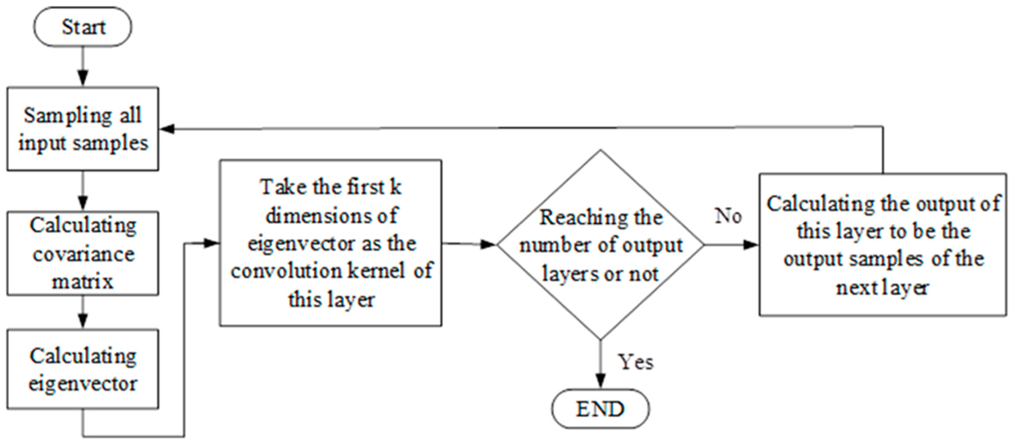
Both of these layers are convolutional layers. There are 8 convolutional layers on the second layer and 4 on the third layer. The size of the convolution kernels is $5\times 5$ with a step of 1. But, different from the parameters of convolution kernels in traditional convolution neural networks learned from algorithms, the parameters of the convolution kernels on both layers are gained from principal component analysis calculations. This calculation flow is as shown in Figure 8.

Before calculating the parameters of convolution kernels, firstly, images were collected through interaction with the games and models of random actions served as the training samples. There were a total of n training samples, which is indicated by $\mathrm{X}=\left\{x_1,x_2,x_3,\dots ,x_n\right\}$.

The first step is to sample $x_1$ in the range of $5\times 5$ and then flatten all blocks gained from sampling and splice them into a matrix $\widetilde{x_1},\widetilde{x_1}$, with a size of 25 × 25, calculated as Equation (7) where h and w are, respectively, the length and width of $x_1$, $k_h\mathrm{and}{k}_w$ are, respectively, the length and width of the convolution kernel, and s is the step. Next, in the same way, other samples are sampled to get the training set $\tilde{\mathrm{X}}=\left\{\widetilde{x_1},\widetilde{x_2},\widetilde{x_3},\dots ,\widetilde{x_n}\right\}$.

$$\left(k_h\times k_w\right)\times (\left(\frac{h-k_h}{s}+1\right)\times \left(\left(\frac{w-k_w}{s}+1\right)\right).$$

(7)

The second step is to calculate the covariance matrix of $\widetilde{x_1}$. Firstly, the mean m of $\tilde{\mathrm{X}}$ is calculated with a size of $1\times 5776$, subtracted m from $\widetilde{x_1}$ to get a new $\widetilde{x_1}$, and then $\widetilde{x_1}$ is multiplied by its own transport to get $\widetilde{x_1}{\widetilde{x_1}}^T$. The same operation is conducted for other training samples and then ${\tilde{\mathrm{X}}\tilde{\mathrm{X}}}^T=\left\{\widetilde{x_1}{\widetilde{x_1}}^T,\widetilde{x_2}{\widetilde{x_2}}^T,\widetilde{x_3}{\widetilde{x_3}}^T,\dots ,\widetilde{x_n}{\widetilde{x_n}}^T\right\}$ is obtained based on the calculations as shown in Equation (8). The size of the covariance matrix $\mathsf{\sigma }$ is $25\times 25$.

$$\mathsf{\sigma }=\frac{{{\displaystyle \sum }}_{i=1}^n\widetilde{x_i}{\widetilde{x_i}}^T}{(\left(\frac{h-k_h}{s}+1\right)\times \left(\left(\frac{w-k_w}{s}+1\right)\right)}.$$

(8)

Lastly, σ is entered into the Lagrange equation and an eigenvector size of $25\times 25$ is obtained. Then, take the first 8 dimensions as the parameters of the 8 convolution kernels on the second layer. The parameters of the 4 convolution kernels on the third layer can also be obtained through calculations of the above-mentioned steps. But, before calculating the convolution kernels on the third layer, a 2-layer convolution operation is conducted on $\mathrm{X}=\left\{x_1,x_2,x_3,\dots ,x_n\right\}$ to get ${\mathrm{X}}_{L2}=\left\{x_{11},x_{12},\dots ,x_{18},x_{21},x_{22},\dots ,x_{28},\dots ,x_{n8}\right\}$ and then the parameters of the third-layer convolution kernel are calculated with${\mathrm{X}}_{L2}$ as the new training sample set.

● The fourth layer (block-wise histograms layer):

After performing convolution operations on the second and third layers, the original input image will produce 32 feature maps ($1\times 8\times 4$) in total, and effects similar to multi-layer convolution neural networks can be obtained through superposition of the second and third layers. For the activation function layer, however, we used block-wise histograms to achieve nonlinear transformation of the original activation function layer. The specific operation process is shown below.

After the third layer is convolved, the feature map is used for binarization and is expressed as ${\mathrm{X}}_{L3}$, ${\mathrm{X}}_{L3}=\left\{x_{11},x_{12},\dots ,x_{14},x_{21},x_{22},\dots ,x_{24},\dots ,x_{84}\right\}$. Firstly, ${\mathrm{X}}_{L3}$ is grouped every 4 pieces, and n groups of feature maps are gained in total $x_n=\left\{x_{n1},x_{n2},x_{n2},x_{n4}\right\}$, where n is the number of convolution kernels on the second layer. Based on the operation shown in Equation (9), the size of $\widetilde{x_n},\widetilde{x_n}$ is $72\times 72$. Next, $\widetilde{x_n}$ is divided into four blocks $18\times 18$ in size, expressed as $\widetilde{x_{1n}},\widetilde{x_{2n}},\widetilde{x_{3n}},\widetilde{x_{4n}}$. The four blocks are used for histogram statistics and spliced into a 1024-dimensional vector. Next, other groups of feature maps are operated in the same way, and lastly, all of them are spliced into an 8192-dimensional eigenvector as the output of this layer.

$$\widetilde{x_n}={{\displaystyle \sum }}_{i=1}^4{2}^{4-i}{x}_{ni}.$$

(9)

● The fifth, sixth, and seventh layers (full connection layers):

The fifth, sixth, and seventh layers are full connection layers and the dimensions are, respectively, 8192, 4096, and 512, with operations the same as those of other normal, similar neutral networks.

● The eighth layer (output layer):

The eighth and last layer is the output layer. The output dimension is the number of actions that can be controlled by the games and was set as 2 in this paper.

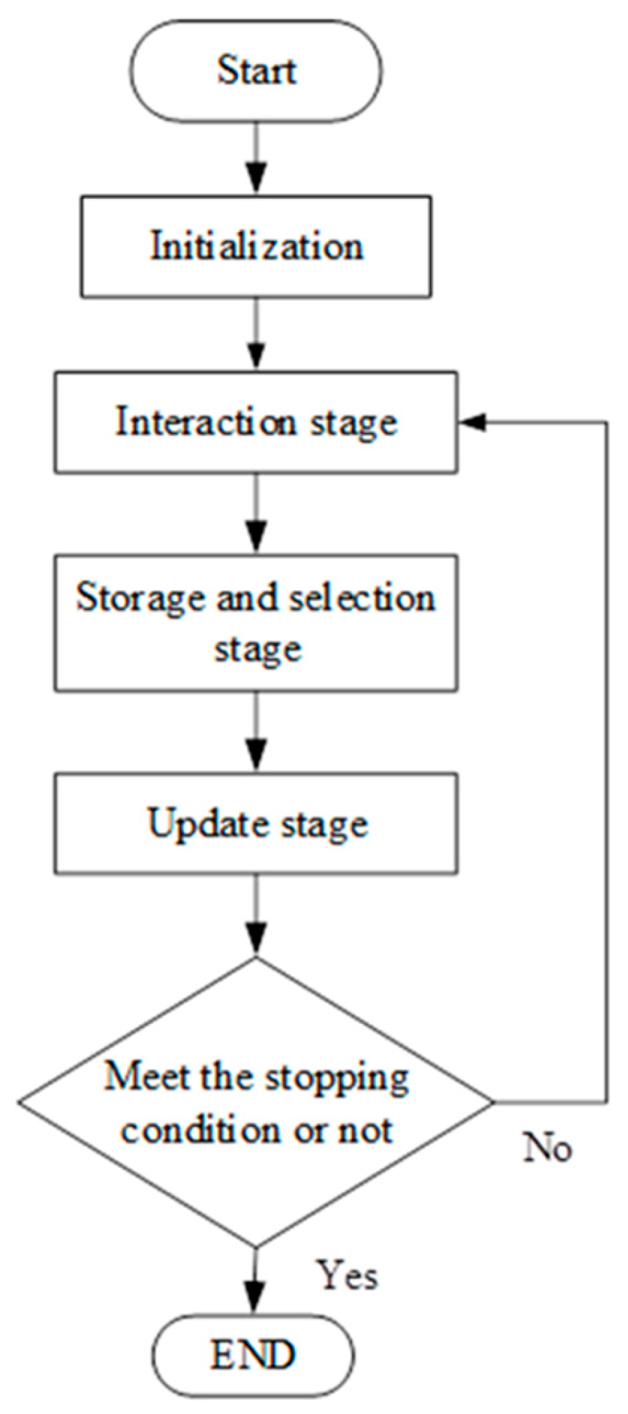
Next, the operation flow of DPCANet will be explained. The training flow comprises an interaction stage, storage and selection stage, and update stage, as shown in Figure 9.

3.2. The Proposed RQDNN

Before starting the major stage, initialization is conducted as the flow, as shown in Figure 10. In the beginning, an experience pool will be initialized. The experience pool D is responsible for all states and actions explored by RQDNN during training, and, at the update stage, experience will be randomly extracted from the experience pool to add into the parameter update. Next, Q-Network and Target Q-Network will be initialized, and the architectures of both networks are the same, as shown in Figure 7. At the update stage, parameter $\mathsf{\theta }$ of the Q-Network is the only one updated, and parameter ${\mathsf{\theta }}^{-}$ of the target Q-Network is synchronized with parameter $\mathsf{\theta }$ of the Q-Network upon every 100 update stages. Lastly, the environment will be initialized, and the initial state $s_0$ will be the output. Next are the circulation of interaction stage, storage and selection stage, and update stage, until the stopping condition is met. In this study, the stopping condition was to reach the specified survival time. The interaction stage, storage and selection stage, and update stage operated as below:

Upon completion of initialization, next comes the interaction stage with the flow, as shown in Figure 11. In the beginning, the states are taken from the environment, and the Q-values of all actions under $s_t$ shall be calculated by Q-Network. Next, $\epsilon greedy$ is used to select the action $a_t$ that will interact with the environment. If the probability is greater than $a_t$, the action will be selected randomly. In the end, a new state $s_{t+1}$ will be gained through the interaction between $a_t$ and the environment.

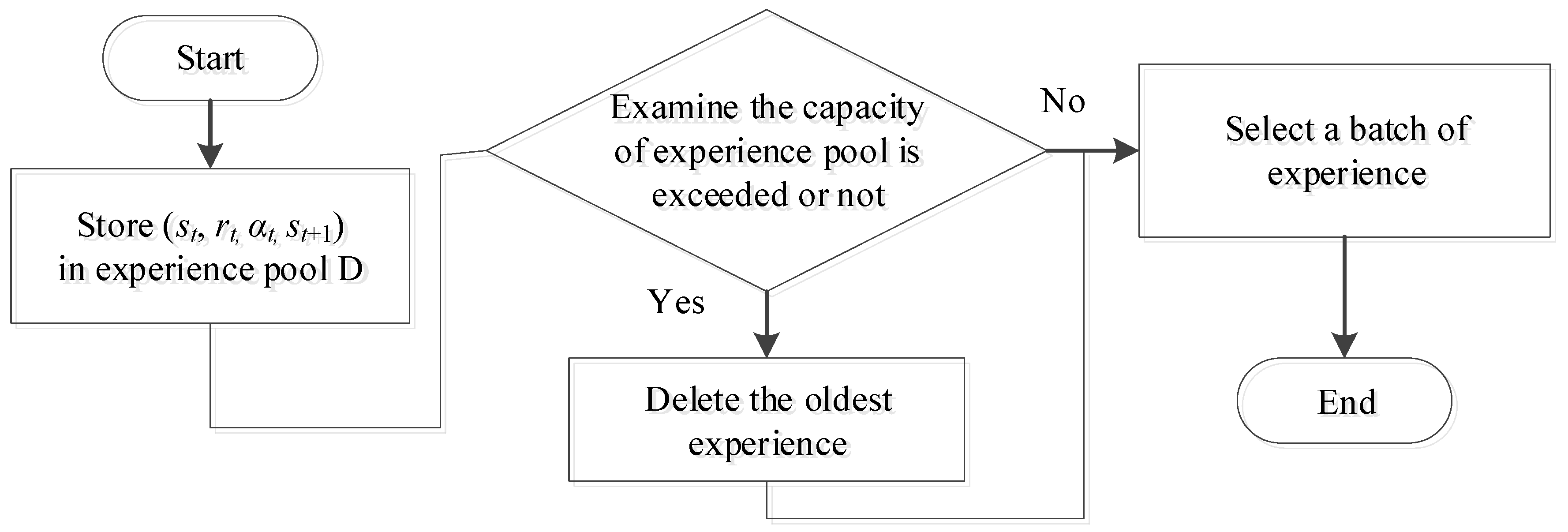
Next is the storage and selection stage. Algorithms related to Q-Learning are basically updated in single steps. Namely, the update is conducted for each interaction with the environment. Its advantages are its extremely high efficiency and the update can be done without completion of the entire flow. The disadvantages are that the strategies learned are simple to target and, once the game flow is changed, the effects of the strategies learned will be very poor. In order to solve this problem, DQN proposes replay memory, which stores all the experienced interactions in the experience pool D from interactions with environment. At the update stage, the experience most recently used in the interaction stage will not be directly used. Instead, a batch of experience randomly selected from the experience pool will be used. In this paper, the batch was set as 32, and the flow of storage and selection is shown in Figure 12.

The last is the update stage, and the flow is as shown in Figure 13. Upon selection from the experience pool, Equation (6) will be used to calculate loss function and the format of experience is $\langle s_t,r_t,a_t,s_{t+1}\rangle$. $\mathrm{Q}\left({\mathrm{s}}_t,{\mathrm{a}}_t;\theta \right)$ and $\mathrm{maxQ}\left({\mathrm{s}}_{t+1},{\mathrm{a}}_{t+1};{\theta }^{\prime }\right)$ are calculated through Q-Network and Target Q-Network and, after that, the state of ${\mathrm{s}}_{t+1}$ is examined, and r is given as the reward. When the barrier is successfully passed, r = 1, otherwise r = –1, and in the state of persistent existence, r = 0.1. Next, the loss function $\mathrm{L}\left(\mathsf{\theta }\right)$ can be calculated. The random gradient reduction shall be used to update parameter $\mathsf{\theta }$ of the Q-Network, and then parameter ${\mathsf{\theta }}^{-}$ of the target Q-Network is synchronized with parameter $\mathsf{\theta }$ of the Q-Network upon every 100 update stages.

Based on the above-mentioned stages, the proposed RQDNN can effectively learn to determine the playing strategy. The training time and hardware resources consumed in RQDNN are much less than those of DQN.

4. Experimental Results

In order to evaluate the effectiveness of the method proposed in this study, performance comparisons of different convolution layers and the two games (i.e., Flappy Bird and Atari Breakout) are implemented.

4.1. Evaluation of Different Convolution Layers in DPCANet

In this study, the proposed DPCANet replaced the traditional convolutional neural network (CNN) for extracting image features. DPCANet adopted a principal component analysis to calculate convolution kernel parameters, which can significantly reduce the computation time. In this subsection, the Modified National Institute of Standards and Technology (MNIST) database was used to test the network performances of different convolution layers. The MNIST dataset consists of grayscale images of handwritten digits 0–9. One thousand samples were used for training and testing in DPCANet. The experimental results are shown in

Table 3. Performance evaluation of different convolution layers.

	1st Layer Dimension of Convolution	2nd Layer Dimension of Convolution	3rd Layer Dimension of Convolution	4th Layer Dimension of Convolution	Testing Error Rate	Computation Time per Image (s)
Network 1	8	NaN	NaN	NaN	5.5%	0.12
Network 2	8	4	NaN	NaN	4.1%	0.17
Network 3	8	4	4	NaN	4.6%	0.22
Network 4	8	4	4	4	4.8%	0.34

. In this table, the performance of network 2 was better than that of the other networks. In addition, more convolutional layers increased the computing time and could not improve the accuracy during fixed iterations. Therefore, the architecture of network 2 was used to extract the features of game images.

4.2. The Flappy Bird Game

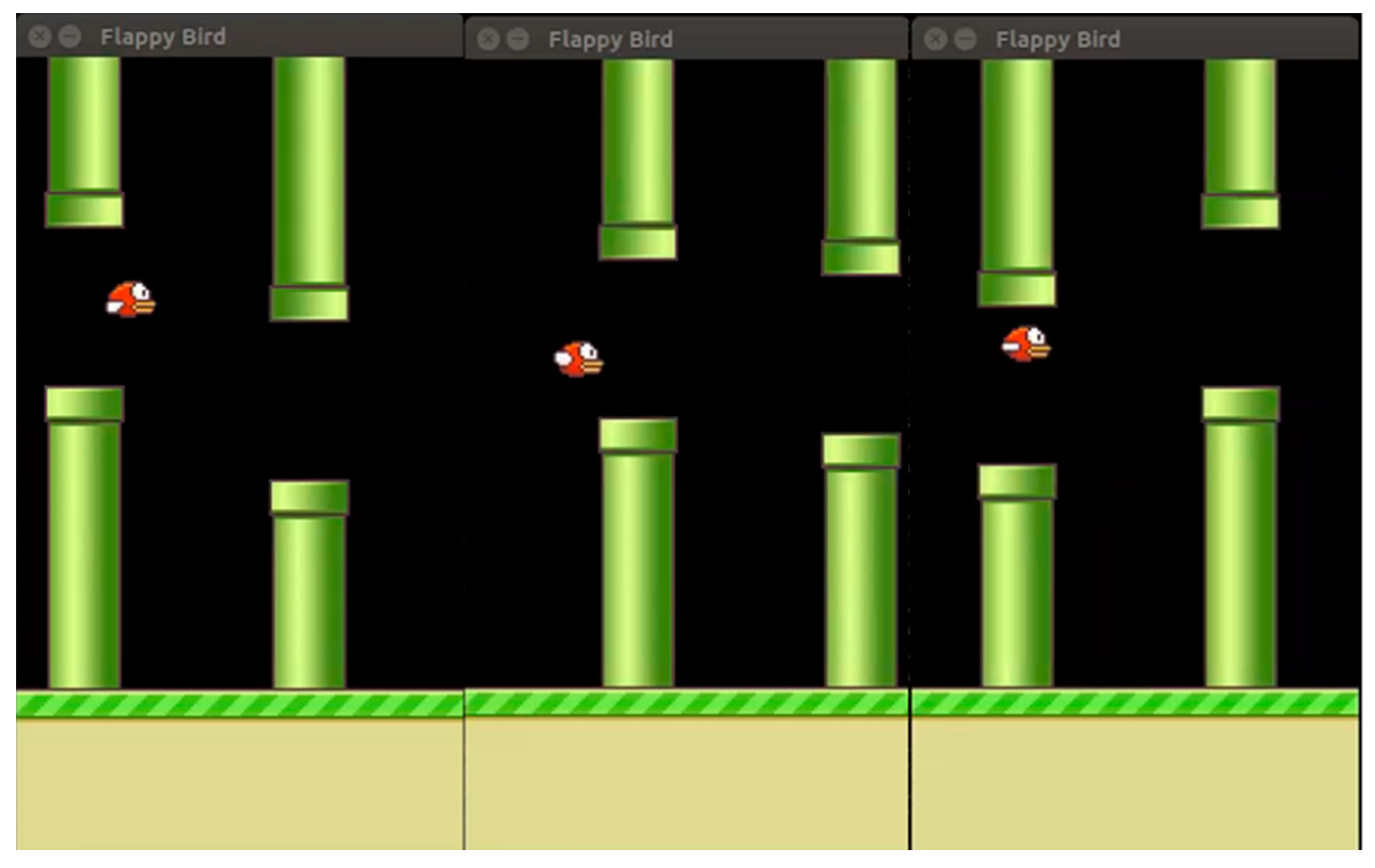
The Flappy Bird game is as shown in Figure 14. In this game, a player can manipulate the bird in the picture to continuously fly past water pipes. This game seems easy as there are only two actions: flying or not flying. But the position and length of the water pipes in the picture are completely random; thus, the state space is very huge. Such a relationship was fitted to verify the effectiveness of RQDNN.

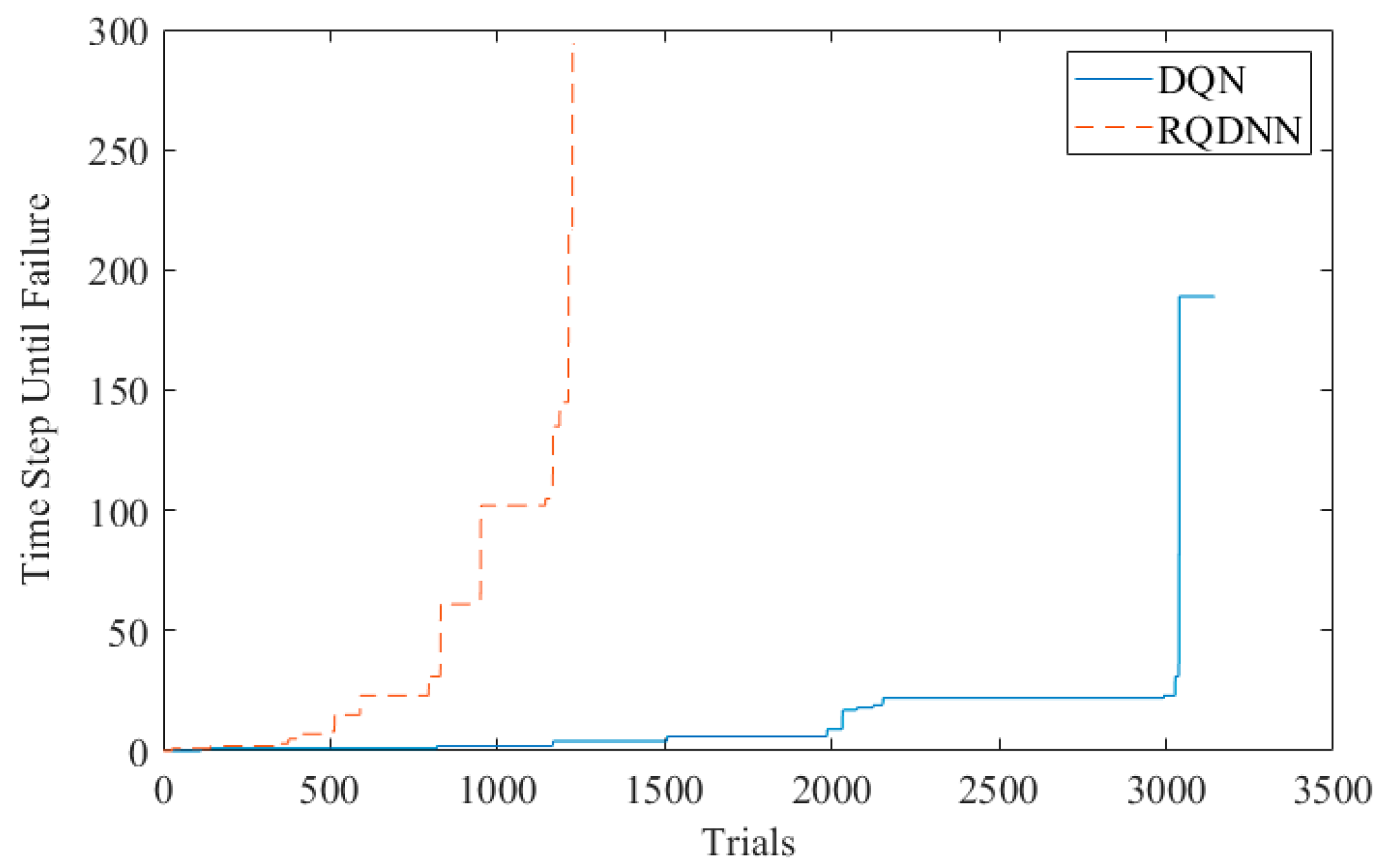
Next is the comparison of training and test results between the proposed RQDNN and DQN [2]. Firstly, the used hardware configurations for training are introduced, as shown in

Table 4. Hardware configurations of RQDNN and DQN [2]

	RQDNN	DQN [2]
CPU	Intel Xeon E3-1225	Intel Xeon E3-1225
GPU	None	GTX 1080Ti
Training time	2 h	5 h

. The training results are shown in Figure 15. This figure shows that the training time of RQDNN was shorter than DQN [2]. Moreover, the external computing resources in the proposed RQDNN did not require accelerated computing of the Graphics Processing Unit (GPU).

Here, we set passing 200 water pipes as the condition for successful training. In Figure 15, the rewards were given at the 400th and the 1200th trials using RQDNN and DQN, respectively. In addition, the proposed RQDNN required only 1213 trials to achieve successful training, while DQN required 3145 trials.

Next, the testing results were compared. If $\epsilon$ was set as 0, then the gained results are shown in Table 4 through 10 executions. The scores of the human player were gained from tests done by human players. In

Table 5. Testing results of the Flappy Bird game using various methods.

	Min	Max	Mean
Proposed method	223	287	254.2
V. Mnih [2]	176	234	213.4
Human player	10	41	21.6

, the gained score of the proposed method was better than that gained in the DQN proposed by Mnih [2] and significantly better than that gained by human players.

4.3. The Atari Breakout Game

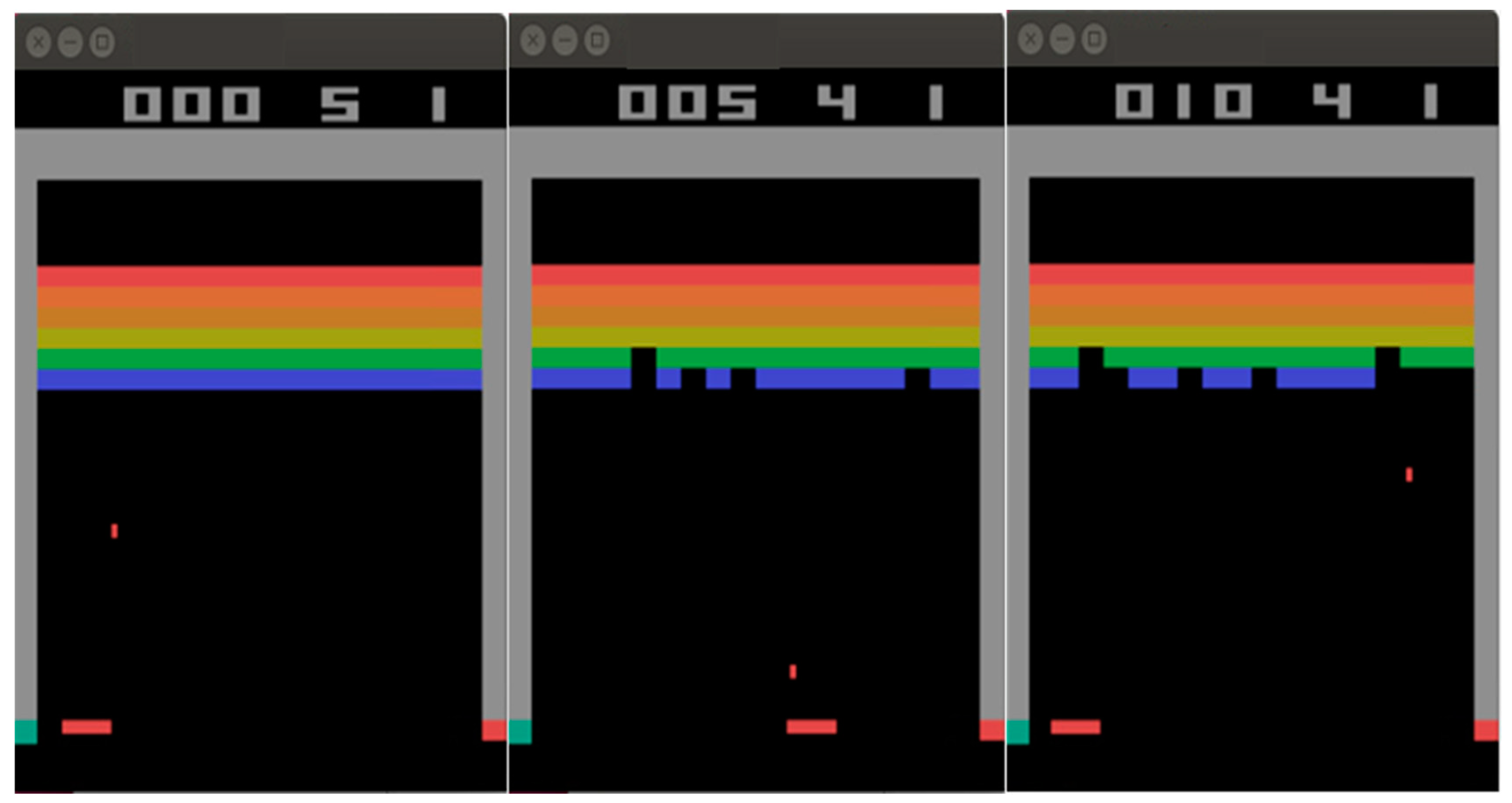
In Breakout, six bricks are arranged on the first third of the screen. A ball moves straight around the screen and bounces off the top and sides of the screen. When a brick is hit, the ball bounces, and the brick is destroyed. The player has a paddle that moves horizontally to reflect the ball and destroy all the bricks. There are five chances in a game. If the ball crosses the racket, the player will lose a chance. The Atari Breakout game is as shown in Figure 16.

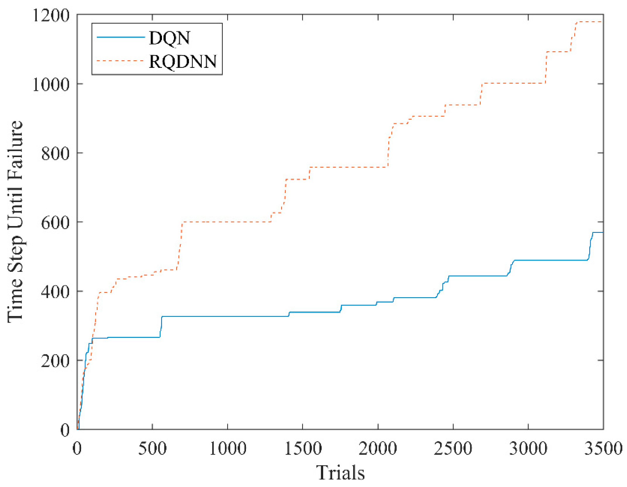
In this game, 3500 trials were set as the complete training condition for training process. The training results of the proposed RQDNN and DQN are shown in Figure 17. This figure shows that the proposed method had a faster convergence rate than DQN in playing the Breakout game. After 3500 trials, the proposed RQDNN kept 1179 time steps to play Breakout, while DQN only kept 570 time steps. The experimental results showed that the proposed RQDNN can keep a longer playing time than DQN in the Breakout game.

5. Conclusions and Future Work

In this study, a Reinforcement Q-Learning-based Deep Neural Network (RQDNN) was proposed for playing a video game. The proposed RQDNN comprised DPCANet and Q-learning to determine the playing strategy of video games. Video game images were used as the inputs. DPCANet was used to initialize the parameters of convolution kernels, to obtain good rewards, and to shorten the convergence time in training process. The reinforcement Q-learning method was used to capture the image features automatically and implement game control strategies. Experimental results showed that the scores of the proposed RQDNN were better than those of human players and other deep reinforcement learning algorithms. In addition, the training time of the proposed RQDNN was also far less than that of other deep reinforcement learning algorithms. Moreover, the proposed architecture did not require GPU to accelerate computation and needed less computing resources than traditional deep reinforcement learning algorithms.

Although the architecture of the proposed method replaces the convolutional and pooling layers of the original convolution neural network, the block-wise histogram layer used for the activation function layer is not good architecture. In addition to large dimensions, external feature combinations were also improved. In future work, we will focus on using kernel principal component analysis and other nonlinear methods to generate convolution kernels and improve the performance of deep reinforcement learning.

References

1. Togelius, J.; Karakovskiy, S.; Baumgarten, R. The 2009 Mario AI Competition. In Proceedings of the IEEE Congress on Evolutionary Computation, Barcelona, Spain, 18–23 July 2010. [Google Scholar] [CrossRef]
2. Mnih, V.; Kavukcuoglu, K.; Silver, D.; Graves, A.; Antonoglou, I.; Wierstra, D.; Riedmiller, M.A. Playing Atari with Deep Reinforcement Learning. arXiv 2013, arXiv:1312.5602. [Google Scholar]
3. Mnih, V.; Kavukcuoglu, K.; Silver, D.; Rusu, A.A.; Veness, J.; Bellemare, M.G.; Graves, A.; Riedmiller, M.A.; Fidjeland, A.; Ostrovski, G.; et al. Human-level control through deep reinforcement learning. Nature 2015, 518, 529–533. [Google Scholar] [CrossRef] [PubMed]
4. Schaul, T.; Quan, J.; Antonoglou, I.; Silver, D. Prioritized Experience Replay. arXiv 2016, arXiv:1511.05952. [Google Scholar]
5. Hasselt, H.v.; Guez, A.; Silver, D. Deep reinforcement learning with double Q-Learning. In Proceedings of the Thirtieth AAAI Conference on Artificial Intelligence (AAAI’16), Phoenix, AZ, USA, 12–17 February 2016. [Google Scholar]
6. Wang, Z.; Schaul, T.; Hessel, M.; Hasselt, H.V.; Lanctot, M.; Freitas, N.D. Dueling Network Architectures for Deep Reinforcement Learning. arXiv 2015, arXiv:1511.06581. [Google Scholar]
7. Li, D.; Zhao, D.; Zhang, Q.; Chen, Y. Reinforcement Learning and Deep Learning Based Lateral Control for Autonomous Driving. IEEE Comput. Intell. Mag. 2019, 14, 83–98. [Google Scholar] [CrossRef]
8. Martinez, M.; Sitawarin, C.; Finch, K.; Meincke, L. Beyond Grand Theft Auto V for Training, Testing and Enhancing Deep Learning in Self Driving Cars. arXiv 2017, arXiv:1712.01397. [Google Scholar]
9. Yu, X.; Lv, Z.; Wu, Y.; Sun, X. Neural Network Modeling and Backstepping Control for Quadrotor. In Proceedings of the 2018 Chinese Automation Congress (CAC), Xi’an, China, 30 November–2 December 2018. [Google Scholar] [CrossRef]
10. Kersandt, K.; Muñoz, G.; Barrado, C. Self-training by Reinforcement Learning for Full-autonomous Drones of the Future. In Proceedings of the 2018 IEEE/AIAA 37th Digital Avionics Systems Conference (DASC), London, UK, 23–27 September 2018. [Google Scholar] [CrossRef]
11. Lecun, Y.; Bottou, L.; Bengio, Y.; Haffner, P. Gradient-based learning applied to document recognition. Proc. IEEE 1998, 86, 2278–2324. [Google Scholar] [CrossRef] [Green Version]
12. Krizhevsky, A.; Sutskever, I.; Hinton, G.E. ImageNet classification with deep convolutional neural networks. In Proceedings of the 25th International Conference on Neural Information Processing Systems, Lake Tahoe, NV, USA, 3–6 December 2012. [Google Scholar]
13. Simonyan, K.; Zisserman, A. Very Deep Convolutional Networks for Large-Scale Image Recognition. arXiv 2014, arXiv:1409.1556. [Google Scholar]
14. Szegedy, C.; Liu, W.; Jia, Y.; Sermanet, P.; Reed, S.; Anguelov, D.; Erhan, D.; Vanhoucke, V.; Rabinovich, A. Going deeper with convolutions. In Proceedings of the 2015 IEEE Conference on Computer Vision and Pattern Recognition (CVPR), Boston, MA, USA, 7–12 June 2015. [Google Scholar] [CrossRef]
15. He, K.; Zhang, X.; Ren, S.; Sun, J. Deep Residual Learning for Image Recognition. In Proceedings of the 2016 IEEE Conference on Computer Vision and Pattern Recognition (CVPR), Las Vegas, NV, USA, 27–30 June 2016. [Google Scholar] [CrossRef]
Figure 1. The structure of reinforcement learning.
Electronics 08 01128 g001
Figure 2. Schematic diagram of convolution neural networks.
Electronics 08 01128 g002
Figure 3. Schematic diagram of convolution kernel operation.
Electronics 08 01128 g003
Figure 4. Schematic diagram of average pooling.
Electronics 08 01128 g004
Figure 5. Schematic diagram of max pooling.
Electronics 08 01128 g005
Figure 6. Diagram of the reinforcement Q-learning-based deep neural network (RQDNN) algorithm.
Electronics 08 01128 g006
Figure 7. Diagram of the proposed DPCANet.
Electronics 08 01128 g007
Figure 8. Flowchart of parameter calculations of convolution kernels.
Electronics 08 01128 g008
Figure 9. Flowchart of deep principal component analysis network (DPCANet).
Electronics 08 01128 g009
Figure 10. Flowchart of initialization.
Electronics 08 01128 g010
Figure 11. Flowchart of the interaction stage.
Electronics 08 01128 g011
Figure 12. Flowchart of the storage and selection stage.
Electronics 08 01128 g012
Figure 13. Flowchart of the update stage.
Electronics 08 01128 g013
Figure 14. The Flappy Bird game.
Electronics 08 01128 g014
Figure 15. Comparison results of RQDNN and Deep Q-learning Network (DQN) [2] training with the Flappy Bird game.
Electronics 08 01128 g015
Figure 16. The Atari Breakout game.
Electronics 08 01128 g016
Figure 17. Comparison results of RQDNN and DQN [2] in the Breakout game.
Electronics 08 01128 g017