Review of the Comprehensive SAR Approach to Identify Scattering Mechanisms of Radar Backscatter from Vegetated Terrain

Abstract
:1. Introduction
2. Model-Based Polarimetric Decompositions and Their Limitation
3. Comprehensive SAR Approach
3.1. Forward Model
3.2. Multiparametric SAR Observation
4. Conclusions
Author Contributions
Funding
Conflicts of Interest
References
- Le Toan, T.; Laur, H.; Mougin, E.; Lopes, A. Multitemporal and dual-polarization observations of agricultural vegetation covers by X-band SAR images. IEEE Trans. Geosci. Remote Sens. 1989, 27, 709–718. [Google Scholar] [CrossRef]
- Zebker, H.A.; van Zyl, J.J.; Durden, S.L.; Norikane, L. Calibrated imaging radar polarimetry: Technique, examples, and applications. IEEE Trans. Geosci. Remote Sens. 1991, 29, 942–961. [Google Scholar] [CrossRef]
- Dubois, P.C.; van Zyl, J.; Engman, T. Measuring Soil Moisture with Imaging Radars. IEEE Trans. Geosci. Remote Sens. 1995, 33, 916–926. [Google Scholar] [CrossRef]
- Dobson, M.C.; Pierce, L.E.; Ulaby, F.T. Knowledge-based land-cover classification using ERS-1/JERS-1 SAR composites. IEEE Trans. Geosci. Remote Sens. 1996, 34, 83–99. [Google Scholar] [CrossRef]
- Le Toan, T.; Ribbes, F.; Wang, L.-F.; Floury, N.; Ding, K.-H.; Kong, J.-A.; Fujita, M.; Kurosu, T. Rice crop mapping and monitoring using ERS-1 data based on experiment and modeling results. IEEE Trans. Geosci. Remote Sens. 1997, 35, 41–56. [Google Scholar] [CrossRef]
- Cloude, S.R.; Pottier, E. An entropy based classification scheme for land applications of polarimetric SAR. IEEE Trans. Geosci. Remote Sens. 1997, 35, 68–78. [Google Scholar] [CrossRef]
- Shi, J.; Wang, J.; Hsu, A.Y.; O’Neil, P.E.; Engman, E.T. Estimation of bare surface soil moisture and surface roughness parameter using L-band SAR image data. IEEE Trans. Geosci. Remote Sens. 1997, 35, 1254–1266. [Google Scholar]
- Pierce, L.E.; Bergen, K.M.; Dobson, M.C.; Ulaby, F.T. Multitemporal land-cover classification using SIR-C/X-SAR imagery. Remote Sens. Environ. 1998, 63, 24–39. [Google Scholar] [CrossRef]
- Hajnsek, I.; Pottier, E.; Cloude, S.R. Inversion of surface parameters from Polarimetric SAR. IEEE Trans. Geosci. Remote Sens. 2003, 41, 724–744. [Google Scholar] [CrossRef]
- Koay, J.-Y.; Tan, C.-P.; Lim, K.-S.; Bakar, S.; Ewe, H.-T.; Chuah, H.-T.; Kong, J.-A. Paddy fields as electrically dense media: Theoretical modeling and measurement comparisons. IEEE Trans. Geosci. Remote Sens. 2007, 45, 2837–2849. [Google Scholar] [CrossRef]
- Lucas, R.; Armston, J.; Fairfax, R.; Fensham, R.; Accad, A.; Carreiras, J.; Bunting, P.; Clewley, D.; Bray, S.; Metcalfe, D.; et al. An evaluation of the ALOS PALSAR L-band backscatter above ground biomass relationship Queensland, Australia: Impacts of surface moisture condition and vegetation structure. IEEE Trans. Geosci. Remote Sens. 2010, 3, 576–593. [Google Scholar] [CrossRef]
- Cloude, S.R. Uniqueness of target decomposition theorems in radar polarimetry. In Direct and Inverse Methods in Radar Polarimetry; Part 1, NATO-ARW; Boerner, W.M., Brand, H., Cram, L.A., Holm, W.A., Stein, D.E., Wiesbeck, W., Keydel, W., Giuli, D., Gjessing, D.T., Molinet, F.A., Eds.; Kluwer: Norwell, MA, USA, 1992; pp. 267–296. [Google Scholar]
- Van Zyl, J.J. Application of Cloude’s target decomposition theorem to Polarimetric imaging radar data. In Radar Polarimetry; SPIE-I748; SPIE: Bellingham, WA, USA, 1992; pp. 184–212. [Google Scholar]
- Freeman, A.; Durden, S.L. A three-component scattering model for Polarimetric SAR data. IEEE Trans. Geosci. Remote Sens. 1998, 36, 963–973. [Google Scholar] [CrossRef]
- Yamaguchi, Y.; Moriyama, T.; Ishido, M.; Yamada, H. Four-component scattering model for polarimetric SAR image decomposition. IEEE Trans. Geosci. Remote Sens. 2005, 43, 1699–1706. [Google Scholar] [CrossRef]
- Touzi, R. Target scattering decomposition in terms of roll invariant target parameters. IEEE Trans. Geosci. Remote Sens. 2007, 45, 73–84. [Google Scholar] [CrossRef]
- Freeman, A. Fitting a two-component scattering model to polarimetric SAR data from forests. IEEE Trans. Geosci. Remote Sens. 2007, 45, 2583–2592. [Google Scholar] [CrossRef]
- Van Zyl, J.J.; Arii, M.; Kim, Y. Model based decomposition of polarimetric SAR covariance matrices constrained for non-negative eigenvalues. IEEE Trans. Geosci. Remote Sens. 2011, 49, 3452–3459. [Google Scholar] [CrossRef]
- Arii, M.; van Zyl, J.J.; Kim, Y. Adaptive model-based decomposition of polarimetric SAR covariance matrices. IEEE Trans. Geosci. Remote Sens. 2011, 49, 1104–1113. [Google Scholar] [CrossRef]
- Jagdhuber, T.; Hajnsek, I.; Bronstert, A.; Papathanassiou, K.P. Soil moisture estimation under low vegetation cover using a multi-angular polarimetric decomposition. IEEE Trans. Geosci. Remote Sens. 2013, 51, 2201–2215. [Google Scholar] [CrossRef]
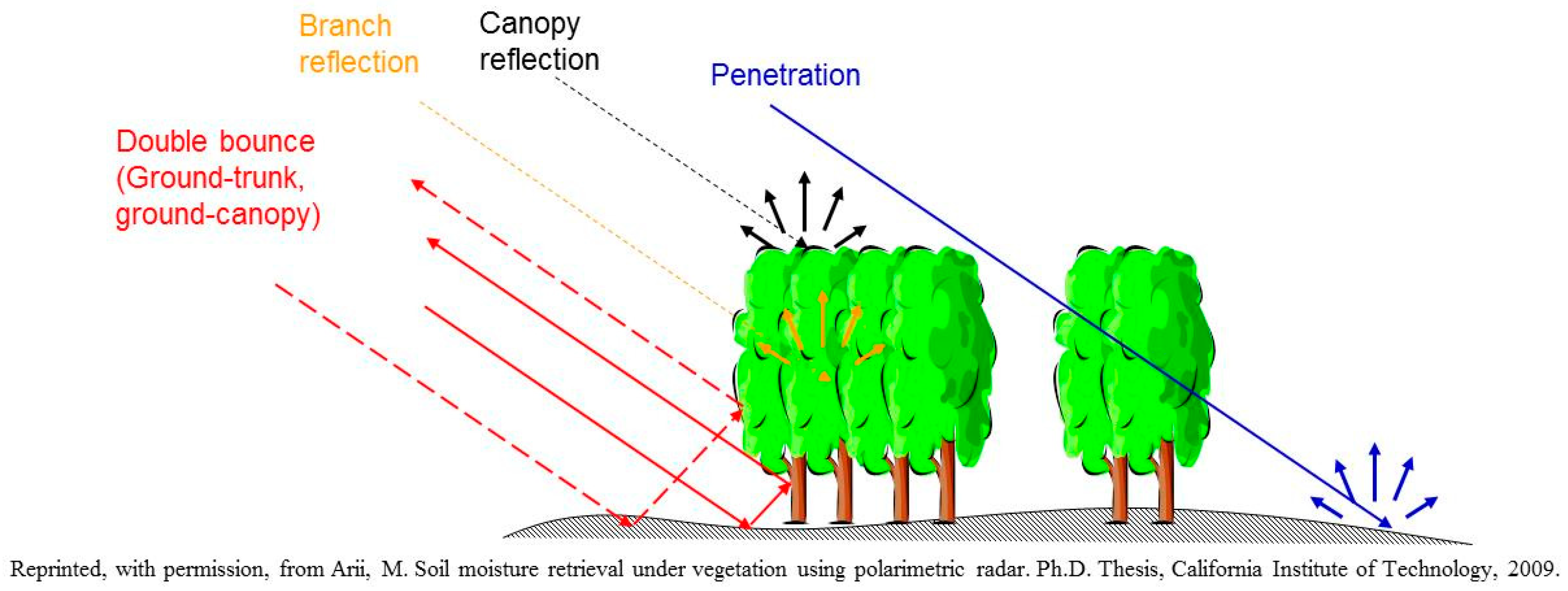
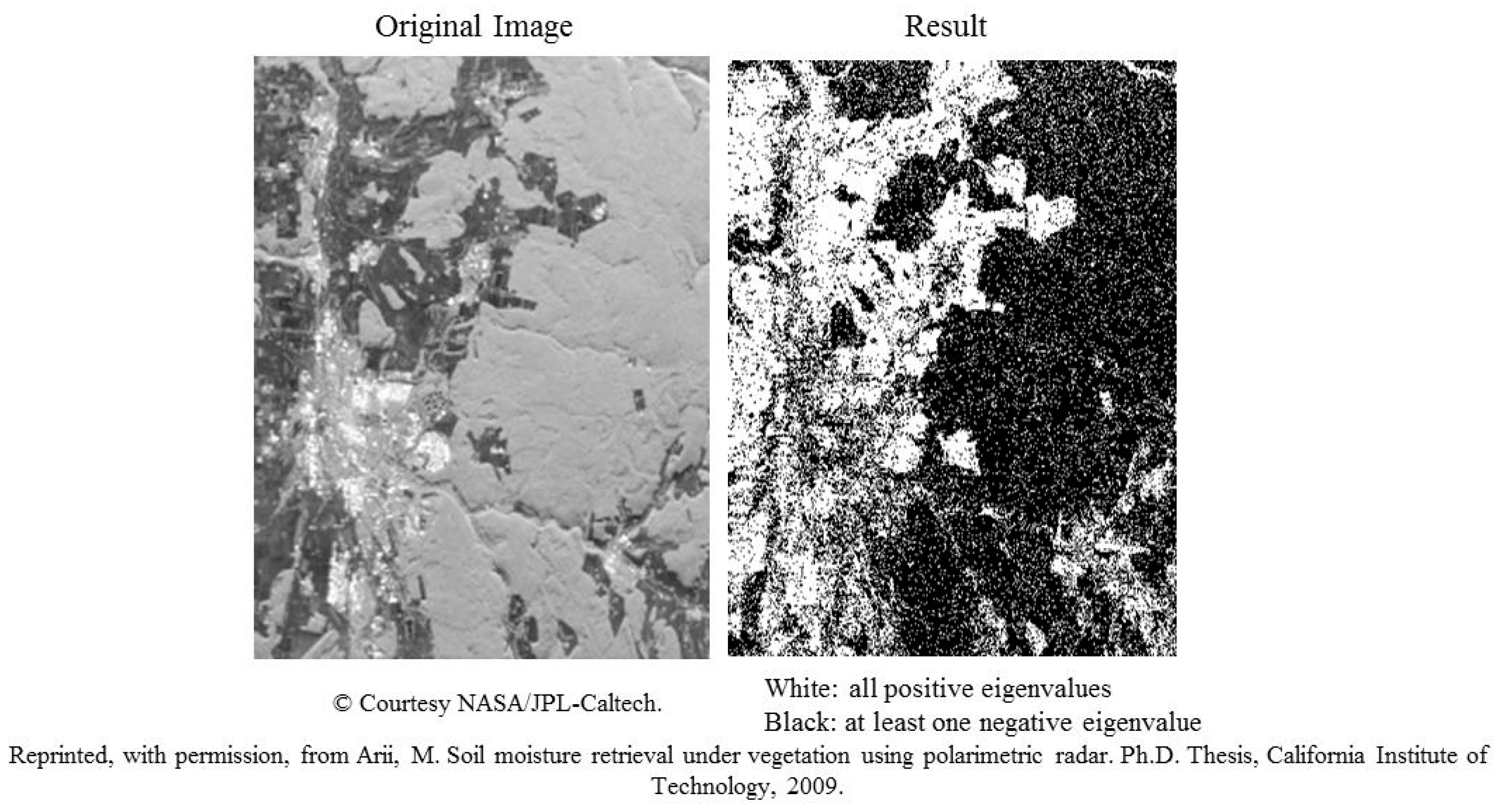
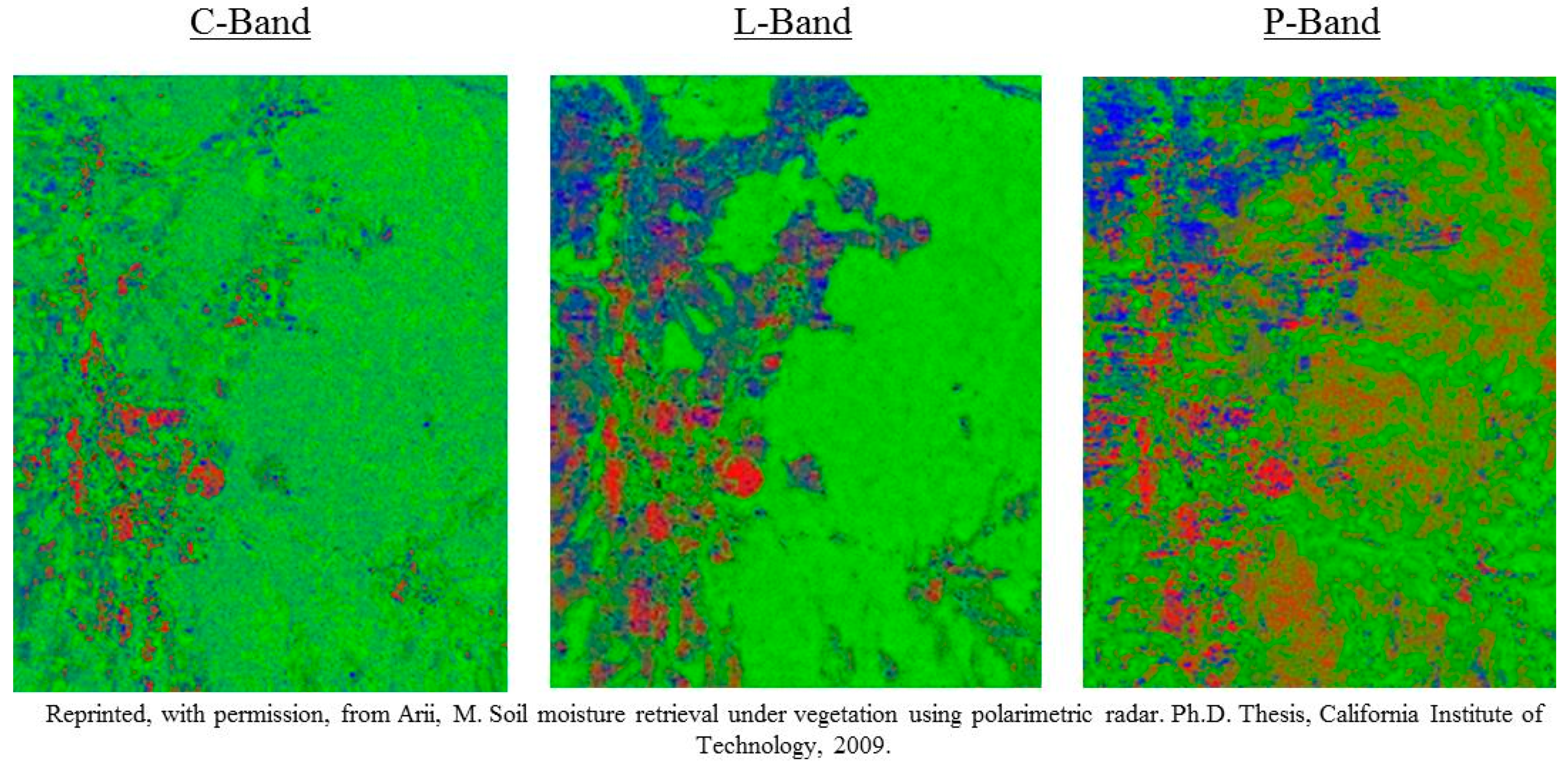
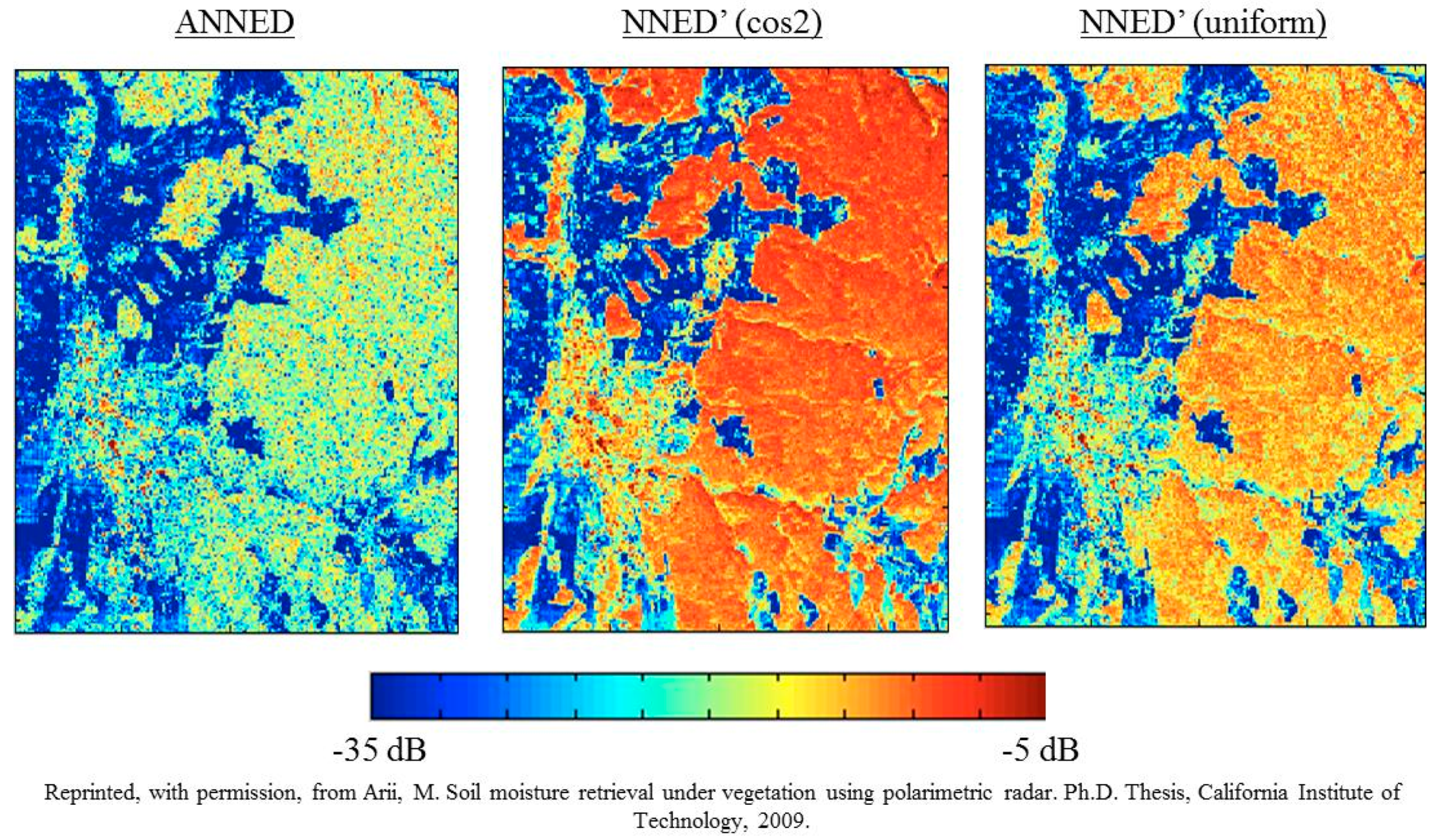
- Arii, M. Soil Moisture Retrieval under Vegetation Using Polarimetric Radar. Ph.D. Thesis, California Institute of Technology, Pasadena, CA, USA, 2009. [Google Scholar]
- Ishimaru, A. Wave Propagation and Scattering in Random Media; IEEE Press: New York, NY, USA, 1978. [Google Scholar]
- Bohren, C.F.; Huffman, D.R. Absorption and Scattering of Light by Small Particles; John Wiley & Sons: New York, NY, USA, 1983. [Google Scholar]
- Van Zyl, J.J.; Kim, Y. Synthetic Aperture Radar Polarimetry; Wiley: Hoboken, NJ, USA, 2011. [Google Scholar]
- Durden, S.L.; van Zyl, J.J.; Zebker, H.A. Modeling and observations of the radar polarization signatures of forested areas. IEEE Trans. Geosci. Remote Sens. 1989, 27, 290–301. [Google Scholar] [CrossRef]
- Durden, S.L.; Klein, J.D.; Zebker, H.A. Polarimetric radar measurements of a forested area near Mt. Shasta. IEEE Trans. Geosci. Remote Sens. 1991, 29, 444–450. [Google Scholar] [CrossRef]
- Arii, M.; Kitta, H.; Watanabe, T.; Yamada, H. Theoretical study of backscatter from rice paddy using discrete scatterer model. In Proceedings of the Asia-Pacific Conference on Synthetic Aperture Radar (APSAR), Tsukuba, Japan, 23–27 September 2013; pp. 27–30. [Google Scholar]
- Arii, M.; Komatsu, T.; Nishimura, T.; Watanabe, T.; Yamada, H.; Kobayashi, T. Theoretical characterization of X-band full polarimetric SAR data from rice paddies in terms of incidence angles. In Proceedings of the IEICE Technical Report, Niigata, Japan, 29 August 2014; Volume 114, pp. 67–72. [Google Scholar]
- Arii, M.; Watanabe, T.; Yamada, H. Sensitivity study of radar backscatter from boreal forest using discrete scatter model. In Proceedings of the IEEE International Geoscience and Remote Sensing Symposium, Munich, Germany, 22–27 July 2012; pp. 1425–1428. [Google Scholar]
- Watanabe, T.; Yamada, H.; Arii, M.; Park, S.-E.; Yamaguchi, Y. Model experiment of permittivity retrieval method for forested area by using Brewster’s angle. In Proceedings of the IEEE International Geoscience and Remote Sensing Symposium, Munich, Germany, 22–27 July 2012; pp. 1477–1480. [Google Scholar]
- Watanabe, T.; Yamada, H.; Arii, M.; Sato, R.; Park, S.-E.; Yamaguchi, Y. Study on moisture effects on polarimetric radar backscatter from forested terrain. IEICE Trans. Commun. 2014, 97, 2074–2082. [Google Scholar] [CrossRef]
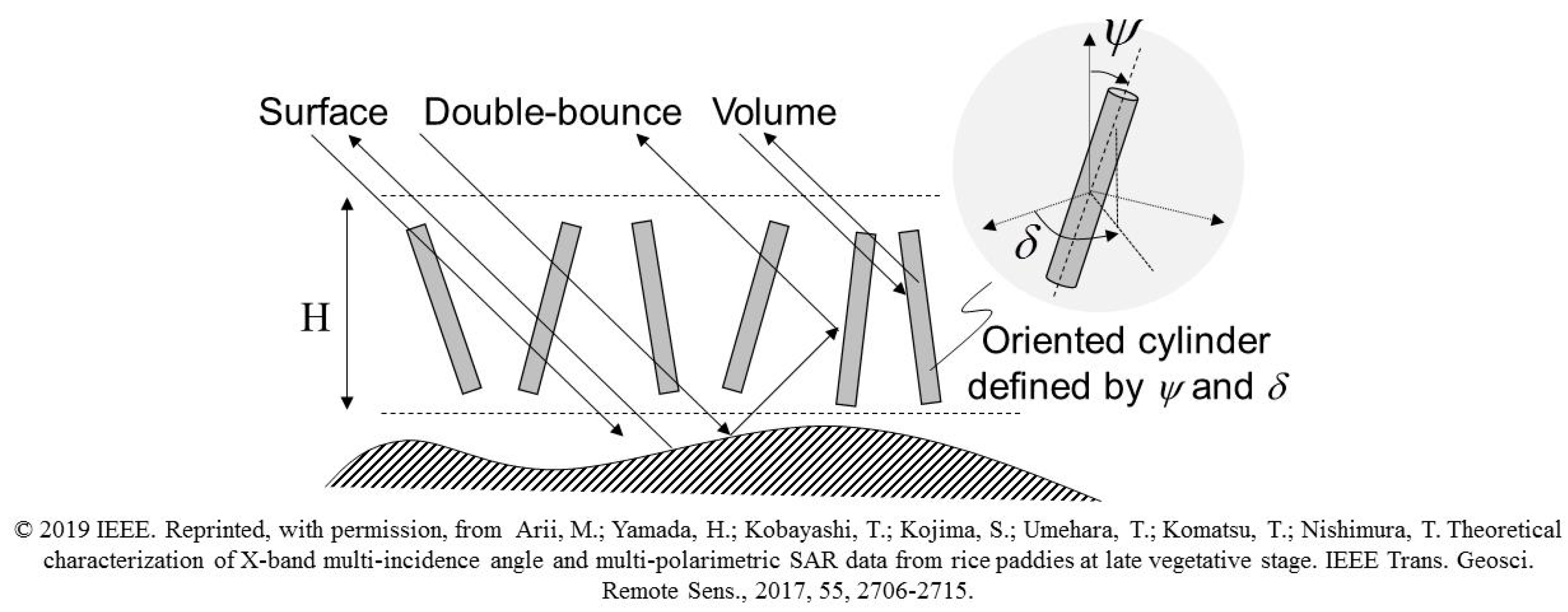
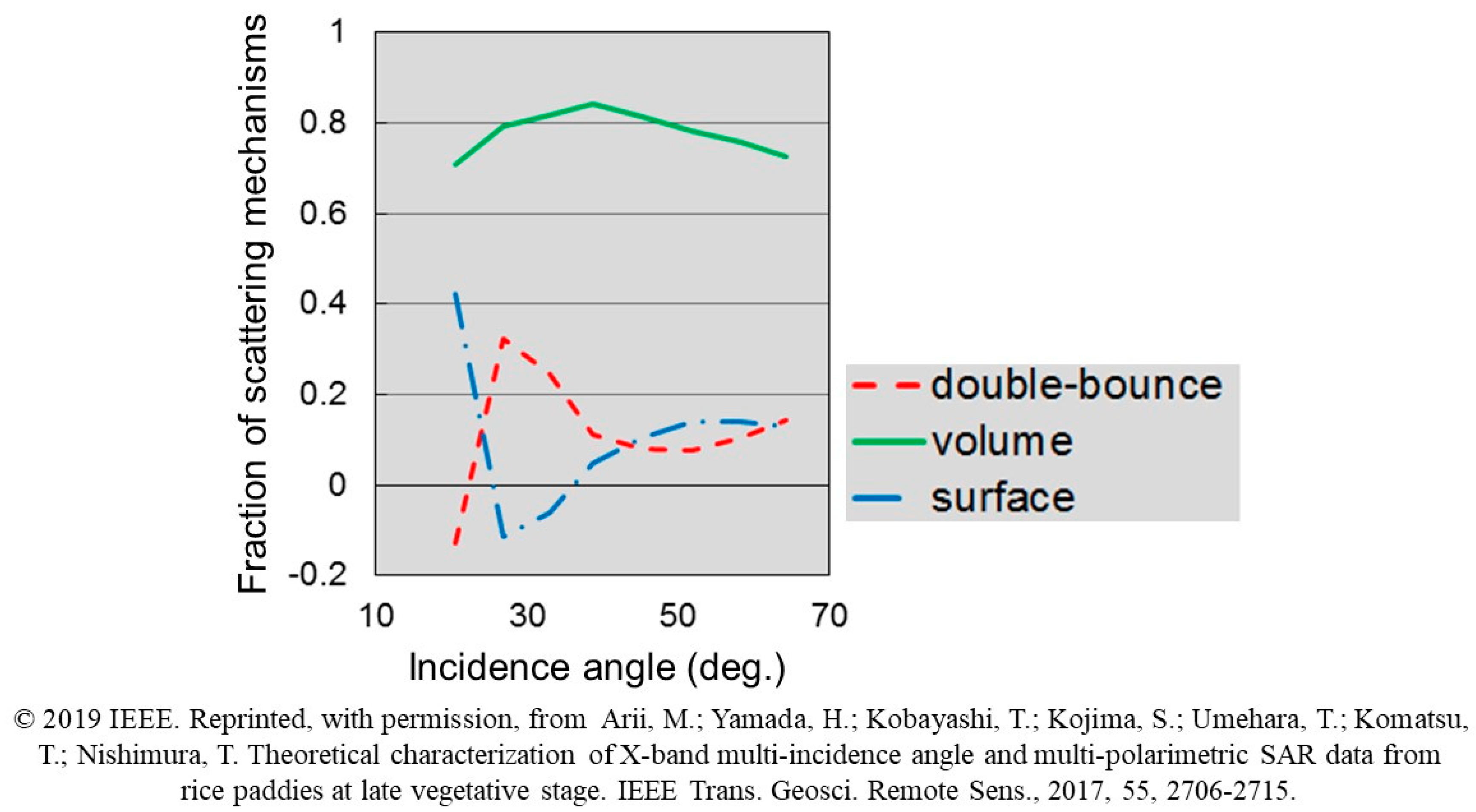
- Arii, M.; Yamada, H.; Kobayashi, T.; Kojima, S.; Umehara, T.; Komatsu, T.; Nishimura, T. Theoretical characterization of X-band multi-incidence angle and multi-polarimetric SAR data from rice paddies at late vegetative stage. IEEE Trans. Geosci. Remote Sens. 2017, 55, 2706–2715. [Google Scholar] [CrossRef]
- Arii, M.; Yamada, H. Rice paddy monitoring by L-band MIMP SAR Approach. In Proceedings of the IEEE International Geoscience and Remote Sensing Symposium (IGARSS), Fort Worth, TX, USA, 23–28 July 2017; pp. 2442–2445. [Google Scholar]
- Arii, M.; Yamada, H.; Ohki, M. Characterization of L-band MIMP SAR data from rice paddies at late vegetative stage. IEEE Trans. Geosci. Remote Sens. 2018, 56, 3852–3860. [Google Scholar] [CrossRef]
- Kim, S.; Arii, M.; Jackson, T. Modeling L-band synthetic aperture radar data through dielectric changes in soil moisture and vegetation over shrublands. IEEE J. Sel. Top. Appl. Earth Observ. Remote Sens. 2017, 10, 4753–4762. [Google Scholar] [CrossRef]
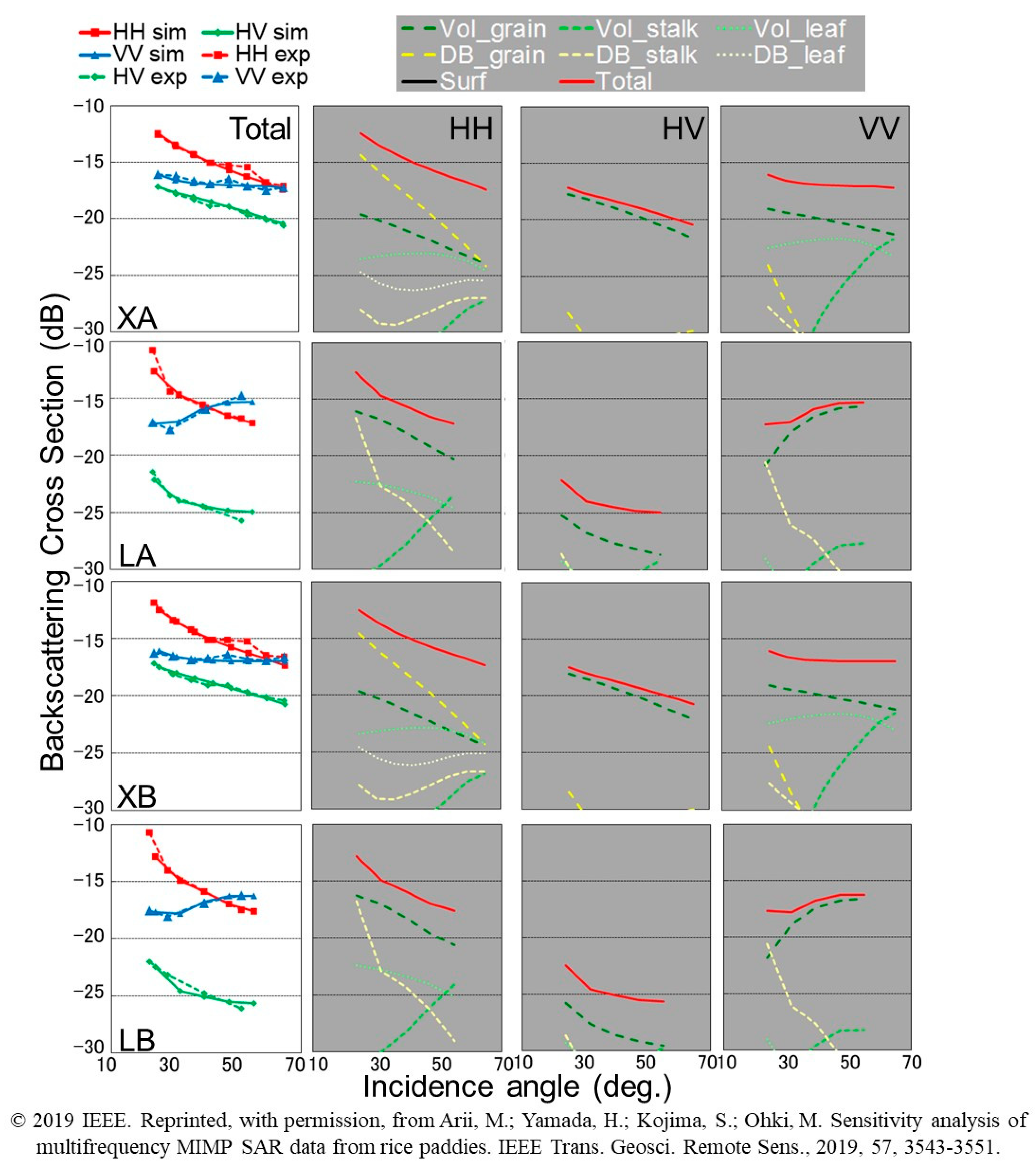
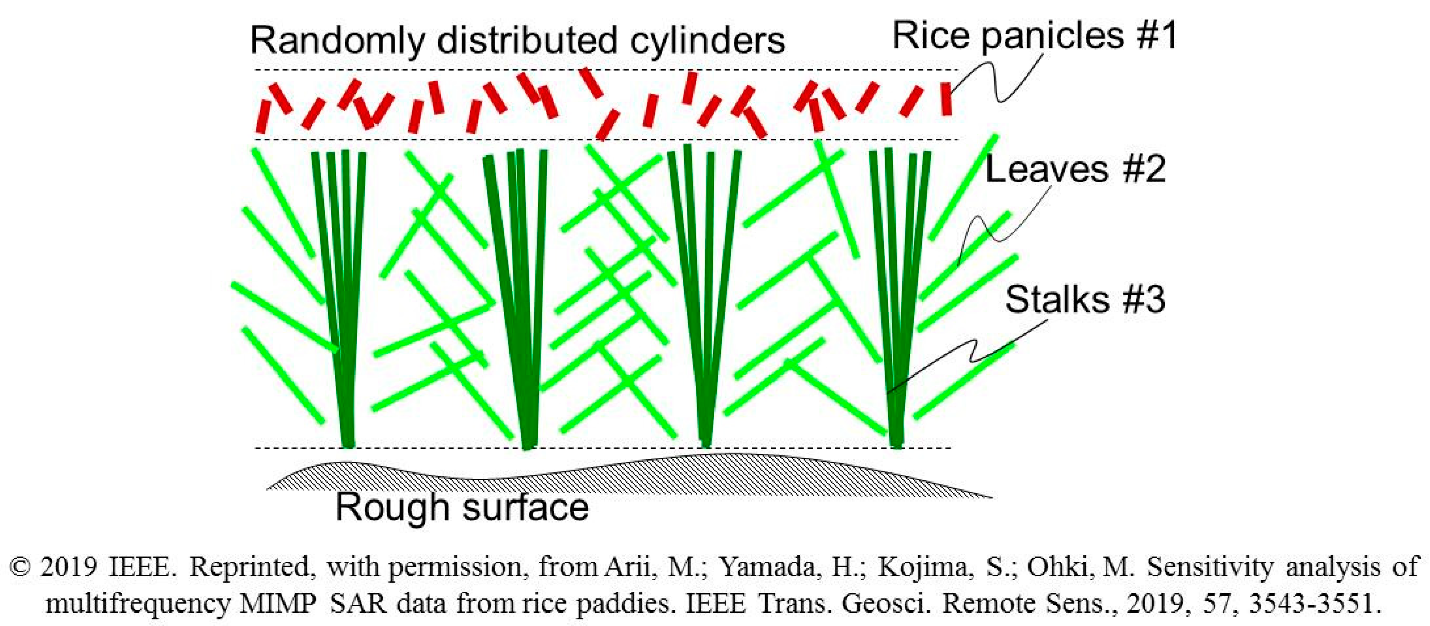
- Arii, M.; Yamada, H.; Kojima, S.; Ohki, M. Sensitivity analysis of multifrequency MIMP SAR data from rice paddies. IEEE Trans. Geosci. Remote Sens. 2019, 57, 3543–3551. [Google Scholar] [CrossRef]
- Arii, M.; van Zyl, J.J.; Kim, Y. A general characterization for polarimetric scattering from vegetation canopies. IEEE Trans. Geosci. Remote Sens. 2010, 48, 3349–3357. [Google Scholar] [CrossRef]
- Borgeaud, M.; Shin, R.T.; Kong, J.A. Theoretical models for polarimetric radar clutter. J. EM Waves Appl. 1987, 1, 73–91. [Google Scholar] [CrossRef]
- Chandrasekhar, S. Radiative Transfer; Dover: Mineola, NY, USA, 1960. [Google Scholar]
- Ulaby, F.T.; Sarabandi, K.; Mcdonald, K.C.; Whitt, N.W.; Dobson, M.C. Michigan Microwave Canopy Scattering Model (MIMICS); Rep. 022486-T-1; Radiation Laboratory, University of Michigan: Ann Arbor, MI, USA, 1988. [Google Scholar]
- Ulaby, F.; Sarabandi, K.; McDonald, K.; Whitt, M.; Dobson, C. Michigan microwave canopy scattering model. Int. J. Remote Sens. 1990, 11, 1223–1253. [Google Scholar] [CrossRef]
- MacDonald, K.C.; Dobson, M.C.; Ulaby, F.T. Using MIMICS to model multiangle and multitemporal backscatter from a walnut orchard. IEEE Trans. Geosci. Remote Sens. 1990, 28, 477–491. [Google Scholar] [CrossRef]
- Dobson, M.C.; Ulaby, F.T. Active microwave soil moisture research. IEEE Trans. Geosci. Remote Sens. 1986, GE-24, 23–36. [Google Scholar] [CrossRef]
- Tsang, L.; Kong, J.A.; Shin, R. Theory of Microwave Remote Sensing; Wiley: New York, NY, USA, 1985. [Google Scholar]
- Tsang, L.; Kong, J.A.; Ding, K.H. Scattering of Electromagnetic Waves; Vol. 1: Theory and Applications; Wiley: Hoboken, NJ, USA, 2000. [Google Scholar]
- Rice, S.O. Reflection of electromagnetic waves from slightly rough surfaces. Commun. Pure Appl. Math. 1951, 4, 351–378. [Google Scholar] [CrossRef]
- Van de Hulst, H.C. Light Scattering by Small Particles; Dover: Mineola, NY, USA, 1957. [Google Scholar]
- Ruck, G.T.; Barrick, D.E.; Stuart, W.D.; Krichbaum, C.K. Radar Cross Section Handbook; Plenum Press: New York, NY, USA, 1970. [Google Scholar]
- Ulaby, F.T.; Elachi, C. Radar Polarimetry for Geoscience Applications; Artech House: Norwood, MA, USA, 1990; pp. 92–101. [Google Scholar]
- Ulaby, F.T.; El-Rayes, M.A. Microwave dielectric spectrum of vegetation-Part II: Dual-dispersion model. IEEE Trans. Geosci. Remote Sens. 1987, GE-25, 550–557. [Google Scholar] [CrossRef]
- Ribbes, F.; Le Toan, F. Rice field mapping and monitoring with RADARSAT data. Int. J. Remote Sens. 1999, 20, 745–765. [Google Scholar] [CrossRef]
- Oh, Y.; Hong, S.; Kim, Y.; Hong, J.; Kim, Y. Polarimetric backscattering coefficients of flooded rice fields at L- and C-bands: Measurements, modeling, and data analysis. IEEE Trans. Geosci. Remote Sens. 2009, 47, 2714–2721. [Google Scholar]
- Jia, M.; Tong, L.; Chen, Y. Multifrequency and multitemporal ground-based scatterometers measurements on rice fields. In Proceedings of the IEEE International Geoscience and Remote Sensing Symposium, Munich, Germany, 22–27 July 2012; pp. 642–645. [Google Scholar]
- El-Rayes, M.A.; Ulaby, F.T. Microwave dielectric spectrum of vegetation-part I: Experimental observations. IEEE TGRS 1987, GE-25, 541–549. [Google Scholar] [CrossRef]
- Cimino, J.; Casey, A.D.; Rabassa, J.; Wall, S.D. Multiple incidence angle SIR-B experiment over Argentina: Mapping of forest units. IEEE Trans. Geosci. Remote Sens. 1986, 24, 498–509. [Google Scholar] [CrossRef]
- Ahmed, A.; Richards, J.A. Multiple incidence angle SIR-B forest observations. IEEE Trans. Geosci. Remote Sens. 1989, 27, 586–591. [Google Scholar] [CrossRef]
- Arii, M.; Nishimura, T. Landslide monitoring using ALOS-1 and 2 data. In Proceedings of the IEEE International Geoscience and Remote Sensing Symposium (IGARSS), Milan, Italy, 26–31 July 2015; pp. 4129–4132. [Google Scholar]
- Shao, Y.; Fan, X.; Liu, H.; Xiao, J.; Ross, S.; Brisco, B.; Brown, R.; Staples, G. Rice monitoring and production estimation using multitemporal RADARSAT. Remote Sens. Environ. 2001, 76, 310–325. [Google Scholar] [CrossRef]
- Lopez-Sanchez, J.M.; Vicente-Guijalba, F.; Ballester-Berman, J.D.; Cloude, S.R. Influence of incidence angle on the coherent copolar polarimetric response of rice at X-band. IEEE Geosci. Remote Sens. Lett. 2014, 12, 249–253. [Google Scholar] [CrossRef]
- Inoue, Y.; Kurosu, T.; Maeno, H.; Uratsuka, S.; Kozu, T.; Dabrowska-Zielinska, K.; Qi, J. Season-long daily measurements of multifrequency (Ka, Ku, X, C, L) and full-polarization backscatter signatures over paddy rice field and their relationship with biological variables. Remote Sens. Environ. 2002, 81, 194–204. [Google Scholar] [CrossRef]
- Lopez-Sanchez, J.M.; Vicente-Guijalba, F.; Ballester-Berman, J.D.; Cloude, S.R. Retrieving rice phenology with X-band co-polar data: A multi-incidence multi-year experiment. In Proceedings of the IEEE International Geoscience and Remote Sensing Symposium (IGARSS), Milan, Italy, 26–31 July 2015; pp. 3977–3980. [Google Scholar]
- Cable, J.W.; Kovacs, J.M.; Jiao, X.; Shang, J. Agricultural monitoring in northeastern Ontario, Canada, using multi-temporal polarimetric RADARSAT-2 data. Remote Sens. 2014, 6, 2343–2371. [Google Scholar] [CrossRef]
- Wang, H.; Ouchi, K. Accuracy of the K-distribution regression model for forest biomass estimation by high-resolution polarimetric SAR: Comparison of model estimation and field data. IEEE Trans. Geosci. Remote Sens. 2008, 46, 1058–1064. [Google Scholar] [CrossRef]
- Van Zyl, J.J.; Carande, R.; Lou, Y.; Miller, T.; Wheeler, K. The NASA/JPL three-frequency polarimetric airsar system. In Proceedings of the IEEE International Geoscience and Remote Sensing Symposium, Houston, TX, USA, 26–29 May 1992; Volume I, pp. 649–651. [Google Scholar]
- Nadai, A.; Uratsuka, S.; Umehara, T.; Matsuoka, T.; Kobayashi, T.; Satake, M. Development of X-band airborne polarimetric and interferometric SAR with sub-meter spatial resolution. In Proceedings of the IEEE International Geoscience and Remote Sensing Symposium, Cape Town, South Africa, 12–17 July 2009; pp. 913–916. [Google Scholar]
- Shimada, M.; Kawano, N.; Watanabe, M.; Motooka, T.; Ohki, M. Calibration and validation of the Pi-SAR-L2. In Proceedings of the Asia-Pacific Conference on Synthetic Aperture Radar (APSAR), Tsukuba, Japan, 23–27 September 2013; pp. 194–197. [Google Scholar]
- Shimada, M.; Watanabe, M.; Motooka, T.; Kankaku, Y. PALSAR-2 polarimetric performance and the simulation study using the PI-SAR-L2. In Proceedings of the IEEE International Geoscience and Remote Sensing Symposium, Melbourne, Australia, 21–26 July 2013; pp. 2309–2312. [Google Scholar]
- Gebert, N.; Almeida, F.Q.; Krieger, G. Airborne demonstration of multichannel SAR imaging. IEEE Geosci. Remote Sens. Lett. 2011, 8, 963–967. [Google Scholar] [CrossRef]
- Alexander, G.F.; Chapman, B.D.; Hawkins, P.; Hensley, S.; Jones, C.E.; Michel, T.R.; Muellerschoen, R.J. UAVSAR polarimetric calibration. IEEE Trans. Geosci. Remote Sens. 2015, 53, 3481–3491. [Google Scholar]


| Parameter | Value XA | Value XB | Value LA | Value LB |
|---|---|---|---|---|
| Incidence angle (deg.) | 25–65 | 25–65 | 24–55 | 24–55 |
| Wavelength (cm) | 3 | 3 | 24 | 24 |
| Stem | - | - | - | - |
| Volumetric water content (%) | 5 | 5 | 12 | 12 |
| Radius (mm) | 1.0 | 1.0 | 16 | 16 |
| Layer height (m) | 0.80 | 0.80 | 0.60 | 0.60 |
| Mean orientation angle (deg.) | 0.0 | 0.0 | 2.0 | 2.0 |
| Distribution | 0.40 | 0.40 | 0.30 | 0.30 |
| Density (m−3) | 400 | 400 | 150 | 150 |
| Length (cm) | 80 | 80 | 42 | 42 |
| Leaf | - | - | - | - |
| Volumetric water content (%) | 5 | 5 | 15 | 15 |
| Radius (mm) | 1.0 | 1.0 | 3.0 | 3.0 |
| Layer height (m) | 0.80 | 0.80 | 0.60 | 0.60 |
| Mean orientation angle (deg.) | 43 | 43 | 80 | 80 |
| Distribution | 0.42 | 0.42 | 0.30 | 0.30 |
| Density (m−3) | 1200 | 1200 | 700 | 700 |
| Length (cm) | 35 | 35 | 90 | 90 |
| Grain | - | - | - | - |
| Volumetric water content (%) | 35 | 35 | 31 | 31 |
| Radius (mm) | 2.6 | 2.6 | 16.8 | 17.3 |
| Layer height (m) | 0.20 | 0.20 | 0.30 | 0.30 |
| Mean orientation angle (deg.) | 76 | 76 | 0.0 | 0.0 |
| Distribution | 0.38 | 0.38 | 0.09 | 0.088 |
| Density (m−3) | 500 | 500 | 430 | 430 |
| Length (cm) | 10.0 | 10.0 | 4.5 | 4.5 |
| Volumetric soil moisture (%) | 6 | 6 | 31 | 31 |
| Surface roughness (mm) | 0.2 | 0.2 | 1.0 | 1.0 |
| Correlation length (mm) | 5 | 5 | 20 | 20 |
© 2019 by the authors. Licensee MDPI, Basel, Switzerland. This article is an open access article distributed under the terms and conditions of the Creative Commons Attribution (CC BY) license (http://creativecommons.org/licenses/by/4.0/).
Share and Cite
Arii, M.; Yamada, H.; Kojima, S.; Ohki, M. Review of the Comprehensive SAR Approach to Identify Scattering Mechanisms of Radar Backscatter from Vegetated Terrain. Electronics 2019, 8, 1098. https://doi.org/10.3390/electronics8101098
Arii M, Yamada H, Kojima S, Ohki M. Review of the Comprehensive SAR Approach to Identify Scattering Mechanisms of Radar Backscatter from Vegetated Terrain. Electronics. 2019; 8(10):1098. https://doi.org/10.3390/electronics8101098
Chicago/Turabian StyleArii, Motofumi, Hiroyoshi Yamada, Shoichiro Kojima, and Masato Ohki. 2019. "Review of the Comprehensive SAR Approach to Identify Scattering Mechanisms of Radar Backscatter from Vegetated Terrain" Electronics 8, no. 10: 1098. https://doi.org/10.3390/electronics8101098
APA StyleArii, M., Yamada, H., Kojima, S., & Ohki, M. (2019). Review of the Comprehensive SAR Approach to Identify Scattering Mechanisms of Radar Backscatter from Vegetated Terrain. Electronics, 8(10), 1098. https://doi.org/10.3390/electronics8101098