Analysis and Optimization of the Coordinated Multi-VSG Sources


Abstract
1. Introduction
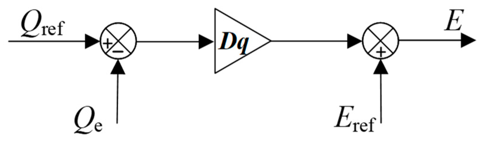
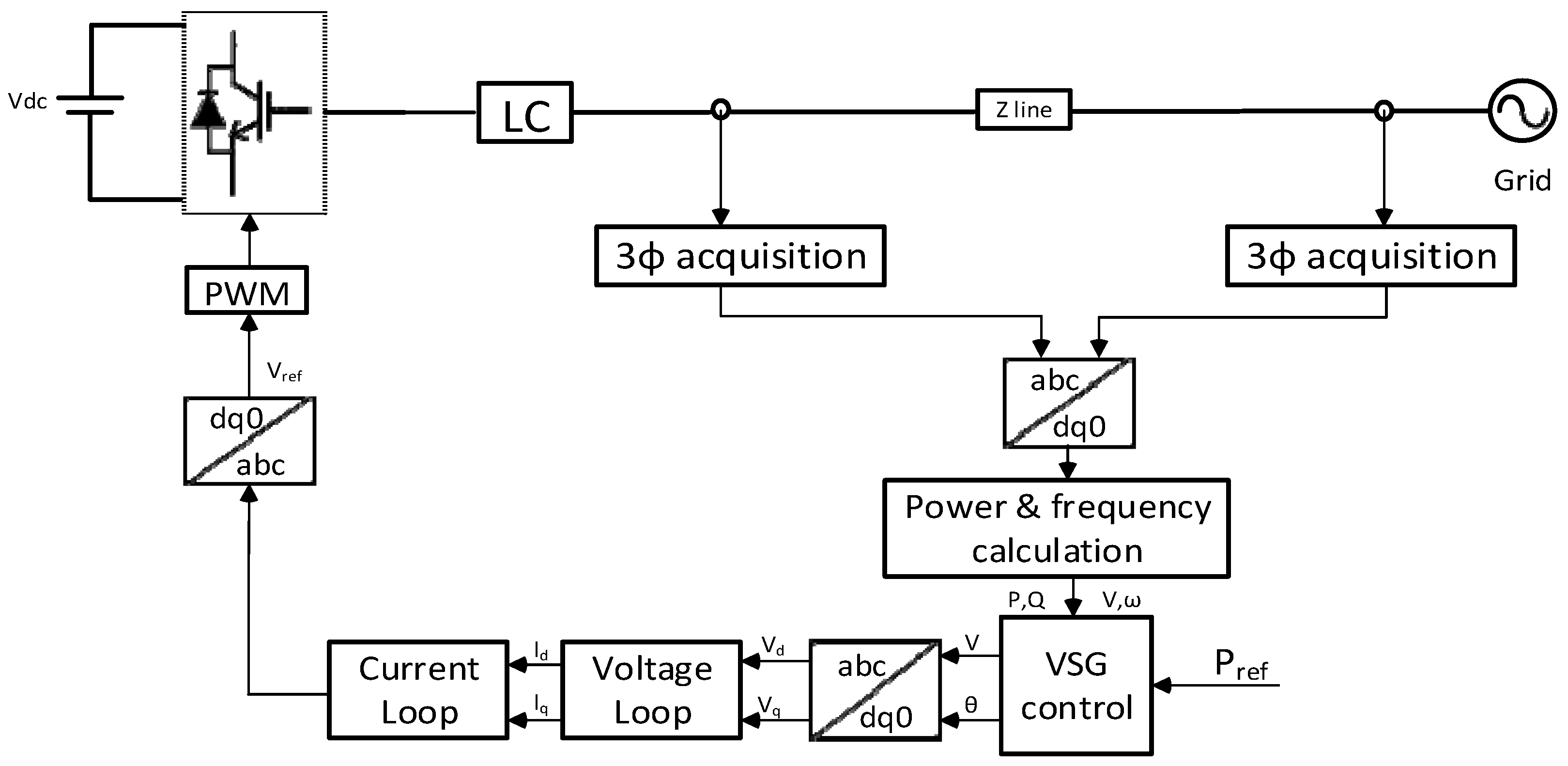
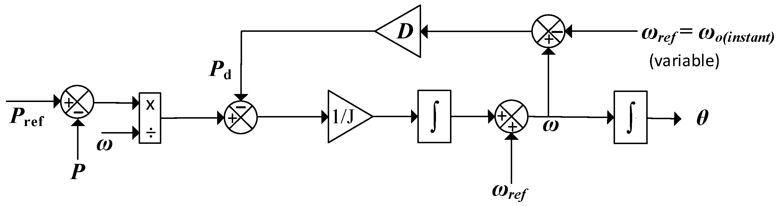
2. Operation of VSG
3. Effective Droop Control of Multiple-VSG System
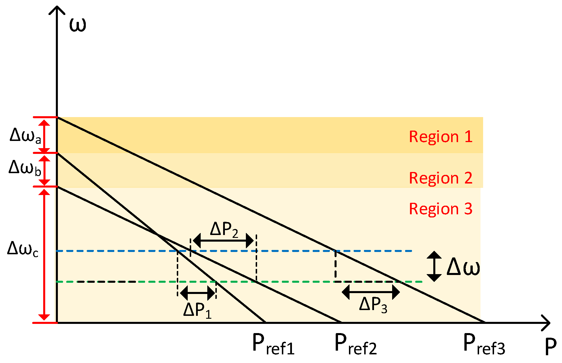
3.1. The Significance of No-Load Angular Frequency in Load Sharing
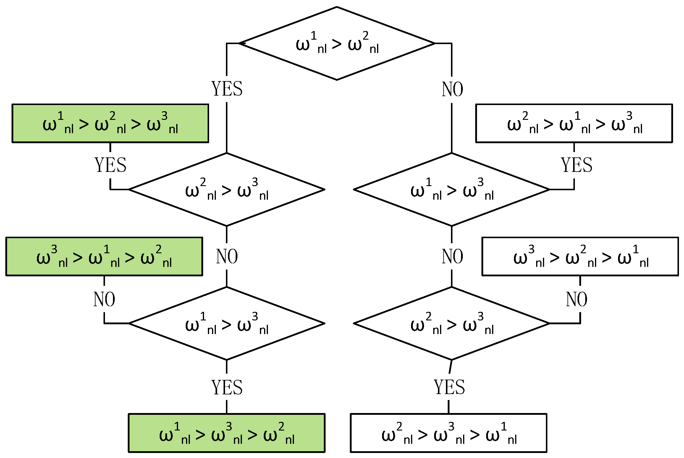
3.2. Load Sharing Criteria
3.2.1. Case I
3.2.2. Case II
3.2.3. Case III
3.3. Control for Equivalent Droop
- Case I:
- = 0.4, = 0.2, = 314.75, = 314.48, = 0.27
- Case II:
- = 0.24, = 0.16, = 314.95, = 314.53, = 0.42
- Case III:
- = 0.39, = 0.4, = 314.95, = 314.57, = 0.38
3.4. Dynamic Response of Damping Coefficient
3.5. Power Percentage
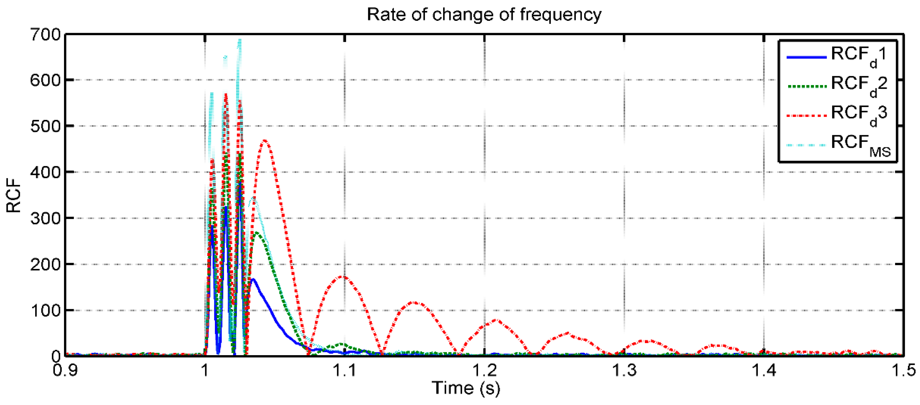
3.6. Rate of Change of Frequency (RCF)
4. Master–Slave Configuration of VSG
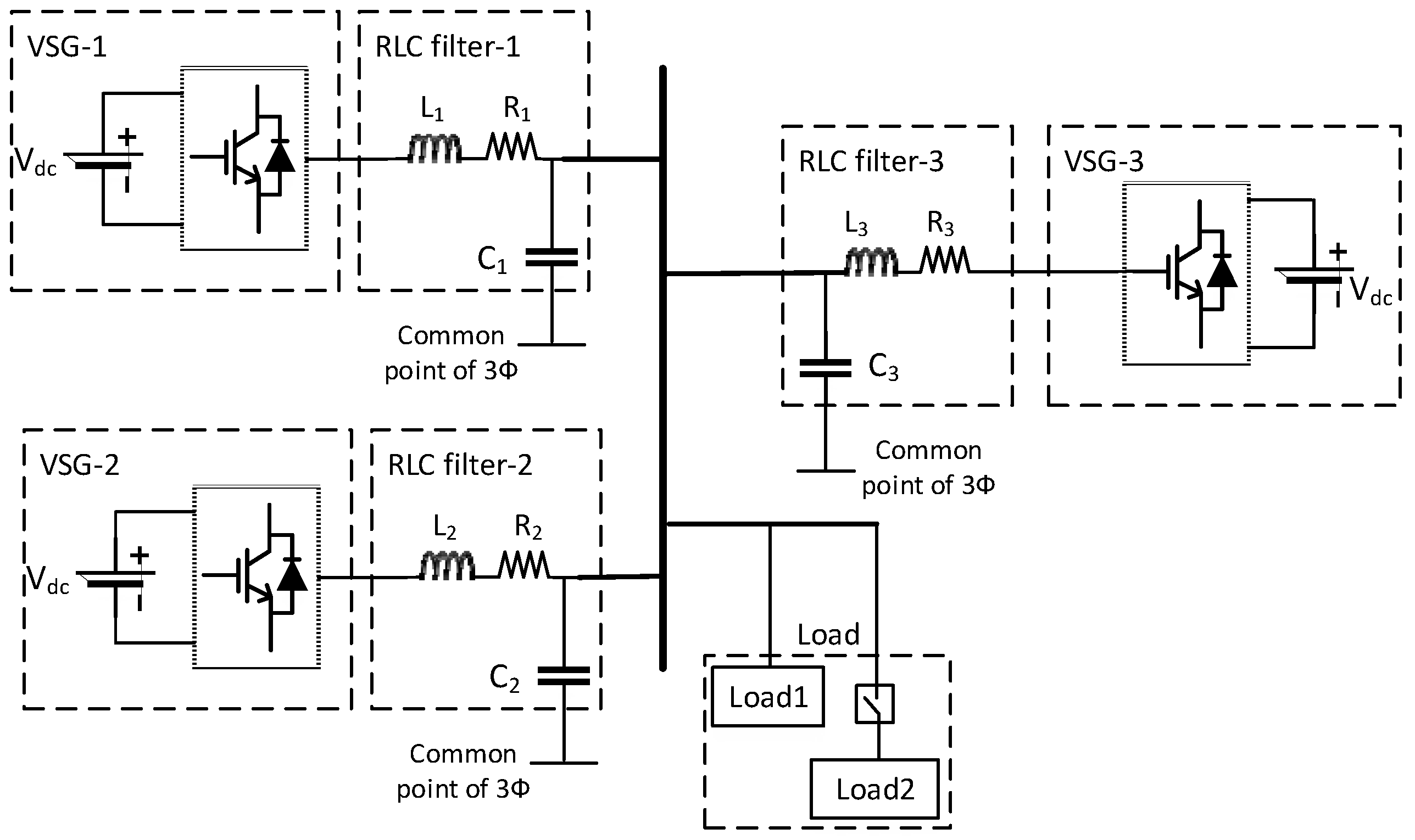
5. Island Microgrid of Multiple VSG Sources
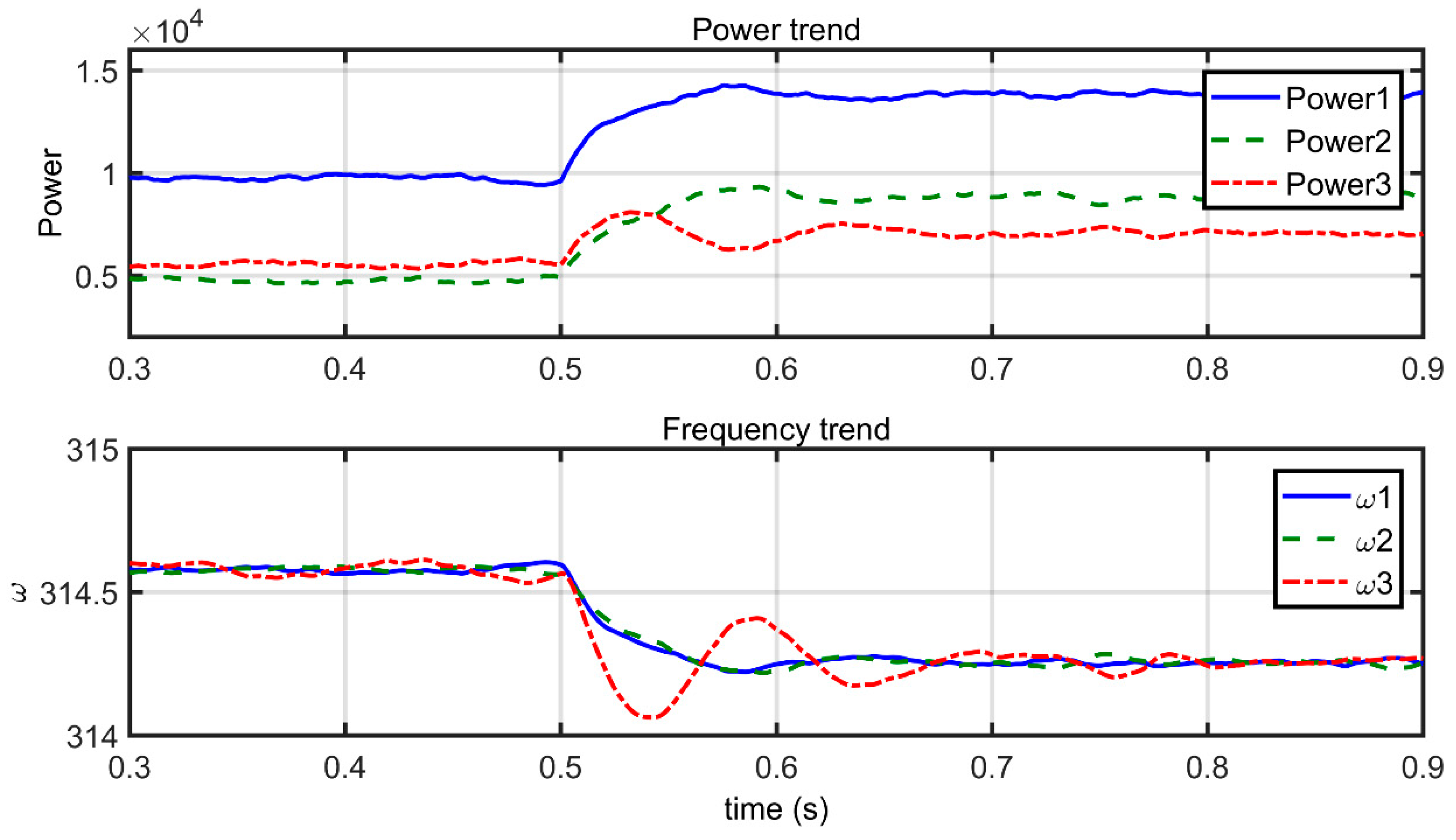
5.1. Loading Analysis
5.1.1. Case I
5.1.2. Case II
5.1.3. Case III
5.1.4. Case IV
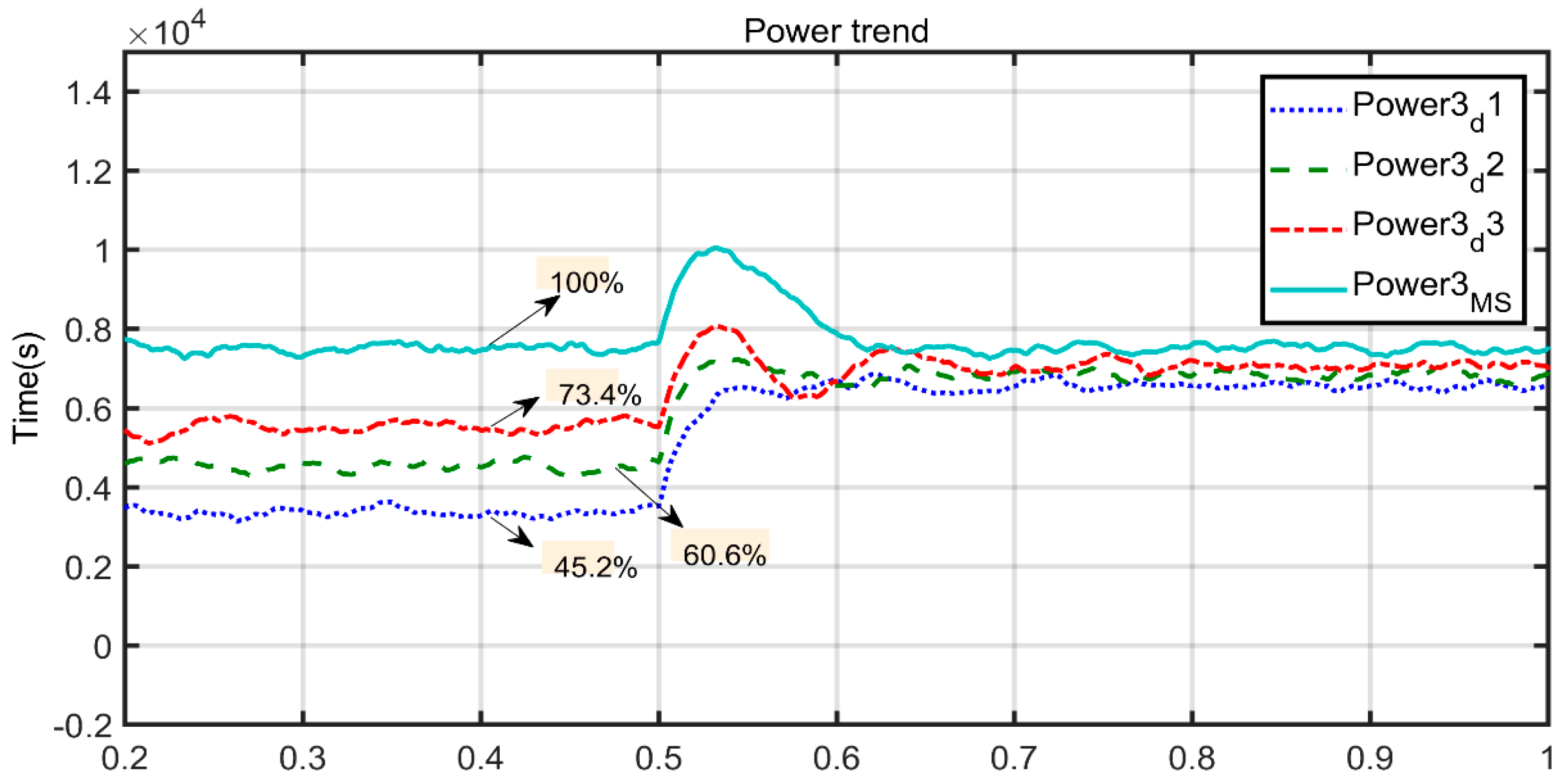
5.1.5. Comparison of Power of VSG-3
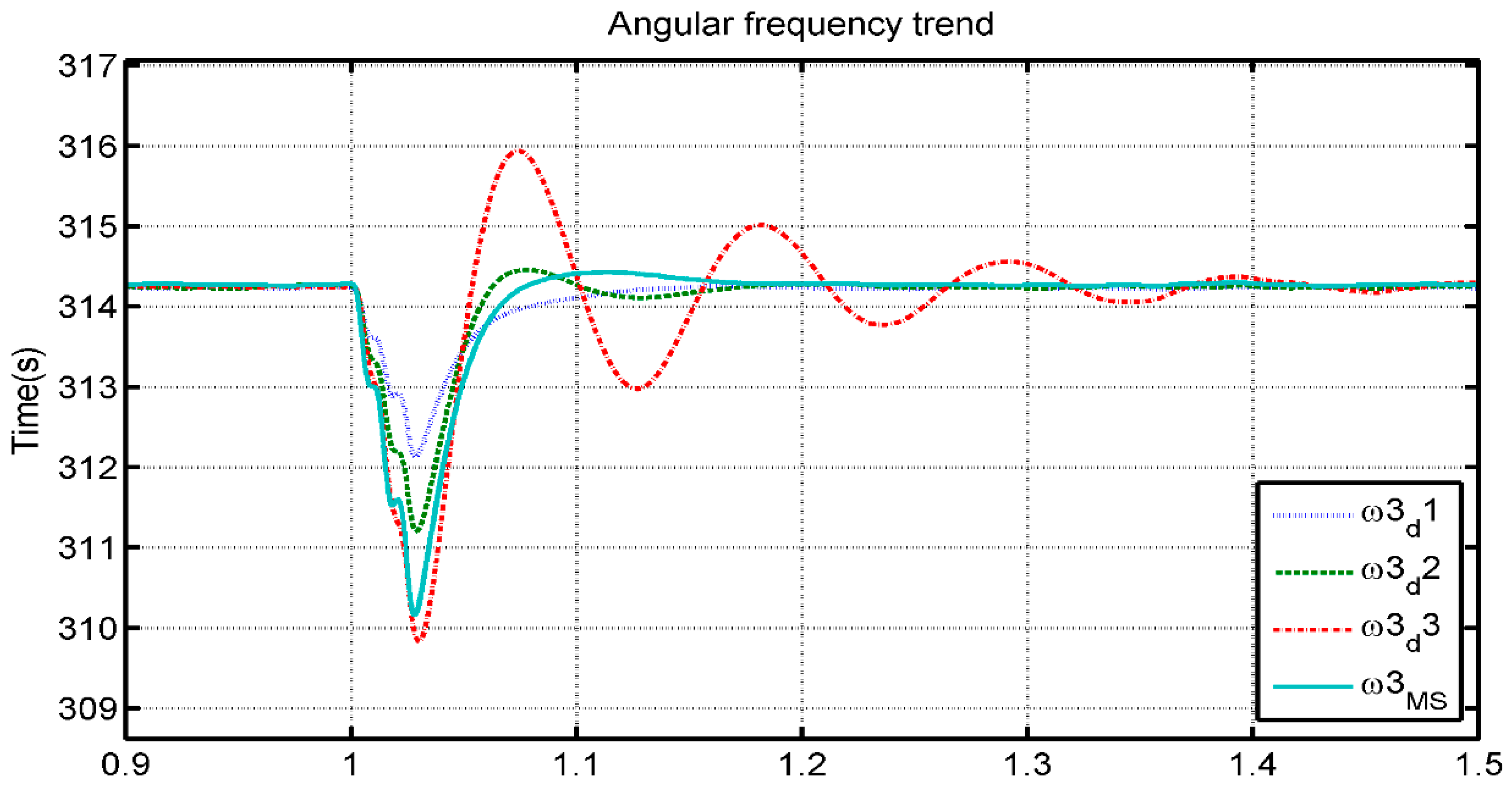
5.1.6. Comparison of Angular Frequency (VSG-3)
5.1.7. Rate of Change of Frequency Analysis
5.1.8. Comparison of RCF (VSG-3)
5.2. Fault Analysis
5.2.1. Case I
5.2.2. Case II
5.2.3. Case III
5.2.4. Case IV
5.2.5. Comparison of RCF Analysis Under Fault (VSG-3)
5.2.6. Comparison of Angular Frequency Under Fault (VSG-3)
6. Discussion
7. Conclusions
Author Contributions
Funding
Acknowledgments
Conflicts of Interest
References
- Rasool, H.; Mutal, A.; Rasool, A.; Ahmad, W.; Ikram, A.A. MPPT based ASBC controller and solar panel monitoring system. In Proceedings of the 2014 International Conference on Energy Systems and Policies (ICESP), Islamabad, Pakistan, 24–26 November 2014; IEEE: Piscataway, NJ, USA, 2014. [Google Scholar]
- Brabandere, K.D.; Bolsens, B.; Van den Keybus, J.; Woyte, A.; Driesen, J.; Belmans, R. A Voltage and Frequency Droop Control Method for Parallel Inverters. IEEE Trans. Power Electron. 2007, 22, 1107–1115. [Google Scholar] [CrossRef]
- Chandorkar, M.C.; Divan, D.M.; Adapa, R. Control of parallel connected inverters in standalone AC supply systems. IEEE Trans. Ind. Appl. 1993, 29, 136–143. [Google Scholar] [CrossRef]
- Nikkhajoei, H.; Lasseter, R.H. Distributed Generation Interface to the CERTS Microgrid. IEEE Trans. Power Deliv. 2009, 24, 1598–1608. [Google Scholar] [CrossRef]
- Vandoorn, T.L.; Meersman, B.; De Kooning, J.D.; Vandevelde, L. Analogy between conventional grid control and islanded microgrid control based on a global DC-link voltage droop. IEEE Trans. Power Deliv. 2012, 27, 1405–1414. [Google Scholar] [CrossRef]
- Hashmi, K.; Mansoor Khan, M.; Jiang, H.; Umair Shahid, M.; Habib, S.; Talib Faiz, M.; Tang, H. A Virtual Micro-Islanding-Based Control Paradigm for Renewable Microgrids. Electronics 2018, 7, 105. [Google Scholar] [CrossRef]
- Driesen, J.; Visscher, K. Virtual synchronous generators. In Proceedings of the 2008 IEEE Power and Energy Society General Meeting—Conversion and Delivery of Electrical Energy in the 21st Century, Pittsburgh, PA, USA, 20–24 July 2008. [Google Scholar]
- Hirase, Y.; Noro, O.; Yoshimura, E.; Nakagawa, H.; Sakimoto, K.; Shindo, Y. Virtual synchronous generator control with double decoupled synchronous reference frame for single-phase inverter. IEEJ J. Ind. Appl. 2015, 4, 143–151. [Google Scholar] [CrossRef]
- Chen, Y.; Hesse, R.; Turschner, D.; Beck, H.P. Improving the grid power quality using virtual synchronous machines. In Proceedings of the 2011 International Conference on Power engineering, energy and electrical drives (POWERENG), Malaga, Spain, 11–13 May 2011; IEEE: Piscataway, NJ, USA, 2011. [Google Scholar]
- Beck, H.-P.; Hesse, R. Virtual synchronous machine. In Proceedings of the 9th International Conference on Electrical Power Quality and Utilisation, EPQU 2007, Barcelona, Spain, 9–11 October 2007; IEEE: Piscataway, NJ, USA, 2007. [Google Scholar]
- Zhong, Q.-C.; Weiss, G. Synchronverters: Inverters that mimic synchronous generators. IEEE Trans. Ind. Electron. 2011, 58, 1259–1267. [Google Scholar] [CrossRef]
- Liu, J.; Miura, Y.; Bevrani, H.; Ise, T. Enhanced Virtual Synchronous Generator Control for Parallel Inverters in Microgrids. IEEE Trans. Smart Grid 2016, 8, 2268–2277. [Google Scholar] [CrossRef]
- Hirase, Y.; Noro, O.; Nakagawa, H.; Yoshimura, E.; Katsura, S.; Abe, K.; Sugimoto, K.; Sakimoto, K. Decentralised and interlink-less power interchange among residences in microgrids using virtual synchronous generator control. Appl. Energy 2018, 228, 2437–2447. [Google Scholar] [CrossRef]
- Cao, Y.; Wang, W.; Li, Y.; Tan, Y.; Chen, C.; He, L.; Häger, U.; Rehtanz, C. A Virtual Synchronous Generator Control Strategy for VSC-MTDC Systems. IEEE Trans. Energy Convers. 2018, 33, 750–761. [Google Scholar] [CrossRef]
- Wang, F.; Zhang, L.; Feng, X.; Guo, H. An Adaptive Control Strategy for Virtual Synchronous Generator. IEEE Trans. Ind. Appl. 2018, 54, 5124–5133. [Google Scholar] [CrossRef]
- Ma, Y.; Lin, Z.; Yu, R.; Zhao, S. Research on Improved VSG Control Algorithm Based on Capacity-Limited Energy Storage System. Energies 2018, 11, 677. [Google Scholar] [CrossRef]
- Alipoor, J.; Miura, Y.; Ise, T. Power System Stabilization Using Virtual Synchronous Generator With Alternating Moment of Inertia. IEEE J. Emerg. Sel. Top. Power Electron. 2015, 3, 451–458. [Google Scholar] [CrossRef]
- Shintai, T.; Miura, Y.; Ise, T. Oscillation Damping of a Distributed Generator Using a Virtual Synchronous Generator. IEEE Trans. Power Deliv. 2014, 29, 668–676. [Google Scholar] [CrossRef]
- Cheng, C.; Zeng, Z.; Yang, H.; Zhao, R. Wireless parallel control of three-phase inverters based on virtual synchronous generator theory. In Proceedings of the International Conference on Electrical Machines and Systems, Busan, South Korea, 26–29 October 2013. [Google Scholar]
- Paquette, A.D.; Reno, M.J.; Harley, R.G.; Divan, D.M. Sharing Transient Loads: Causes of Unequal Transient Load Sharing in Islanded Microgrid Operation. IEEE Ind. Appl. Mag. 2014, 20, 23–34. [Google Scholar] [CrossRef]
- Rasool, A.; Yan, X.; Rasool, H.; Guo, H.; Asif, M. VSG Stability and Coordination Enhancement under Emergency Condition. Electronics 2018, 7, 202. [Google Scholar] [CrossRef]
- Aazim, R.; Liu, C.; Haaris, R.; Mansoor, A. Rapid generation of control parameters of Multi-Infeed system through online simulation. Ingeniería e Investigación 2017, 37, 67–73. [Google Scholar] [CrossRef]
- Banu, I.V.; Istrate, M. Islanding Prevention Scheme for Grid-Connected Photovoltaic Systems in Matlab/Simulink. In Proceedings of the 2014 49th International Universities Power Engineering Conference (UPEC), Cluj-Napoca, Romania, 2–5 September 2014; IEEE: Piscataway, NJ, USA, 2014. [Google Scholar]
- Alipoor, J.; Miura, Y.; Ise, T. Stability assessment and optimization methods for microgrid with multiple VSG units. IEEE Trans. Smart Grid 2018, 9, 1462–1471. [Google Scholar] [CrossRef]
- Chen, L.; He, H.; Zhu, L.; Guo, F.; Shu, Z.; Shu, X.; Yang, J. Coordinated control of SFCL and SMES for transient performance improvement of microgrid with multiple DG units. Can. J. Electr. Comput. Eng. 2016, 39, 158–167. [Google Scholar] [CrossRef]
- Yu, B. An Improved Frequency Measurement Method from the Digital PLL Structure for Single-Phase Grid-Connected PV Applications. Electronics 2018, 7, 150. [Google Scholar] [CrossRef]


| 15 kW | 40 | 1.1936 | 315.35 |
| 10 kW | 40 | 0.7957 | 314.95 |
| 7.5 kW | 40 | 0.5968 | 314.75 |
| 7.5 kW | 25 | 0.9549 | 315.11 |
| 7.5 kW | 15 | 1.5915 | 315.74 |
| Cases | Condition | Region 1 | Region 2 | Region 3 |
|---|---|---|---|---|
| Case I | V-1 | V-1, 2 | V-1, 2, 3 | |
| Case II | V-1 | V-1, 3 | V-1, 2, 3 | |
| Case III | V-3 | V-3, 1 | V-1, 2, 3 |
| Parameter | MS–VSG (Proposed) | Simple VSG |
|---|---|---|
| Variable frequency | Fixed frequency | |
| Inertia | Yes | Yes |
| Damping | Yes | Yes |
| Power deliver | Ref. power at any ω | Ref. power at ωref (100π) |
| droop | Only Dynamic state | Both Static and Dynamic state |
| droop | Yes | Yes |
| Dependency of factor ‘D’ | Damping | Droop and damping both |
| Para. | Values | Para. | Values | Para. | Value |
|---|---|---|---|---|---|
| P1 | 15 kW | P2 | 10 kW | P3 | 7.5 kW |
| Vref | 380 V | Vref | 380 V | Vref | 380 V |
| ω | 2π × 50 | fpwm | 5000 Hz | fpwm | 5000 Hz |
| fn | 50 Hz | fn | 50 Hz | fn | 50 Hz |
| D(VSG-1) | 40 | D(VSG-2) | 40 | D(VSG-3) | 40, 25, 15 |
| R1 | 0.05 | R2 | 0.05 | R3 | 0.05 |
| L1 | 1.45 × 10⁻³ | L2 | 1.45 × 10⁻³ | L3 | 1.45 × 10⁻³ |
| C1 | 150 × 10−6 | C2 | 150 × 10−6 | C3 | 150 × 10−6 |
| Vdc | 800 V | Vdc | 800 V | Vdc | 800 V |
| Dq1 | 0.010 | Dq2 | 0.010 | Dq3 | 0.010 |
| J1 | 0.1 | J2 | 0.1 | J3 | 0.1 |
| Cases | Condition | ||||||||||
|---|---|---|---|---|---|---|---|---|---|---|---|
| Case I | 0.4 | 0.2 | 0.27 | 314.48 | 10.9 | 5.9 | 3.39 | 72.8 | 59 | 72.8 | |
| Case II | 0.24 | 0.16 | 0.42 | 314.53 | 10.3 | 5.27 | 4.55 | 68.7 | 52.7 | 68.7 | |
| Case III | 0.39 | 0.4 | 0.38 | 314.57 | 9.8 | 4.77 | 5.57 | 65.34 | 47.4 | 65.3 | |
| Case IV | 0.4 | - | - | 314.65 | 8.75 | 3.75 | 7.5 | 58.3 | 37.5 | 100 |
© 2018 by the authors. Licensee MDPI, Basel, Switzerland. This article is an open access article distributed under the terms and conditions of the Creative Commons Attribution (CC BY) license (http://creativecommons.org/licenses/by/4.0/).
Share and Cite
Yan, X.; Rasool, A.; Abbas, F.; Rasool, H.; Guo, H. Analysis and Optimization of the Coordinated Multi-VSG Sources. Electronics 2019, 8, 28. https://doi.org/10.3390/electronics8010028
Yan X, Rasool A, Abbas F, Rasool H, Guo H. Analysis and Optimization of the Coordinated Multi-VSG Sources. Electronics. 2019; 8(1):28. https://doi.org/10.3390/electronics8010028
Chicago/Turabian StyleYan, Xiangwu, Aazim Rasool, Farukh Abbas, Haaris Rasool, and Hongxia Guo. 2019. "Analysis and Optimization of the Coordinated Multi-VSG Sources" Electronics 8, no. 1: 28. https://doi.org/10.3390/electronics8010028
APA StyleYan, X., Rasool, A., Abbas, F., Rasool, H., & Guo, H. (2019). Analysis and Optimization of the Coordinated Multi-VSG Sources. Electronics, 8(1), 28. https://doi.org/10.3390/electronics8010028