Article

An Event-Triggered Fault Detection Approach in Cyber-Physical Systems with Sensor Nonlinearities and Deception Attacks

Engineering Research Center of Internet of Things Technology Applications (Ministry of Education), Jiangnan University, Wuxi 214122, China
*
Author to whom correspondence should be addressed.
Electronics 2018, 7(9), 168; https://doi.org/10.3390/electronics7090168
Submission received: 4 August 2018 / Revised: 22 August 2018 / Accepted: 27 August 2018 / Published: 30 August 2018
(This article belongs to the Special Issue Recent Developments on Time-Delay Systems and Its Applications)

Abstract

:
In this paper, a general event-triggered framework is constructed to investigate the problem of remote fault detection for stochastic cyber-physical systems subject to the additive disturbances, sensor nonlinearities and deception attacks. Both fault-detection residual generation and evaluation module are fully described. Two energy norm indices are presented so that the fault-detection residual has the best sensitivity to faults and the best robustness to unwanted factors including additive disturbances and false information injected by attacker. Moreover, the filter gain and residual weighting matrix are formulated in terms of stochastic Lyapunov function, which can be conveniently solved via standard numerical software. Finally, an application example is presented to verify the performance of fault detection by comparative simulations. The prolonged battery life is experimentally evaluated and analyzed via a wireless node platform.

1. Introduction

Cyber-Physical Systems (CPSs) refer to the integration of sensing, control, communication, computation and physical processes [1]. These tightly integrated systems extend existing networked systems (such as networked control systems (NCSs) [2] and wireless sensor networks (WSNs) [3]) in both size and complexity. Applications of CPSs are promising in areas including smart grid [4], autonomous automobile systems [5], medical monitoring and process control systems [6]. Their reliability and stability, however, are very susceptible to operational and environmental conditions [7]. This is why a health management unit for CPSs should be established for health monitoring and diagnosis. The reliability problems are not new in the NCSs field, in particular in the areas of model-based fault diagnosis approach [8,9,10]. In the model-based fault-detection approach, state observers or filters are usually used to generate residual signals, which are smaller than pre-designated thresholds when no faults exist [11].
In WSNs, information transmission from sensor to a remote estimator/actuator consumes energy that is often a significant fraction of the system’s overall energy balance. Similar to the WSNs, communication resources for CPSs are also limited. Recently, an event-triggered transmission scheme has received a lot of attention to overcome the limitations of traditional design methodologies for resource-constrained problems [12,13,14,15]. Summarizing the existing works, we can easily find that data are transmitted or processed only when certain events indicate that an update is required. Hence, resources can be used only when require and saved otherwise. Another issue which should be considered is related to deception attacks in data transmission. This kind of attack may be imposed because of the pervasive utilization of shared yet unprotected communication channels. In addition, it is well known that wireless sensors are often placed in harsh environment; thus, various environmental cases can influence various aspects of sensor performance, which may lead to a nonlinear characteristic of sensor [16]. Before addressing the main contribution of this paper, we briefly review some related literature.

1.1. Related Work

Event-triggered transmission scheme, which can reduce the network utilization, has been widely used for a variety of systems (e.g., [17,18,19,20,21]). An output estimation error-based scheme with a switching Kalman filter is proposed in [22] as a new framework for event-triggered state estimation. Two different event conditions for fault-tolerant control are studied in [23] in terms of the system state and the system state error, respectively. A great deal of research progress has been made (see [24,25,26,27,28,29,30] and the references therein). It was shown in [31] that the deception attacks are viewed as the most dangerous attack behaviors and, therefore, some solutions against deception attacks have been proposed. For example, a security-guaranteed filtering problem in [31] is studied, where a new security criterion is introduced including the noise intensity, the energy bound of the false signals, the energy of the initial system state, and the desired security degree. In [32], a coordinate transformation approach is exploited for a synthesized design of fault-detection filter and fault estimator against false data injection attacks. A jamming attack issue is considered in [33] for remote state estimation of CPSs, where the sensor and the attacker with constrained resources are regarded as the two players of a zero-sum game. It follows from the existing literature that the problem of event-triggered fault detection for CPSs subject to deception attacks is of significant importance. If the sensor nonlinearities are ignored during the system design process, undesirable performance may occur and even deteriorate the system stability. Some representative results have been proposed to address this problem involving Lipschitz conditions, sector-bounded conditions and immersion conditions (see [34,35,36] and the references therein).

1.2. Main Contribution

However, most existing results only take the secure estimation/control problem into account, and secure fault-detection filter design for CPSs still remains open and challenging. Especially, the main motivation of this paper is how to defend the effects of the deception attacks, sensor nonlinearities and additive disturbances under the event-triggered decision rule. Moreover, while most of the previous results are proposed for deterministic systems, providing an effective method for stochastic systems also motivates the present study. The main contribution of this paper includes three aspects:
(1)
A new event-triggered fault-detection filter for CPSs is proposed against the phenomena of sensor nonlinearities, deception attacks and additive disturbances, where the sensor nonlinearities is assumed to occur randomly according to a random variable satisfying the Bernoulli distribution.
(2)
A fault-detection filter problem is formulated by maximizing the sensitivity of faults and minimizing the influences of additive disturbances and false information injected by attackers. The filter gain and residual weighting matrix are derived by stochastic Lyapunov function, which can be easily solved via standard numerical software.
(3)
At the end of this paper, an application example to event-triggered fault detection of one-dimensional target tracking is presented. The estimation accuracy and fault-detection capacity are demonstrated by comparative simulations. The prolonged battery life is experimentally evaluated and analyzed via a wireless node platform.
Nomenclature: The terms filter and state estimator are used synonymously in this paper. N and R denote the sets of natural and real numbers, respectively. R m × n denotes the sets of m by n real-valued matrices, whereas R n is short for R n × 1 . R + n × n and R + + n × n are the sets of n × n positive semi-definite and positive definite matrices, respectively. When X R + n × n , it is simply denoted as X 0 or X > 0 if X R + + n × n . For X R m × n , X T denotes the transpose of X. A diagonal matrix is denoted by d i a g · . In symmetric block matrices, “*” is used as an ellipsis for terms induced by symmetry. I denotes a identity matrix with appropriate dimensions. λ min X and λ max X are minimum and maximum eigenvalues of matrix X, respectively. Furthermore, a diagonal matrix is denoted by d i a g · , and 2 0 , is the space of square integrable vectors. E [ · ] and Prob x denote the mathematical expectation and the occurrence probability of the event x, respectively.

2. Problem Statement

Consider the following discrete-time stochastic CPS defined on a probability space ( Ω , F , P )
x k + 1 = A 1 x k + A 2 x k + D 1 d k w k + F 1 f k
where the (unavailable) system state vectors , the unknown disturbances and fault signals represent x k R n , d k R q and f k R r , respectively. A scalar Wiener process w k is defined on a complete space ( Ω , F , P ) with E w k = 0 , E w k 2 = 1 and E w i w j = 0 ( i j ), where Ω is the sample space, F is the σ -algebra of subsets of the sample space, and P is the probability measure on F . Fault and disturbance signals are assumed to be 2 signals ( f , w 2 s ).
The measurement model with randomly occurring sensor nonlinearities is described by
y ¯ k = 1 β k s C ¯ x k + β k C ¯ x k + D 2 d k + F 2 f k y k = y ¯ k + M y a , k y a , k = y ¯ k + ε k
In the above sensor model, y ¯ k are ideal measurement values, and y ¯ k R s are measurement values subject to randomly occurring sensor nonlinearities, which are satisfied with the following condition:
s η S 1 η T s η S 2 η 0
In Equation (3), S 2 > S 1 > 0 and η R s are two diagonal matrices and a scalar, respectively. The random constant variable is a Bernoulli-distributed white sequence which can be described as follows
Prob β k = 1 = β a n d Prob β k = 0 = 1 β
for a given positive scalar β 0 , 1 . Furthermore, the matrices A 1 , A 2 , A d , D 1 , F 1 , C ¯ , D 2 and F 2 are known constant matrices with appropriate dimensions. The random variable β k is uncorrelated with noise process w k .
Remark 1.
Many actual applications inevitably result in the sensor saturations which have the nonlinear characteristic of sensors. This characteristic can severely restrict system performance or, even worse, lead to undesirable oscillatory behaviors [37]. Recently, the design of reliable controller and estimator against sensor saturations for various systems has received increasing attention [37,38,39]. Note that all the above works are based on a common assumption that the sensor saturation occurs persistently. However, the sensor saturation itself may be subject to randomly fluctuated condition changes because it can be considered in a network environment. Hence, this assumption has been removed in this paper. In addition, since the randomly occurring sensor saturation is taken into account in event-triggered fault-detection filter design, the result obtained is less conservative.
As discussed in Section 1, the information sent by attackers during the network transmission is modeled as follows
y a , k = M y ¯ k + M ε k
where the information y a , k is used by the adversary for the deception attacks, and the non-zero ε k 2 , is an unknown but energy-bounded information. The matrix M represents the physical constraints of attack information, and is assumed to be of the following form
M ̲ M M ¯
where the unknown but bounded matrix M has an upper bound M ¯ > 0 and a lower bound M ̲ > 0 .
Remark 2.
It should be mentioned that, from the adversary’s perspective, the unknown but bounded matrix M is regarded as physical constraints in the model of deception attacks (Equation (5)) which was introduced in [40]. Such physical constraints are unavoidable such as launching devices powered by limited capacity, networks with limited bandwidth, and defender’s system equipped with protection software [41]. Hence, the established attack model in Equation (5) under consideration is quite comprehensive that is closer to the practical engineering case. On the other hand, the sensitivity problem of fault-detection becomes more complicated because the false information ε k sent by attacker is assumed to be energy-bounded, which has a similar form as additive disturbances and system faults.
For technical convenience, the actual measurement can be decomposed into a linear and a nonlinear part as
y k = y ¯ k + M ̲ y a , k + ϕ y a , k
where
ϕ T y a , k ϕ y a , k M ˜ y a , k 0
and a positive definite matrix M ˜ = Δ M ¯ M ̲ .
The introduction of the stochastic variables w k and β k render the fault-detection filter to be stochastic instead of a deterministic one. Thus, before proceeding further, it is necessary to introduce the notion of stability in the mean-square sense.
Definition 1.
A discrete stochastic process ξ k is said to be mean-square stable, if there exist constants ρ ˜ 1 0 , ρ ˜ 2 > 0 and 0 ρ ˜ 3 < 1 such that
E ξ k 2 ρ ˜ 1 + ρ ˜ 2 1 ρ ˜ 3 k , k I +
where I + is the set of positive integer.
Traditionally, the system stability is studied by using the Lyapunov’s methodology. The following lemma presents sufficient conditions for the mean-square stability of a stochastic system in terms of a stochastic Lyapunov functional.
Lemma 1.
[10] Let V ρ k be a Lyapunov functional. If there exist real scalars ρ 1 0 , ρ 2 > 0 , ρ 3 > 0 and 0 < ρ 4 1 such that
ρ 2 ρ k 2 V ρ k ρ 3 ρ k 2
and
E V ρ k + 1 ρ k V ρ k ρ 1 ρ 4 V ρ k
then the sequence ρ k satisfies
E ρ k 2 ρ 3 ρ 2 ρ 0 2 1 ρ 4 k + ρ 1 ρ 2 ρ 4
Remark 3.
It can be noted that if the conditions in Equations (10) and (11) hold, it follows easily from ρ ˜ 1 = ρ 1 ρ 2 ρ 4 , ρ ˜ 2 = ρ 3 ρ 2 ρ 0 2 and Definition 1 that the stochastic process ρ k is mean-square stable.

3. Event-Triggered Fault-Detection Filter Analysis and Design

Generally speaking, fault detection mainly contains a residual generator and a residual evaluator as in [11]. The event-triggered fault-detection filter is presented and its mean-square stability is proved.

3.1. Residual Generator

For the purpose of residual generation, the following fault-detection filter is constructed:
x ^ k + 1 = A 1 x ^ k + L y i k y ^ k y ^ k = β C x ^ k
where x ^ k is the estimated system state, L is a filter gain with appropriate dimensions to be determined, y ^ k denotes output estimation information and C = I M ̲ C ¯ . To save computation and communication resources, an event-triggered sensor data transmission scheme is introduced to determine whether the measurement information should be transmitted. The variables i k and y i k denote the last released instant and the released measurement information, respectively, with  k i k , i k + 1 , and i k + 1 is the next released instant of the event generator.
The error state e k , the output estimation error e y , k and the residual signal r k are defined as the following form
e k = x k x ^ k e y , k = y i k y ^ k r k = V y i k y ^ k
where V is a residual weighting matrix to be designed. Subtracting estimator Equation (13) from system Equation (1) results in the following estimation error dynamics
e k + 1 = x k + 1 x ^ k + 1 = A 1 e k + A 2 x k + D 1 d k w k + F 1 f k L y k y ^ k = A 1 β L C e k + F 1 L M ^ F 2 f k M ^ 1 d ˜ k L ϕ y a , k L Ξ k β 1 L M ^ s C ¯ x k β k β L C x k + β k β L M ^ s C ¯ x k + A 2 x k + D 1 d k w k
where y ^ k = β C x ^ k , d ˜ k = d k T , ε k T T , M ^ 1 = L M ^ D 2 , L M ̲ , β 1 = 1 β , M ^ = I M ̲ and Ξ k = y i k y k .
The purpose of this section is that the designed fault-detection filter (Equation (13)) should be robust against randomly occurring sensor nonlinearities and deception attacks. More specifically, we are interested in looking for the filter gain L and the residual weighting matrix V such that the following requirements are met simultaneously:
(1)
The dynamic error system in Equation (15) is mean-square stable when d ˜ k = 0 or f k = 0 .
(2)
Under the zero initial condition, the fault-detection filter satisfies
E r k T r k < γ 1 2 E d ˜ k T d ˜ k
E r k T r k > γ 2 2 E f k T f k
for all admissible d k , ε k and f k .
Remark 4.
Requirement (1) ensures mean-square stability of estimation error e k . Requirement (2) on the high sensitivity to the faults and simultaneously the strong robustness to the additive disturbances d k and false information ε k sent by attacker is, in fact, a multiple-objective optimization problem that can be formulated as finding a fault-detection filter (Equation (13)) to minimize γ 1 and maximize γ 2 .
In the following, robustness against additive disturbances d k and malicious data ε k is studied. To achieve this objective, a fault-detection filter with the fault-free case ( f k = 0 ) is designed such that E r k T r k < γ 1 2 E d ˜ k T d ˜ k , where γ 1 measures the disturbances robustness in the fault-free case.
Theorem 1.
Consider the system in Equation (1) in the fault-free case f k = 0 with the sensor measurements in Equation (7) subject to randomly occurring sensor nonlinearities and deception attacks. For given γ 1 > 0 , if there exists positive definite symmetric matrices P j j = 1 a n d 2 , two real scalars λ 1 and λ 2 as well as matrix R with appropriate dimensions such that the following LMI is satisfied
Λ = Λ ˜ 11 Λ ˜ 12 Λ ˜ 12 T Λ ˜ 22 Λ ˜ 2 Λ ˜ 3 1 Λ ˜ 2 T < 0
where
Λ ˜ 11 = P 1 0 0 0 λ 1 2 I 0 0 * γ 1 2 I 0 . 5 M ˜ T * * I
Λ ˜ 12 = 0 0 0 0 0 0 0 0 0 0 . 5 β 1 M ˜ 0 . 5 β M ˜ C ¯ 0 . 5 M ˜ D 2
Λ ˜ 22 = Λ ^ 1 T Λ ^ 2 T T Λ ^ 1 = I 0 . 5 S 2 C ¯ + S 1 C ¯ 0 Λ ^ 11 A 2 T P 1 + P 2 D 1 Λ ^ 11 = A 2 T P 1 A 2 C ¯ T S 1 T S 2 C ¯ Λ ^ 2 = * * 0 * D 1 T P 1 + P 2 D 1 γ 1 2 I Λ ˜ 2 = Λ ¯ 2 T Λ ¯ 3 T Λ ¯ 4 T Λ ¯ 5 T T Λ ¯ 2 = A 1 T P 1 T β C T R T 0 0 β C T V T 0 0 0 R T 0 0 V T 0 0 0 Λ ¯ 3 = M ̲ T R T 0 0 M ̲ T V T 0 M ̲ T 0 R T 0 0 V T 0 I 0
Λ ¯ 4 = β 1 M ^ T R T M ^ T R T 0 β 1 M ^ T V T 0 C T R T A 1 T P 0 M ^ T V T β 1 M ^ T M ^ T C T V T 0 C T Λ ¯ 5 = D 2 T M ^ T R T 0 0 D 2 T M ^ T V T 0 D 2 T M ^ T 0
and
Λ ˜ 3 = d i a g P 1 , β 2 1 P 1 , P 2 , I , β 2 1 I , λ 2 1 I , λ 2 1 β 2 1 I
with β 1 = 1 β , M ^ = I M ̲ , C = I M ̲ C ¯ and β 2 = E β k β 2 = β β 2 , then the estimation error in Equation (15) is mean-square stable when d ˜ k = 0 under the event condition
λ 1 Ξ k T Ξ k λ 2 y k β C x ^ k T y k β C x ^ k
In addition, the residual r k satisfies E r k 2 < γ 1 2 E d ˜ k 2 , where d ˜ k = d k T , ε k T T . The filter gain can be computed by L = P 1 1 R .
Proof. 
The proof is given in Appendix A.  □
Remark 5.
If Ξ k = 0 , then it is easily checked that y i k = y k . This means that the presented event-triggered fault-detection filter will reduce to a traditional time-driven H filter [42]. Therefore, according to Theorem 1, the following corollary can extend to the case of time-driven fault-detection filter.
Corollary 1.
Assume that Ξ k = 0 . Consider that Theorem 1 holds. For given γ 1 > 0 , if there exists positive definite symmetric matrices P j j = 1 a n d 2 and matrix R with appropriate dimensions such that the condition in Equation (18) is satisfied, then the filter in Equation (13) is reduced to time-driven H filter and the estimation error in Equation (15) is mean-square stable when d ˜ k = 0 . In addition, the residual r k satisfies E r k 2 < γ 1 2 E d ˜ k 2 , where d ˜ k = d k T , ε k T T . The filter gain can be computed by L = P 1 1 R .
Proof. 
The derivation of Corollary 1 is similar to that of Theorem 1; it is therefore omitted. □
In the following, the sensitivity problem of the residual r k to fault f k is considered. To achieve this goal, a fault-detection filter with the disturbance-free case d ˜ k = 0 will be designed such that E r k 2 > γ 2 2 E f k 2 , where γ 2 measures the fault sensitivity in the disturbance-free case.
Theorem 2.
Consider stochastic system described by Equation (1) in the presence of disturbance-free case ( d ˜ k = 0 ) and the measurements in Equation (2) suffering from randomly occurring sensor nonlinearities and deception attacks. For a given positive scalar γ 2 , if there exist positive definite symmetric matrices P j j = 5 a n d 6 , two real scalars λ 1 and λ 2 as well as matrix R ¯ with appropriate dimensions, such that the following LMI is satisfied
Θ = Θ ˜ 11 Θ ˜ 12 Θ ˜ 12 T Θ ˜ 22 Θ ˜ 2 Θ ˜ 3 1 Θ ˜ 2 T < 0
where
Θ ˜ 11 = P 5 0 0 0 λ 1 2 I 0 0 0 I
Θ ˜ 12 = 0 0 0 0 0 0 0 . 5 β 1 M ˜ 0 . 5 β M ˜ C ¯ 0 . 5 M ˜ F 2
Θ ˜ 22 = I 0 . 5 S 2 C ¯ + S 1 C ¯ 0 Θ ^ 22 0 * γ 2 2 I Θ ^ 22 = A 2 T P 5 + P 6 A 2 P 6 C ¯ T S 1 T S 2 C ¯
Θ ˜ 2 = Θ ¯ 1 T Θ ¯ 2 T Θ ¯ 3 T T Θ ¯ 1 = Θ ¯ 11 0 0 β C T V T 0 β C T 0 R ¯ T 0 0 0 0 0 0 Θ ¯ 11 = A 1 T P 5 T β C T R ¯ T Θ ¯ 2 = R ¯ T 0 0 V T 0 I 0 Θ ¯ 22 Θ ¯ 66 0 Θ ¯ 33 Θ ¯ 44 Θ ¯ 55 M ^ T Θ ¯ 22 = β 1 M ^ T R ¯ T , Θ ¯ 33 = β 1 M ^ T V T , Θ ¯ 44 = M ^ T V T Θ ¯ 55 = β 1 M ^ T , Θ ¯ 66 = M ^ T R T
Θ ¯ 3 = 0 C T R T A 1 T P 6 0 C T V T 0 C T Θ ¯ 77 0 F 1 T P 6 Θ ¯ 88 0 Θ ¯ 99 0 Θ ¯ 77 = F 1 T P 5 T F 2 T M ^ T R ¯ T , Θ ¯ 88 = F 2 T M ^ T V T , Θ ¯ 99 = F 2 T M ^ T
and
Θ ˜ 3 = d i a g P 5 , β 2 1 P 5 , P 6 , I , β 2 1 I , λ 2 1 I , λ 2 1 β 2 1 I
with β 1 = 1 β , M ^ = I M ̲ , C = I M ̲ C ¯ and β 2 = E β k β 2 = β β 2 , then the estimation error in Equation (15) is exponentially mean-square stable when f k = 0 , and guarantees that E r k 2 > γ 2 2 E f k 2 . Moreover, the event condition in Equation (23) is satisfied and the filter gain can be computed by L = P 5 1 R ¯ .
Proof. 
The proof is presented in Appendix B. □
Similar to Corollary 1, The results proposed in Theorem 2 are extended to the case of time-driven fault-detection filter, as claimed by the following corollary.
Corollary 2.
Assume that Ξ k = 0 . Consider that Theorem 2 holds. For given γ 2 > 0 , if there exists positive definite symmetric matrices P j j = 5 a n d 6 and matrix R ¯ with appropriate dimensions such that the condition in Equation (24) is satisfied, then the filter in Equation (13) is reduced to time-driven H filter and the estimation error in Equation (15) is mean-square stable when f k = 0 . In addition, the residual r k satisfies E r k 2 > γ 2 2 E f k 2 . The filter gain can be computed by L = P 5 1 R ¯ .
Proof. 
The derivation of Corollary 2 is similar to that of Theorem 2; it is therefore omitted. □
Remark 6.
Theorem 1 provides the worst-case criterion for the effects of additive disturbances and false information sent by attacker on the residual. Satisfaction of the performance index in Equation (16) ensures that the filter gain from d ˜ k to e k is less than γ 1 2 . On the other hand, Theorem 2 obtains the sensitivity of the residual to system faults. Satisfaction of the performance index in Equation (17) ensures that the filter gain from f k to e k is more than γ 2 2 . Both give a directly quantitative indicator for robustness and sensitivity of event-triggered fault-detection filter.
Inspired by [42], the following algorithm 1 is utilized to compute the filter parameters so as to achieve the optimal trade-off between robustness against d ˜ k and sensitivity to f k .
Algorithm 1 Computation of event-triggered fault-detection filter parameters
Step 1: Calculate the minimum of γ 1 and the maximum of γ 2 using Equations (18) and (24) in Theorem 1 and Theorem 2, respectively.
Step 2: Replace the minimum of γ 1 in Equation (18) and the maximum of γ 2 in Equation (24) with γ 1 and γ 2 , respectively.
Step 3: If the obtained γ 1 and γ 2 can make Equations (18) and (24) feasible simultaneously, then the optimal filter gain L and the residual weighting matrix V can be determined. Otherwise, go to Step 3.
Step 4: Choose a sufficient positive constant Δ γ . Assign γ 1 = γ 1 + Δ γ and γ 2 = γ 2 Δ γ . Solve Equations (18) and (24) with the updated γ 1 and γ 2 .
Step 5: Repeat Steps 2–4 until the conditions in Equations (18) and (24) are feasible.
Step 6: Construct the residual generator r k in Equation (14), and the filter in Equation (13).
End

3.2. Residual Evaluator

As mentioned in Section 3.1, the responsibility of the residual evaluation is to produce appropriate fault alarms. The prescribed evaluation function is compared with the predefined threshold J t h . If the value of the evaluation function exceeds J t h , an alarm of fault is triggered. We choose
r T = 1 T k = t 0 t 0 + T 1 r k T r k
as the residual evaluation function, where t 0 denotes the initial evaluation time instant and T stands for the evaluation time. It should be noted that the evaluation time T is limited because the evaluation of residual signal over the whole time horizon is impractical. Let J t h = Δ sup d ˜ k 2 , f k = 0 r T be the threshold. For a given threshold J t h , the generation of the alarms can be outlined in Algorithm 2.
Algorithm 2 Fault-alarming strategy
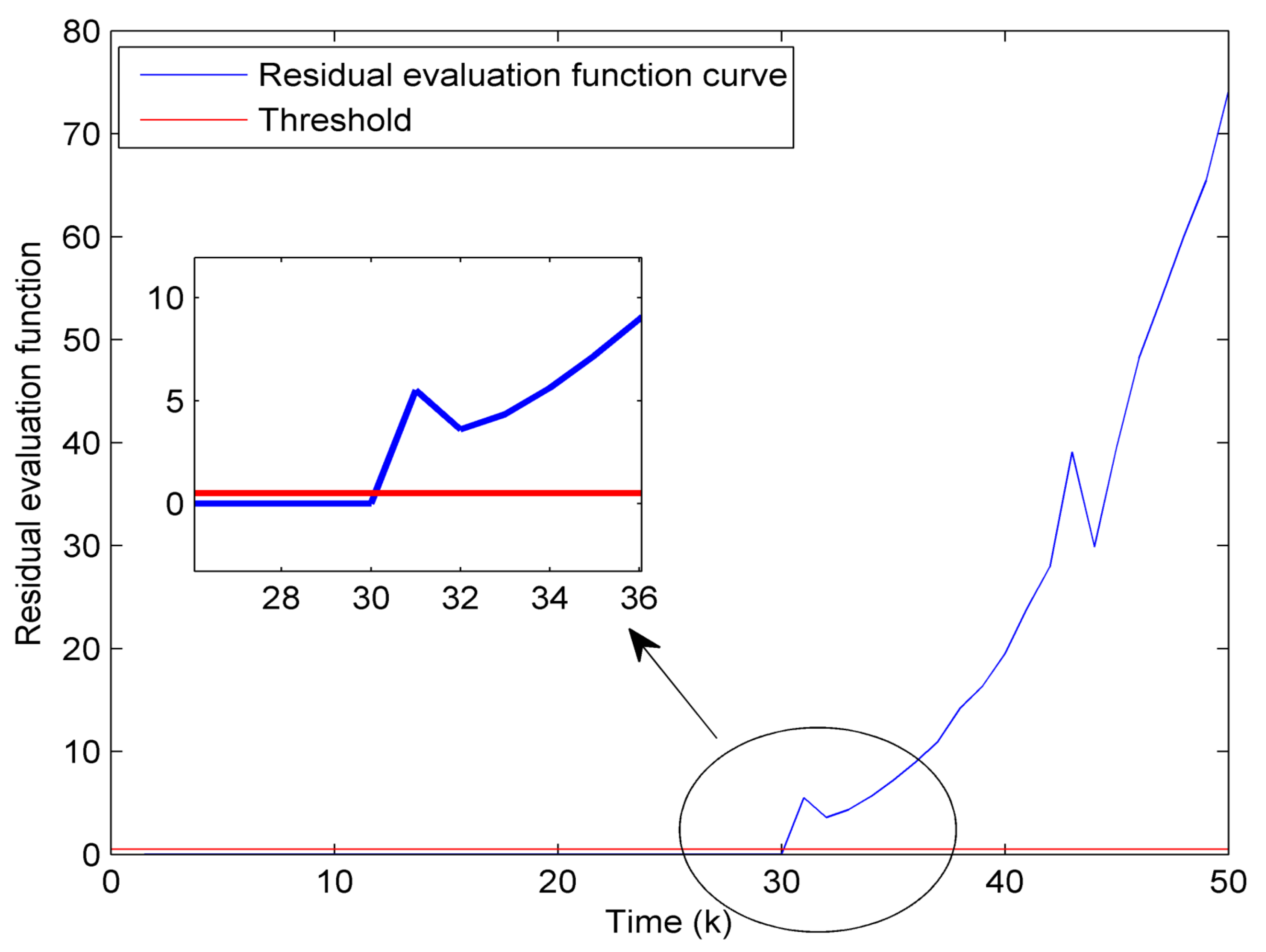
Step 1: Design an event-triggered fault-detection filter of the form in Equation (13) based on the design procedure of Algorithm 1.
Step 2: Calculate fault-detection residual generator r k in Equation (14).
Step 3: Determine the residual evaluation function r T and the threshold J t h .
Step 4: If r T is above the threshold J t h , then a fault is detected and the corresponding fault alarm can be turned on. Otherwise, the system is healthy.
End
Remark 7.
In [22], an event-triggered reduced-order fault-detection filter is derived where a copy of remote fault-detection filter is employed at the sensor side to avoid the delay issue of fault-alarming. Comparatively, the fault-alarming strategy described in Algorithm 2 of this paper is less additional computing burden than that in [22] because the local fault-detection filter is not required in this paper. Furthermore, the proposed strategy also could be an excellent fault-alarm, which is verified via an experimental example in the next section.

4. Application to Event-Triggered Fault Detection of a One-Dimensional Target Tracking

4.1. Target Tracking Description and Modeling

In this subsection, a one-dimensional target tracking [43] is simulated to demonstrate the effectiveness of the proposed event-triggered fault-detection approach. The dynamic model of the considered one-dimensional target tracking is described by
x k + 1 = 1 τ 0 1 x k + τ 2 / 2 τ d k y k = x k + d k
where τ and d k are the sampling period and the unknown acceleration, respectively. Target state x k = p k T , p ˙ k T T and y k is the sensor information at time k. The variables p k and p ˙ k denote the target position and velocity, respectively. In this example, the sampling period τ = 0 . 1 . Sensor nonlinearity is assumed that s η = 1 . 7 S 1 + S 2 η + 0 . 3 S 1 S 2 sin η where S 1 = 0 . 3 and S 2 = 0 . 15 . The probability of sensor nonlinearity is chosen as 6 % . Furthermore, the physical constraints imposed on the attack signal are characterized by M ̲ = 0 . 6 and M ¯ = 1 . 6 . The disturbances is selected as d k = ε k = 0 . 4 e 0 . 8 k . Other Parameters are chosen as A 2 = 0 . 15 0 0 . 1 0 . 2 , D 1 = D 2 = 0 . 3 and F 1 = F 2 = 1 . With the aforementioned parameters, the fault-detection filter gains and event conditions can be derived by solving linear matrix inequalities in Theorem 1 and 2: γ 1 = 0 . 35 , γ 2 = 0 . 02 , λ 1 = 9 . 761 , λ 2 = 0 . 02928 , V = d i a g [ 1 , 1 ] and L 10 2 × 7 . 51 0 . 139 0 . 2043 6 . 91 .

4.2. Assessment of Effectiveness of the Designed Fault-Detection Filter

In this subsection, we test the efficiency of the proposed event-triggered fault-detection filter by the following experiments.
Experiment 1: Robustness on Event-Triggered Filter
To compare the estimation performance, the state estimation trajectories without fault f k are shown in Figure 1a,b which reveal comparison between our filter using event-triggered data-transmission (ED) and the proposed filter using periodical data-transmission (PD). The event-triggered transmission behaviors are also illustrated in Figure 1c. As shown in Figure 1, two lines are almost coincident as time increases. Obviously, the estimation accuracy is not affected by the event-triggered data transmission scheme.
Further, to verify the estimation performance clearly, the effect on event-triggered filter is examined subject to the different probabilities of sensor nonlinearity. Table 1 shows the root mean-square estimation error (RMEE) of system state 1 corresponding to increased probabilities. One can see that the estimation performance degrades slightly as β increases.
Experiment 2: Security on Event-Triggered Filter.
As illustrated in Figure 1, predefined deception attacks cannot affect the filter estimation accuracy. However, different deception attacks may lead to the different estimation performance. In this experiment, the estimation performance is evaluated subject to different false information ε k sent by attackers. Constant false information, time-varying false information and unbounded false information are respectively created as ε k = 0 . 1 , ε k = 0 . 1 sin 0 . 15 k and ε k = 0 . 1 e 0 . 2 k .
The root mean-square estimation error curves are shown in Figure 2 for the CPS subject to different deception attacks. One can see that the estimation error convergence is guaranteed under the constant false information and time-varying false information. However, as shown in Figure 2, it is a pity that the proposed filter is infeasible for the unbounded deception attacks.
Experiment 3: Sensitivity, robustness and real-time capability of fault detection
Here, two fault scenarios are considered as follow:
  • an incipient fault:
    f k = 0 k 30 0 . 02 e 0 . 08 k otherwise
  • a sudden-changing fault:
    f k = 0 k 30 k otherwise
For d ˜ k = 0 , the residual evaluation function responses for an incipient fault (Equation (32)) and a sudden-changing fault (Equation (33)) are demonstrated in Figure 3 and Figure 4, respectively. The same responses with the above given d ˜ k are demonstrated in Figure 5 and Figure 6. It can be noted that the proposed residual can not only detect the fault in time, but also identifies the system fault from the influence of disturbance d k and false information ε k .
Experiment 4: Energy Conservation Effect on a Wireless Node.
In the final experiment, an experimental node is applied to test its lifetime to verify whether the proposed event-triggered scheme is energy-saving. As shown in Figure 7, the node includes the following components: (i) a STM32F103 micro-controller (computation module) with ARM cortex-M3 CPU determines when to transmit data packets via our event-triggered scheme; (ii) an ESP8266 wireless transceiver (wireless communication module) transmits data packets from sensor to remote fault-detection filter; (iii) a 75 mAh lithium-polymer battery system (power management module) ensures a constant voltage output received from the Lithium-ion battery; and (iv) a digital voltmeter is regarded as a battery lifetime monitoring system. Please refer to the user manuals [44,45] for more information about this node. The relationship between time and voltage for periodical and event-triggered scheme is illustrated in Figure 8. It is not difficult to find that the final battery lifetime for periodical and event-triggered data-transmission are 30 min and 34 min, respectively. In other words, the battery life is extended by 11.7%, and thus the wireless node can be used for a longer time to become more energy-efficient.
Remark 8.
It is observed from Figure 8 that the voltage of the battery is 3.9 V completely charged. The voltage of the battery using the periodical data-transmission has dropped to 3 V after 28 min. This indicates that the presented wireless node cannot work normally since its working voltage must exceed 3 V [44,45].

5. Conclusions and Future Work

The problem of event-triggered fault detection for stochastic CPSs was investigated in this work. The addressed system was subject to randomly occurring sensor nonlinearities, additive disturbances and deception attacks. Using the stochastic stability analysis, the closed-loop estimation error dynamics were mean-square stable under the proposed event condition. On the other hand, two performance criteria were utilized for the design of fault-detection residual to achieve the robustness of unwanted factors d ˜ k and the sensitivity of faults f k , respectively. Finally, an application example of one-dimensional target tracking was illustrated to obtain the benefits of the proposed event-triggered fault-detection approach by comparative simulations. The wireless node platform clearly verified conservative consumption of the battery energy. Even though the event-triggered transmission scheme is always used to improve the battery lifetime of sensor networks of CPSs, the threshold monitoring significantly affects the power consumption in practice [46]. Hence, the self-triggered scheme may be an interesting direction for prevent such monitoring [47,48] in CPSs.

Author Contributions

Y.L. conceived, designed, performed, and analyzed the experiments and wrote the paper under the guidance of L.P. and X.L.

Funding

This research was funded by National Key R&D Program of China (No. 2018YFD0400900); Education Ministry and China Mobile Science Research Foundation (No. MCM20170204), respectively.

Acknowledgments

The authors wish to thank the anonymous referees and the Editor for providing many invaluable comments and suggestions that led to significant improvement of the paper. Without their help, the paper would not be in its present shape.

Conflicts of Interest

The authors declare no conflict of interest.

Appendix A. Proof of Theorem 1

Proof. 
The Lyapunov function is constructed as follows
V k = e k T P 1 e k + x k T P 2 x k
where P j j = 1 a n d 2 are symmetric positive definite matrices. It follows from Equations (1) and (15) that
Δ V k = E V k + 1 e k , , e 0 , x k , , x 0 V k = A 1 β L C e k + A d e k d L M ^ D 2 d k L M ̲ ε k L ϕ y a , k β 1 L M ^ s C ¯ x k + A 2 x k + D 1 d k w k T P 1 A 1 β L C e k + A d e k d L M ^ D 2 d k L M ̲ ε k L ϕ y a , k L M ^ D 2 d k L M ̲ ε k L ϕ y a , k β 1 L M ^ s C ¯ x k + A 2 x k + D 1 d k w k + A 1 x k + A d x k d + A 2 x k + D 1 d k w k T P 2 A 1 x k + A d x k d + A 2 x k + D 1 d k w k + E β k β 2 L C x k + L M ^ s C ¯ x k T P 1 L C x k + L M ^ s C ¯ x k + e k T P 3 P 1 e k + x k T P 4 P 2 x k e k d T P 3 e k d x k d T P 4 x k d
where β 1 = 1 β , M ^ = I M ̲ and C = I M ̲ C ¯ . Because β 2 = Δ E β k β 2 = β β 2 and the conditions in Equations (3) and (8) are satisfied, the above equation can be formulated that
Δ V k e k T A 1 β L C T P 1 A 1 β L C + P 3 P 1 e k + e k d T A d T P 1 A d P 3 e k d + ϕ T y a , k L T P 1 L ϕ y a , k + β 1 2 s T C ¯ x k M ^ T L T P 1 L M ^ s C ¯ x k + x k T A 2 T P 1 + P 2 A 2 x k + 2 e k T A 1 β L C T P 1 A d e k d 2 e k T A 1 β L C T P 1 L ϕ y a , k 2 β 1 e k T A 1 β L C T P 1 L M ^ s C ¯ x k 2 e k d T A d T P 1 L ϕ y a , k 2 β 1 e k d T A d T P 1 L M ^ s C ¯ x k + 2 β 1 ϕ T y a , k L T P 1 L M ^ s C ¯ x k + x k T A 1 T P 2 A 1 + P 4 P 2 x k + x k d T A d T P 2 A d P 4 x k d + 2 x k T A 1 T P 2 A d x k d + β 2 x k T C T L T P 1 L C x k s T C ¯ x k s C ¯ x k + 2 β 2 x k T C T L T P 1 L M ^ s C ¯ x k β ϕ T y a , k M ˜ C ¯ x k x k T C ¯ T S 1 T S 2 C ¯ x k + 2 x k T S 2 C ¯ + S 1 C ¯ 2 T s C ¯ x k ϕ T y a , k ϕ y a , k β 1 ϕ T y a , k M ˜ s C ¯ x k + β 2 s T C ¯ x k M ^ T L T P 1 L M ^ s C ¯ x k = η k T Λ η k
where η k = e k T e k d T ϕ T y a , k s T C ¯ x k x k T x k d T T . Without considering the disturbance d ˜ k and using the inequality in Equation (18), one can obtain that
Δ V k = E V k + 1 e k , , e 0 , x k , , x 0 V k = η k T Λ η k λ min Λ η k T η k α 1 η k T η k
where 0 < α 1 < min λ min Λ , α 2 and α 2 = max λ max P 1 , λ max P 2 . From Equation (A4), the following inequality can be deduced that
E Δ V k α 1 η k T η k < α 1 α 2 V k
which satisfies conditions of Lemma 1. Therefore, the dynamic error system in Equation (15) is mean-square stable for d ˜ k according to Definition 1. Now, we consider the influence of unknown disturbance d ˜ k and introduce the following criterion
J 1 = k = 0 E r k T r k γ 1 2 k = 0 E d ˜ k T d ˜ k
where d ˜ k = d k T ε k T T . For any nonzero d ˜ k 2 0 , and zero initial condition, one has
J 1 = k = 0 E r k T r k γ 1 2 E d ˜ k T d ˜ k + Δ V k V k
which further results in
E r k T r k γ 1 2 E d ˜ k T d ˜ k + Δ V k = β 2 e k T C T V T V C e k + β 1 2 s T C ¯ x k M ^ T V T V M ^ s C ¯ x k + d k T D 2 T M ^ T V T V M ^ D 2 d k + ε k T M ̲ T V T V M ̲ ε k + ϕ T y a , k V T V ϕ y a , k + β 2 s T C ¯ x k M ^ T V T V M ^ s C ¯ x k + β 2 x k T C T V T V C x k + 2 β β 1 e k T C T V T V M ^ s C ¯ x k + 2 β e k T C T V T V M ^ D 2 d k + 2 β e k T C T V T V M ̲ ε k + 2 β e k T C T V T V ϕ y a , k + 2 β 1 s T C ¯ x k M ^ T V T V M ^ D 2 d k + 2 β 1 s T C ¯ x k M ^ T V T V M ̲ ε k + 2 β 1 s T C ¯ x k M ^ T V T V ϕ y a , k + 2 d k T D 2 T M ^ T V T V ε k + 2 d k T D 2 T M ^ T V T V ϕ y a , k + 2 ε k T M ̲ T V T V ϕ y a , k 2 β 2 s T C ¯ x k M ^ T V T V C x k γ 1 2 d ˜ k T d ˜ k + Δ V k = η d , k T Λ η d , k
where η d , k = e k T e k d T ε k T ϕ T y a , k s T C ¯ x k x k T x k d T d k T T . By using the Schur lemma and the notation R = P 1 L , we deduce that the inequality in Equation (A8) is equivalent to Equation (15), i.e., η d , k T Λ η d , k < 0 . Consequently, the condition in Equation (15) guarantees J 1 < 0 for any k, which implies that E r k 2 < γ 1 2 E d ˜ k 2 . □

Appendix B. Proof of Theorem 2

Proof. 
It is obvious that Equation (24) implies Equation (18), hence it follows from Theorem 1 that the estimator in Equation (13) in the presence of the disturbance-free case is exponentially mean-square stable. Next, for any nonzero f k and zero initial condition, a performance index function is introduced as
J 2 = k = 0 E r k T r k γ 2 2 E f k T f k Δ V k + V k
where Δ V k = E V k + 1 e k , , e 0 , x k , , x 0 V k , and define the increment of V k along the trajectories of Equation (15) in the disturbance-free case. It turns out
Δ V k E r k T r k + γ 2 2 E f k T f k = β 2 e k T C T V T V C e k + β 1 2 s T C ¯ x k M ^ T V T V M ^ s C ¯ x k + f k T F 2 T M ^ T V T V M ^ F 2 f k + ϕ T y a , k V T V ϕ y a , k + β 2 s T C ¯ x k M ^ T V T V M ^ s C ¯ x k + β 2 x k T C T V T V C x k + 2 β β 1 e k T C T V T V M ^ s C ¯ x k + 2 β e k T C T V T V M ^ F 2 f k + 2 β e k T C T V T V ϕ y a , k + 2 β 1 s T C ¯ x k M ^ T V T V M ^ F 2 f k + 2 β 1 s T C ¯ x k M ^ T V T V ϕ y a , k + γ 2 2 f k T f k + Δ V k + 2 f k T F 2 T M ^ T V T V ϕ y a , k 2 β 2 s T C ¯ x k M ^ T V T V C x k = η f , k T Λ η f , k
where
η f , k = e k T e k d T ϕ T y a , k s T C ¯ x k x k T x k d T f k T T
With the help of the inequality in Equation (24), we have
Δ V k E r k T r k + γ 2 2 E f k T f k < 0
Now, summing up Equation (A12) from 0 to with respect to k yields
k = 0 E r k 2 > γ 2 2 k = 0 E f k 2 + E V E V 0
which is straightforward to see that
k = 0 E r k 2 > γ 2 2 k = 0 E f k 2
 □

References

  1. Seshia, S.A.; Hu, S.; Li, W.; Zhu, Q. Design Automation of Cyber-Physical Systems: Challenges, Advances, and Opportunities. IEEE Trans. Comput. Aided Des. Integr. Circuits Syst. 2017, 36, 1421–1434. [Google Scholar] [CrossRef]
  2. Naghshtabrizi, P.; Joa, B.; Xu, Y. A Survey of Recent Results in Networked Control Systems. Proc. IEEE 2007, 95, 138–162. [Google Scholar] [CrossRef] [Green Version]
  3. Pandey, A.; Tripathi, R.C. A Survey on Wireless Sensor Networks Security. Int. J. Comput. Appl. 2010, 3, 43–49. [Google Scholar] [CrossRef] [Green Version]
  4. Sridhar, B.S.; Hahn, A.; Govindarasu, M. Cyber-Physical System Security for the Electric Power Grid. Proc. IEEE 2012, 100, 210–224. [Google Scholar] [CrossRef]
  5. Khaitan, S.K.; Member, S.; Mccalley, J.D. Design Techniques and Applications of Cyberphysical Systems: A Survey. IEEE Syst. J. 2015, 9, 350–365. [Google Scholar] [CrossRef]
  6. Sang, C.S.; Tanik, U.J.; Carbone, J.N.; Eroglu, A. Applied Cyber-Physical Systems; Springer: New York, NY, USA, 2014. [Google Scholar]
  7. Zhang, K.; Jiang, B.; Shi, P. Observer-based integrated robust fault estimation and accommodation design for discrete-time systems. Int. J. Control 2010, 83, 1167–1181. [Google Scholar] [CrossRef]
  8. Jia, Q.; Chen, W.; Zhang, Y.; Li, H. Fault Reconstruction and Fault-tolerant Control via Learning Observers in Takagi-Sugeno Fuzzy Descriptor Systems with Time Delays. IEEE Trans. Ind. Electron. 2015, 62, 3885–3895. [Google Scholar] [CrossRef]
  9. Li, Y.; Peng, L. Event-Triggered Fault Estimation for Stochastic Systems over Multi-Hop Relay Networks with Randomly Occurring Sensor Nonlinearities and Packet Dropouts. Sensors 2018, 18, 731. [Google Scholar] [CrossRef] [PubMed]
  10. Alavi, S.M.M.; Saif, M.; Member, S. Fault Detection in Nonlinear Stable Systems over Lossy Networks. IEEE Trans. Control Syst. Technol. 2013, 21, 2129–2142. [Google Scholar] [CrossRef]
  11. Chen, W.; Chen, W.T.; Saif, M.; Li, M.F.; Wu, H. Simultaneous Fault Isolation and Estimation of Lithium-Ion Batteries via Synthesized Design of Luenberger and Learning Observers. IEEE Trans. Control Syst. Technol. 2014, 22, 290–298. [Google Scholar] [CrossRef]
  12. Li, Y.; Peng, L. Event-triggered sensor data transmission policy for receding horizon recursive state estimation. J. Algor. Comput. Technol. 2017, 11, 178–185. [Google Scholar] [CrossRef]
  13. Miskowicz, M. Event-Based Control and Signal Processing; CRC Press: Boca Raton, FL, USA, 2016. [Google Scholar]
  14. Xie, C.; Li, Y.; Xie, Y.; Wang, H.; Peng, L. On Kalman Filter for Stochastic System with Correlated Noises Based on Event-Triggered Sampling. In Proceedings of the China Control Conference, Chengdu, China, 27–29 July 2016; pp. 8330–8334. [Google Scholar]
  15. Shi, D.; Shi, L.; Chen, T. Event-Based State Estimation. A Stochastic Perspective; Springer: Berlin, Germany, 2016. [Google Scholar]
  16. Niu, Y.; Ho, D.W.C.; Li, C.W. Filtering For Discrete Fuzzy Stochastic Systems with Sensor Nonlinearities. IEEE Trans. Fuzzy Syst. 2010, 18, 971–978. [Google Scholar] [CrossRef]
  17. Miskowicz, M. Send-on-Delta Concept: An Event-Based Data Reporting Strategy. Sensors 2006, 6, 49–63. [Google Scholar] [CrossRef]
  18. Suh, Y.S. Send-on-delta sensor data transmission with a linear predictor. Sensors 2007, 7, 537–547. [Google Scholar] [CrossRef]
  19. Sijs, J.; Lazar, M. On event-based state estimation. In Proceedings of the International Workshop on Hybrid Systems: Computation and Control, Rome, Italy, 28–30 March 2001; pp. 336–350. [Google Scholar]
  20. Miskowicz, M. Event-based sampling strategies in networked control systems. In Proceedings of the IEEE Workshop on Factory Communication Systems, Toulouse, France, 5–7 May 2014; pp. 1–10. [Google Scholar]
  21. Trimpe, S.; Campi, M.C. On the choice of the event trigger in event-based estimation. In Proceedings of the 1st International Conference on Event-Based Control, Communication and Signal Processing, Krakow, Poland, 17–19 June 2014; pp. 1–8. [Google Scholar]
  22. Li, Y.; Li, P.; Chen, W. An energy-efficient data transmission scheme for remote state estimation and applications to a water-tank system. ISA Trans. 2017, 70, 494–501. [Google Scholar] [CrossRef] [PubMed]
  23. Gao, Y.; Li, Y.; Peng, L. Design of Event-Triggered Fault-Tolerant Control for Stochastic Systems with Time-Delays. Sensors 2018, 18, 1929. [Google Scholar] [CrossRef] [PubMed]
  24. Socas, R.; Dormido, R.; Dormido, S. New control paradigms for resources saving: An approach for mobile robots navigation. Sensors 2018, 18, 281. [Google Scholar] [CrossRef] [PubMed]
  25. Hu, Y.; Lu, Q.; Hu, Y. Event-Based Communication and Finite-Time Consensus Control of Mobile Sensor Networks for Environmental Monitoring. Sensors 2018, 18, 2547. [Google Scholar] [CrossRef] [PubMed]
  26. Diaz-Cacho, M.; Delgado, E.; Barreiro, A.; Falcón, P. Basic send-on-delta sampling for signal tracking-error reduction. Sensors 2017, 17, 312. [Google Scholar] [CrossRef] [PubMed]
  27. Putra, I.; Brusey, J.; Gaura, E.; Vesilo, R. An event-triggered machine learning approach for accelerometer-based fall detection. Sensors 2018, 18, 20. [Google Scholar] [CrossRef] [PubMed]
  28. Xu, Z.; Liu, G.; Yan, H.; Cheng, B.; Lin, F. Trail-based search for efficient event report to mobile actors in wireless sensor and actor networks. Sensors 2017, 17, 2468. [Google Scholar] [CrossRef] [PubMed]
  29. Santos, C.; Martínez-Rey, M.; Espinosa, F.; Gardel, A.; Santiso, E. Event-based sensing and control for remote robot guidance: An experimental case. Sensors 2017, 17, 2034. [Google Scholar] [CrossRef] [PubMed]
  30. Acho, L. Event-Driven Observer-Based Smart-Sensors for Output Feedback Control of Linear Systems. Sensors 2017, 17, 2028. [Google Scholar] [CrossRef] [PubMed]
  31. Wang, D.; Wang, Z.; Shen, B.; Alsaadi, F.E. Security-guaranteed filtering for discrete-time stochastic delayed systems with randomly occurring sensor saturations and deception attacks. Int. J. Robust Nonlinear Control 2017, 27, 1194–1208. [Google Scholar] [CrossRef]
  32. Li, Y.; Wu, Q.; Li, P. Simultaneous Event-Triggered Fault Detection and Estimation for Stochastic Systems Subject to Deception Attacks. Sensors 2018, 18, 321. [Google Scholar] [CrossRef] [PubMed]
  33. Li, Y.; Shi, L.; Cheng, P.; Chen, J.; Quevedo, D.E. Jamming Attacks on Remote State Estimation in Cyber-Physical Systems : A Game-Theoretic Approach. IEEE Trans. Autom. Control 2015, 60, 2831–2836. [Google Scholar] [CrossRef]
  34. Zemouche, A.; Boutayeb, M. Observer Design for Lipschitz Nonlinear Systems: The Discrete-Time Case. IEEE Trans. Circuits Syst. II Express Briefs 2006, 53, 777–781. [Google Scholar] [CrossRef]
  35. Cao, Y.; Member, S.; Lin, Z.; Chen, B.M.; Member, S. An Output Feedback H Controller Design for Linear Systems Subject to Sensor Nonlinearities. IEEE Trans. Circuits Syst. I Fundam. Theory Appl. 2003, 50, 914–921. [Google Scholar] [CrossRef]
  36. Pan, Y.; Li, H.; Zhou, Q. Fault detection for interval type-2 fuzzy systems with. Neurocomputing 2014, 145, 488–494. [Google Scholar] [CrossRef]
  37. Wen, J.; Peng, L.; Kiong, S. Stochastic finite-time boundedness on switching dynamics Markovian jump linear systems with saturated and stochastic nonlinearities. Inf. Sci. 2016, 334–335, 65–82. [Google Scholar] [CrossRef]
  38. Wang, Z.; Ho, D.W.C.; Dong, H.; Gao, H. Robust Finite-Horizon H Control for a Class of Stochastic Nonlinear Time-Varying Systems Subject to Sensor and Actuator Saturations. IEEE Trans. Autom. Control 2010, 55, 1716–1722. [Google Scholar] [CrossRef]
  39. Li, Q.; Shen, B.; Liu, Y.; Huang, T. Event-triggered H state estimation for discrete-time neural networks with mixed time delays and sensor saturations. Neural Comput. Appl. 2016, 28, 3815–3825. [Google Scholar] [CrossRef]
  40. Ma, L.; Wang, Z.; Han, Q.; Lam, H. Variance-Constrained Distributed Filtering for Time-Varying Systems With Multiplicative Noises and Deception Attacks over Sensor Networks. IEEE Sens. J. 2017, 17, 2279–2288. [Google Scholar] [CrossRef]
  41. Ding, D.; Wang, Z.; Ho, D.W.C.; Wei, G. Distributed recursive filtering for stochastic systems under uniform quantizations and deception attacks through sensor networks. Automatica 2017, 78, 231–240. [Google Scholar] [CrossRef]
  42. He, S.; Liu, F. Fuzzy model-based fault detection for Markov jump systems. Int. J. Robust Nonlinear Control 2009, 19, 1248–1266. [Google Scholar] [CrossRef]
  43. Li, W.; Jia, Y.; Du, J. Event-triggered state estimator for stochastic systems with unknown inputs. IET Signal Process. 2016, 11, 1–6. [Google Scholar] [CrossRef]
  44. STM32F103RC Instructions, STMicroelectronics. Available online: https://www.st.com/resource/en/datasheet/stm32f103rc.pdf (accessed on 30 November 2017).
  45. ESP8266 Instructions, Espressif Systems. Available online: https://www.espressif.com/en/support/download/overview (accessed on 30 November 2017).
  46. Park, P.; Coleri Ergen, S.; Fischione, C.; Lu, C.; Johansson, K.H. Wireless Network Design for Control Systems: A Survey. IEEE Commun. Surv. Tutor. 2018, 20, 978–1013. [Google Scholar] [CrossRef] [Green Version]
  47. Araujo, J.; Mazo, M.; Anta, A.; Tabuada, P.; Johansson, K.H. System architectures, protocols and algorithms for aperiodic wireless control systems. IEEE Trans. Ind. Inform. 2014, 10, 175–184. [Google Scholar] [CrossRef]
  48. Wang, X.; Lemmon, M.D. Self-triggered feedback control systems with finite-gain L2 stability. IEEE Trans. Autom. Control 2009, 54, 452–467. [Google Scholar] [CrossRef]
Figure 1. State estimation trajectories without fault f k and the corresponding event-triggered transmission behaviors.
Electronics 07 00168 g001
Figure 2. The root mean-square estimation error curves under different deception attacks.
Electronics 07 00168 g002
Figure 3. The residual evaluation function responses of the system with zero d ˜ k for an incipient fault (Equation (32)).
Electronics 07 00168 g003
Figure 4. The residual evaluation function responses of the system with zero d ˜ k for a sudden-changing fault (Equation (33)).
Electronics 07 00168 g004
Figure 5. The residual evaluation function responses of the system with d ˜ k for an incipient fault (Equation (32)).
Electronics 07 00168 g005
Figure 6. The residual evaluation function responses of the system with d ˜ k for a sudden-changing fault (Equation (33)).
Electronics 07 00168 g006
Figure 7. A photograph of the wireless node.
Electronics 07 00168 g007
Figure 8. The relationship between time and voltage for periodical and event-triggered scheme.
Electronics 07 00168 g008
Table 1. Root mean-square estimation error (RMEE) of system state 1 with the increased probabilities.
Sensor Nonlinearity Probabilities β = 0 . 1 β = 0 . 15 β = 0 . 2 β = 0 . 25 β = 0 . 3 β = 0 . 35
RMEE0.0920.1970.21760.23630.25010.2901

