The Impact of Antenna Height on 3D Channel: A Ray Launching Based Analysis

 ,
,
Abstract
1. Introduction
2. Methods and Numerical Results
2.1. Intelligent Ray Launching Algorithm (IRLA)
2.2. Numerical Results
3. Results
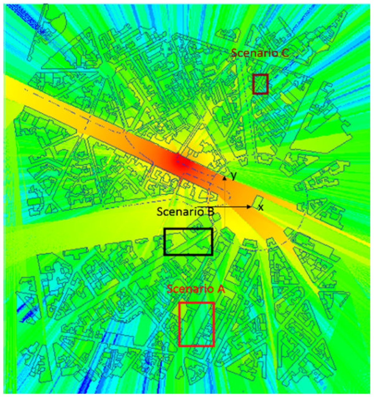
3.1. Scenario A: Straight Street in the Center of Paris
3.2. Scenario B: Forked Road in the Center of Paris
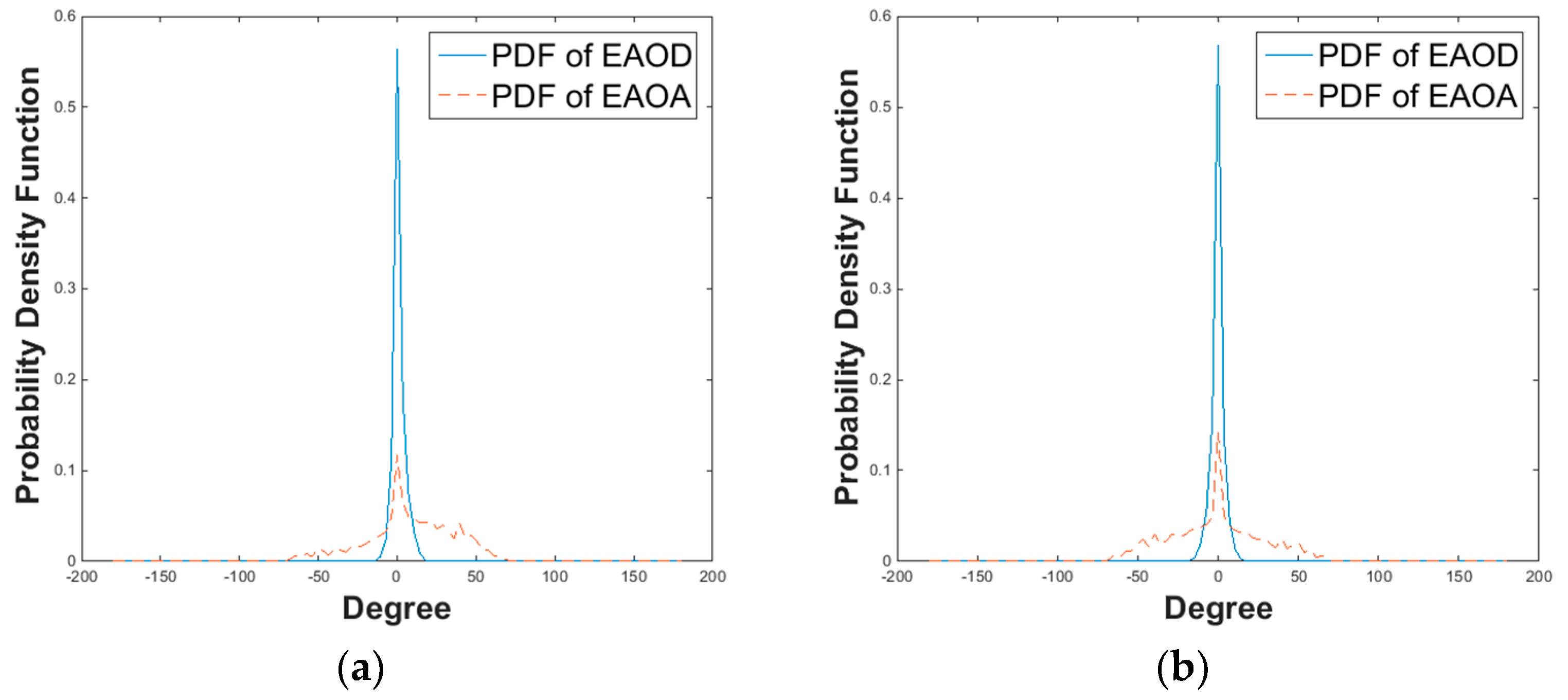
- For the PDF of EAoD: the logarithm exponent value λ′1EAoD is nearly unchangeable when the antenna height is lower than half of the building’s height, but has a dramatic increase when the antenna height grows. However, the logarithm exponent value λ′2EAoD enhances when the antenna height is lower than half of the building’s height and then remains stable.
- For the PDF of EAoA: the logarithm exponent value λ′1EAoA decreases rapidly when the antenna height is lower than half of the building’s height and then varies slightly. However, the logarithm exponent value λ′2EAoA is almost stable when the antenna height is lower than half of the building’s height, but has a significant drop when the antenna height increases.
3.3. Scenario C: Crossroad in the Center of Paris
- For the PDF of EAoD: the logarithm exponent value λ′1EAoD reduces rapidly when the antenna height is lower than half of the building’s height, and gains the minimum value at 14 m, and then the value remains the same. In contrast, the logarithm exponent value λ′2EAoD is nearly unchangeable when the antenna height is lower than half of the building’s height, but has a dramatic decrease when the antenna height grows.
- For the PDF of EAoA: the exponent value decreases λ′1EAoA as the antenna height rises. In contrast, the exponent value λ′2EAoA is nearly unchanged when the antenna height is lower than half of the building’s height, but has a significantly drop when the antenna height increases.
3.4. Discussion
4. Conclusions
Acknowledgments
Author Contributions
Conflicts of Interest
References
- David, L.P.; Guvenc, I.; de la Roche, G.; Kountouris, M.; Quek, T.Q.S.; Zhang, J. Enhanced intercell interference coordination challenges in heterogeneous networks. IEEE Wirel. Commun. 2011, 18, 22–30. [Google Scholar]
- Almesaeed, R.N.; Ameen, A.S.; Mellios, E.; Doufexi, A.; Nix, A. 3D channel models: Principles, Characteristics, and System Implications. IEEE Commun. Mag. 2017, 55, 152–159. [Google Scholar] [CrossRef]
- Ertel, R.B.; Reed, J.H. Angle and time of arrival statistics for circular and elliptical scattering models. IEEE J. Sel. Areas Commun. 1999, 11, 1829–1840. [Google Scholar] [CrossRef]
- Khan, N.M.; Simsim, M.T.; Rapajic, P.B. A generalized model for the spatial characteristics of the cellular mobile channel. IEEE Trans. Veh. Technol. 2008, 1, 22–37. [Google Scholar] [CrossRef]
- Haenggi, M.; Andrews, J.G.; Baccelli, F.; Dousse, O.; Franceschetti, M. Stochastic geometry and random graphs for the analysis and design of wireless networks. IEEE J. Sel. Areas Commun. 2009, 7, 1029–1046. [Google Scholar] [CrossRef]
- Molisch, A.F. Modeling of directional wireless propagation channels. URSI Radio Sci. Bull. 2002, 302, 16–26. [Google Scholar]
- Jakes, W.C.; Cox, D.C. Microwave Mobile Communications; Wiley-IEEE Press: New York, NY, USA, 1994. [Google Scholar]
- Mahmoud, S.S.; Hussain, Z.M.; Peter, O.S. A space-time model for mobile radio channel with hyperbolically distributed scatterers. IEEE Antennas Wirel. Propag. Lett. 2002, 1, 211–214. [Google Scholar] [CrossRef]
- Alsehaili, M.; Noghanian, S.; Buchan, D.A.; Sebak, A.R. Angle-of-Arrival statistics of a three-dimensional geometrical scattering channel model for indoor and outdoor propagation environments. IEEE Antennas Wirel. Propag. Lett. 2010, 9, 946–949. [Google Scholar] [CrossRef]
- Kammoun, A.; Khanfir, H.; Altman, Z.; Debbah, M.; Kamoun, M. Preliminary results on 3DD channel modelling: From theory to standardization. IEEE J. Sel. Areas Commun. 2014, 32, 1219–1229. [Google Scholar] [CrossRef]
- Aulin, T. A modified model for the fading Signal at a mobile radio channel. IEEE Trans. Veh. Technol. 1979, 28, 182–203. [Google Scholar] [CrossRef]
- Taga, T. Analysis for mean effective gain of mobile antennas in land mobile radio environments. IEEE Trans. Veh. Technol. 1990, 39, 117–131. [Google Scholar] [CrossRef]
- Petrus, P.; Reed, J.H.; Rappaport, T.S. Geometrical-based statistical macrocell channel model for mobile environments. IEEE Trans. Commun. 2002, 3, 495–502. [Google Scholar] [CrossRef]
- Shafi, M. The impact of elevation angle on MIMO capacity. In Proceedings of the IEEE International Conference on Communications, Istanbul, Turkey, 11–15 June 2006; pp. 4155–4160. [Google Scholar]
- Nawaz, S.J. A generalized 3-D scattering model for a macrocell environment with a directional antenna at the BS. IEEE Trans. Veh. Technol. 2010, 7, 3193–3204. [Google Scholar] [CrossRef]
- Tzarouchis, D.C.; Ylä-Oijala, P.; Sihvola, A. Resonant scattering characteristics of homogeneous dielectric sphere. IEEE Trans. Antennas Propag. 2017, 6, 3184–3191. [Google Scholar] [CrossRef]
- Qu, S.; Yeap, T. A Three-dimensional scattering model for fading channels in land mobile environment. IEEE Trans. Veh. Technol. 1999, 3, 765–781. [Google Scholar]
- Kalliola, K.; Sulonenet, K.; Laitinen, H.; Kivekas, O.; Krogerus, J.; Vainikainen, P. Angular power distribution and mean effective gain of mobile antenna in different propagation environments. IEEE Trans. Veh. Technol. 2002, 5, 823–838. [Google Scholar] [CrossRef]
- Mondal, B.; Thomas, T.A.; Visotsky, E.; Vook, F.W.; Ghosh, A.; Nam, Y.-H.; Li, Y.; Zhang, J.; Zhang, M. 3D channel model in 3GPP. IEEE Commun. Mag. 2015, 3, 16–23. [Google Scholar] [CrossRef]
- Ballot, M. Radio-wave propagation prediction model tuning of land cover effects. IEEE Trans. Veh. Technol. 2014, 8, 3490–3498. [Google Scholar] [CrossRef]
- Kurner, T. Radio Wave Propagation Part One “Theoretical Aspects”; COST2100 Training School: Wroclaw, Poland, 2008. [Google Scholar]
- Lostanlen, Y. Radio Wave Propagation Part Two “Practical Aspects”; COST2100 Training School: Wroclaw, Poland, 2008. [Google Scholar]
- Klepal, M. Novel Approach to Indoor Electromagnetic Wave Propagation Modelling. Ph.D. Thesis, Czech Technical University, Prague, Czech, 2003. [Google Scholar]
- Janaswamy, R. Angle and time of arrival statistics for the Gaussian scatter density model. IEEE Trans. Wirel. Commun. 2002, 3, 488–497. [Google Scholar] [CrossRef]
- Hoppe, R.; Wolfle, G.; Landstorfer, F. Accelerated ray optical propagation modelling for the planning of wireless communication networks. In Proceedings of the 1999 IEEE Radio and Wireless Conference, Denver, CO, USA, 1–4 August 1999. [Google Scholar]
- Lai, Z.; Bessis, N.; de la Roche, G.; Song, H.; Zhang, J.; Clapworthy, G. An intelligent ray launching for urban propagation prediction. In Proceedings of the 3rd European Conference on Antennas and Propagation, Berlin, Germany, 23–27 March 2009; pp. 2867–2871. [Google Scholar]
- Lai, Z.; Bessis, N.; Kuonen, P.; de la Roche, G.; Zhang, J.; Clapworthy, G. A performance evaluation of a grid-enabled object-oriented parallel outdoor ray launching for wireless network coverage prediction. In Proceedings of the Fifth International Conference on Wireless and Mobile Communications, Cannes, France, 23–29 August 2009; pp. 38–43. [Google Scholar]
- Lai, Z.; Bessis, N.; de la Roche, G.; Kuonen, P.; Zhang, J.; Clapworthy, G. A new approach to solve angular dispersion of discrete ray launching for urban scenarios. In Proceedings of the Loughborough Antennas & Propagation Conference, Loughborough, UK, 16–17 November 2009; pp. 133–136. [Google Scholar]
- Lai, Z.; Bessis, N.; de la Roche, G.; Kuonen, P.; Zhang, J.; Clapworthy, G. The characterisation of human-body influence on indoor 3.5 GHz path loss measurement. In Proceedings of the 2010 IEEE Wireless Communications and Networking Conference Workshops (WCNCW), Sydney, Australia, 18 April 2010. [Google Scholar]
- Umansky, D.; de la Roche, G.; Lai, Z.; Villemaud, G.; Gorce, J.-M.; Zhang, J. A new deterministic hybrid model for indoor-to-outdoor radio coverage prediction. In Proceedings of the 5th European Conference on Antennas and Propagation (EUCAP), Rome, Italy, 11–15 April 2011; pp. 3771–3774. [Google Scholar]
- de la Roche, G.; Flipo, P.; Lai, Z.; Villemaud, G.; Zhang, J.; Gorce, J.-M. Combination of geometric and finite difference models for radio wave propagation in outdoor to indoor scenarios. In Proceedings of the Fourth European Conference on Antennas and Propagation (EuCAP), Barcelona, Spain, 12–16 April 2010. [Google Scholar]
- de la Roche, G.; Gorce, J.-M.; Zhang, J. Optimized implementation of the 3D MR-FDPF method for indoor radio propagation prediction. In Proceedings of the 3rd European Conference on Antennas and Propagation, Berlin, Germany, 23–27 March 2009. [Google Scholar]
- de la Roche, G.; Flipo, P.; Lai, Z.; Villemaud, G.; Zhang, J.; Gorce, J.-M. Implementation and validation of a new combined model for outdoor to indoor radio coverage predictions. Wirel. Commun. Netw. 2010, 2010, 215352. [Google Scholar] [CrossRef]
- Weng, J.; Tu, X.; Lai, Z.; Salous, S.; Zhang, J. LaiIndoor Massive MIMO Channel Modelling Using Ray-Launching Simulation. Int. J. Antenna Propag. 2014, 2014, 279380. [Google Scholar] [CrossRef] [PubMed]
- Ranplan. The Role and Benefits of RF and Performance Modelling Tools in the HetNet Era. White Paper. 2015. Available online: https://ranplanwireless.com/wp-content/uploads/The-Role-and-Benefits-of-RF-and-Performance-Modelling-tools-in-HetNet-Era.pdf (accessed on 7 November 2017).
- Donikian, S. Vuems: A virtual urban environment modelling system. In Proceedings of the Computer Graphics IntHasselt and Diepenbeek, Belgium, Hasselt and Diepenbeek, Belgium, 23–27 June 1997; pp. 84–92. [Google Scholar]


| Size of Area | Average Buildings Height | BS Power | Carrier Frequency | BS Antenna Type | Max Reflection Number | Max Diffraction Number |
|---|---|---|---|---|---|---|
| 500 m × 300 m | 21 m | 0 dBm | 2.4 GHz | Omnidirectional 4 × 1 | 3 | 7 |
| Average Buildings Height | Length of Wider Street | Width of Wider Street | Length of Lower Street | Width of Lower Street | |
|---|---|---|---|---|---|
| Straight street | 20 m | 80 m | 20 m | 0 m | 0 m |
| Forked road | 25 m | 80 m | 20 m | 40 m | 12 m |
| Crossroad | 22 m | 40 m | 20 m | 40 m | 12 m |
| 4 m | 6 m | 8 m | 10 m | 12 m | 14 m | 16 m | 18 m | |
|---|---|---|---|---|---|---|---|---|
| EAoD down | 40.19 | 32.86 | 32.31 | 33.16 | 33.16 | 33.25 | 34.58 | 36.2 |
| EAoD up | −32.49 | −35.89 | −34.23 | −33.67 | −32.63 | −32.99 | −32.93 | −32.94 |
| EAoA down | 17.4 | 20.92 | 19.11 | 18 | 17.69 | 17.94 | 17.95 | 18.03 |
| EAoA up | −18.06 | −16.2 | −15.77 | −16 | −17.06 | −16.64 | −16.45 | −18.68 |
| 4 m | 6 m | 8 m | 10 m | 12 m | 14 m | 16 m | 18 m | |
|---|---|---|---|---|---|---|---|---|
| EAoD down | 199 | 149.8 | 118.3 | 110.5 | 88.88 | 79.08 | 85.5 | 79.05 |
| EAoD up | −79.57 | −87.87 | −76.54 | −85.21 | −103 | −113.1 | −131.2 | −172.7 |
| EAoA down | 19.52 | 17.72 | 14.08 | 12.08 | 12.87 | 10.91 | 9.77 | 11.1 |
| EAoA up | −9.556 | −12.86 | −10.7 | −11.25 | −13.12 | −13.46 | −15.32 | −19.56 |
© 2018 by the authors. Licensee MDPI, Basel, Switzerland. This article is an open access article distributed under the terms and conditions of the Creative Commons Attribution (CC BY) license (http://creativecommons.org/licenses/by/4.0/).
Share and Cite
Hong, Q.; Zhang, J.; Zheng, H.; Li, H.; Hu, H.; Zhang, B.; Lai, Z.; Zhang, J. The Impact of Antenna Height on 3D Channel: A Ray Launching Based Analysis. Electronics 2018, 7, 2. https://doi.org/10.3390/electronics7010002
Hong Q, Zhang J, Zheng H, Li H, Hu H, Zhang B, Lai Z, Zhang J. The Impact of Antenna Height on 3D Channel: A Ray Launching Based Analysis. Electronics. 2018; 7(1):2. https://doi.org/10.3390/electronics7010002
Chicago/Turabian StyleHong, Qi, Jiliang Zhang, Hui Zheng, Hao Li, Haonan Hu, Baoling Zhang, Zhihua Lai, and Jie Zhang. 2018. "The Impact of Antenna Height on 3D Channel: A Ray Launching Based Analysis" Electronics 7, no. 1: 2. https://doi.org/10.3390/electronics7010002
APA StyleHong, Q., Zhang, J., Zheng, H., Li, H., Hu, H., Zhang, B., Lai, Z., & Zhang, J. (2018). The Impact of Antenna Height on 3D Channel: A Ray Launching Based Analysis. Electronics, 7(1), 2. https://doi.org/10.3390/electronics7010002