Antenna Design by Means of the Fruit Fly Optimization Algorithm

Abstract

In this work a heuristic optimization algorithm known as the Fruit fly Optimization Algorithm is applied to antenna design problems. The original formulation of the algorithm is presented and it is adapted to array factor and horn antenna optimization problems. Specifically, it is applied to the array factor synthesis of uniformly-fed, non-equispaced arrays and to the profile optimization of multimode horn antennas. Several numerical examples are presented and the obtained results are compared with those provided by a deterministic optimization based on a simplex method and another well-known heuristic approach, the Genetic Algorithm.

1. Introduction

The design of microwave and millimetre-wave devices is tightly related to optimization processes. In the first stages of the design process a circuital approximation of the problem may be used in some cases (e.g., filters, couplers, etc.), and the parameters of this circuit can be optimized to obtain an initial design of the device. Nevertheless, these approximations do not take complex electromagnetic effects into account. Therefore, in complex designs an optimization of a proper full-wave model of the device is necessary to fine tune the main parameters of the device and obtain the final design.

Many optimization processes are based on deterministic routines that traditionally make use of the derivatives of a certain cost function. Nevertheless, modern computational power allows the use of heuristic or evolutionary techniques such as the Genetic Algorithm (GA) [1,2,3,4,5], Ant Colony Optimization (ACO) [6,7,8], Particle Swarm Optimization (PSO) [9,10,11,12], or Gravitational Search Algorithm (GSA) [13,14] among others. These algorithms are especially suited for problems where the derivative of the cost function is unknown or not easily computed. Additionally, they are also less prone to get stuck at a local minima of the cost function than the techniques based on derivatives.

In this work, one of these algorithms, known as the Fruit fly Optimization Algorithm (FOA) [15], is presented and adapted for its application to the design of antenna devices. This algorithm was created to study financial distress models [15] and it has also been successfully applied to other problems [16,17]. Nevertheless, the application of this algorithm to antenna design optimization has been very limited; few examples exist in the literature [18,19] and all of them are dedicated to the synthesis of array factor analytical functions.

To illustrate the performance of the implemented algorithm different numerical examples are presented. Specifically, the FOA will be first applied to the problem of synthesizing an array factor (as an initial validation example) and then to the more complex case of the optimization of horn antenna profiles, which are of primary interest in the front-end of modern communication systems [3,4]. To the best of the authors’ knowledge the FOA has not been applied to complex radiation problems like these, which require full wave simulations.

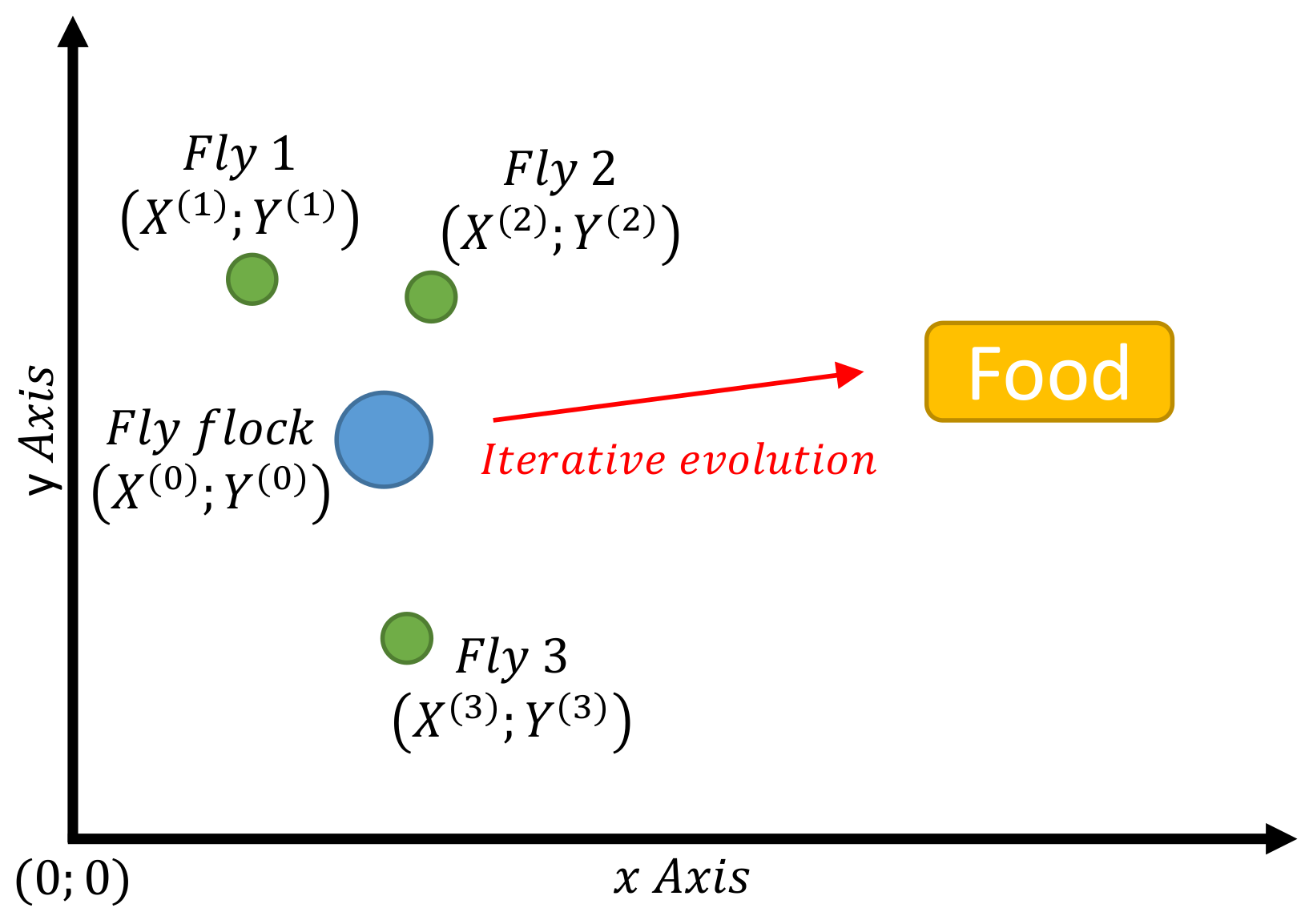
2. Description of the Algorithm

The FOA is based on the food searching behaviour of a swarm of fruit flies. These insects are capable of finding food kilometres away from their location by using two mechanisms: osphresis and vision. The osphresis organs of each fly in a swarm can smell all types of scents and make each fly move according to its osphresis sensing. Then, after each fly gets close to the estimated food location following its own smell concentration judgement, the whole swarm moves by using vision towards the fly whose location provides the actual highest smell concentration of food [15].

The computational implementation of the algorithm repeats this process for a defined number of iterations. The flies move in a two-dimensional space with coordinates X and Y, and the parameters to be optimized are related to the smell concentration judgement of each fly.

Consequently, in each iteration of the FOA, the following steps must be carried out:

• The swarm is positioned at the location $(X^{\left(0\right)};Y^{\left(0\right)})$, with a given smell concentration $Smel{l}^{\left(0\right)}$. For each fly i in the swarm:
  • The fly moves around a random distance, searching for food by using the osphresis:

    $$X^{\left(i\right)}=X^{\left(0\right)}+R^X,Y^{\left(i\right)}=Y^{\left(0\right)}+R^Y,$$

    (1)

    where $R^X$ and $R^Y$ are random values.
  • The smell concentration judgement value is defined as the reciprocal of the distance to the origin of coordinates:

    $$S^{\left(i\right)}=\frac{1}{\sqrt{{\left(X^{\left(i\right)}\right)}^2+{\left(Y^{\left(i\right)}\right)}^2}}$$

    (2)
  • Compute the smell concentration of the fly’s current location by using the smell concentration function (equivalent to a fitness function):

    $$Smel{l}^{\left(i\right)}=Function(S^{\left(i\right)})$$

    (3)
• Look for the specific fly I with the best smell concentration. If this value is better than the value in the initial location of the swarm $(X^{\left(0\right)};Y^{\left(0\right)})$ then move the swarm towards the position of the fly I by using the vision sense:

  $$X^{\left(0\right)}=X^{\left(I\right)},Y^{\left(0\right)}=Y^{\left(I\right)}$$

  (4)

The described behaviour of the algorithm is represented in Figure 1.

In order to guarantee that the FOA converges, and that this convergence is reached in a reasonable amount of time, two important factors must be considered: the initial positions of the fly swarms and the generation of the random values $R^X$ and $R^Y$.

The swarm positions could be initialized randomly, but a significantly faster convergence can be achieved by using some prior knowledge of the problem, as it is typical with heuristic algorithms, and manually initializing them to values in the range of the solution values, making a rough approximation.

The random values $R^X$ and $R^Y$ are generated using a uniform distribution. The interval of this distribution must be chosen carefully since if it is very big the search will be erratic and the algorithm will have trouble converging to a maximum. On the other hand, if it is too small the search will be very slow and, in addition, the risk of getting stuck in a local maximum of the smell function (equivalent to a minimum of a cost function) will be larger.

As it happens with most of these heuristic techniques, this FOA description may recall to another algorithm of this family like, in this case, the PSO. Nevertheless, it is worth mentioning that despite their similarities there are usually subtle but relevant differences between these algorithms. As an example, the particles of PSO present inertia, whereas the flies of FOA do not.

3. Numerical Examples

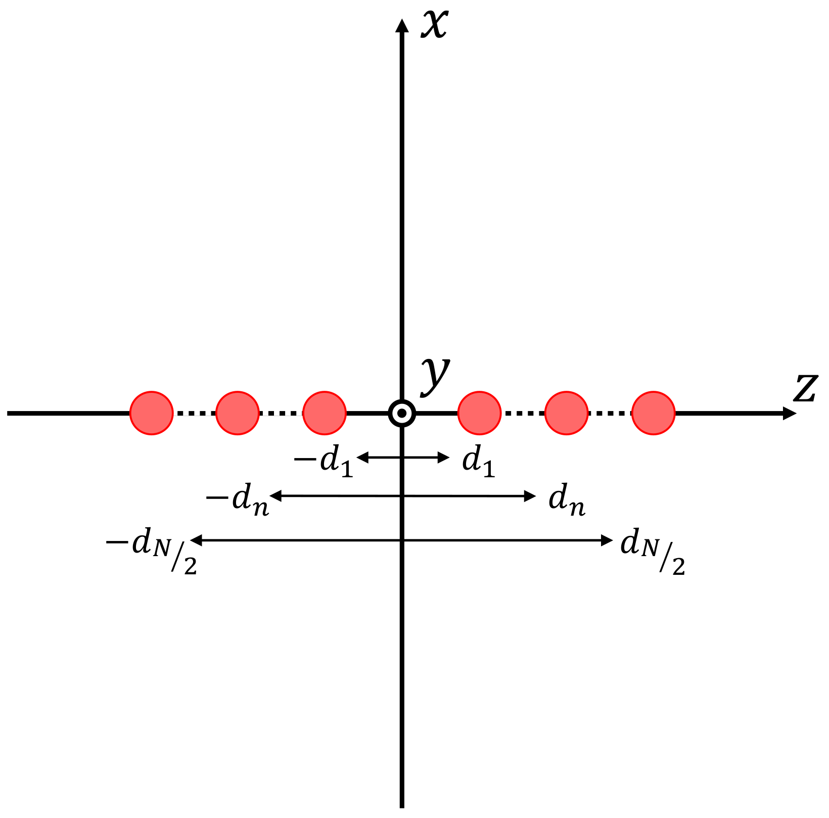
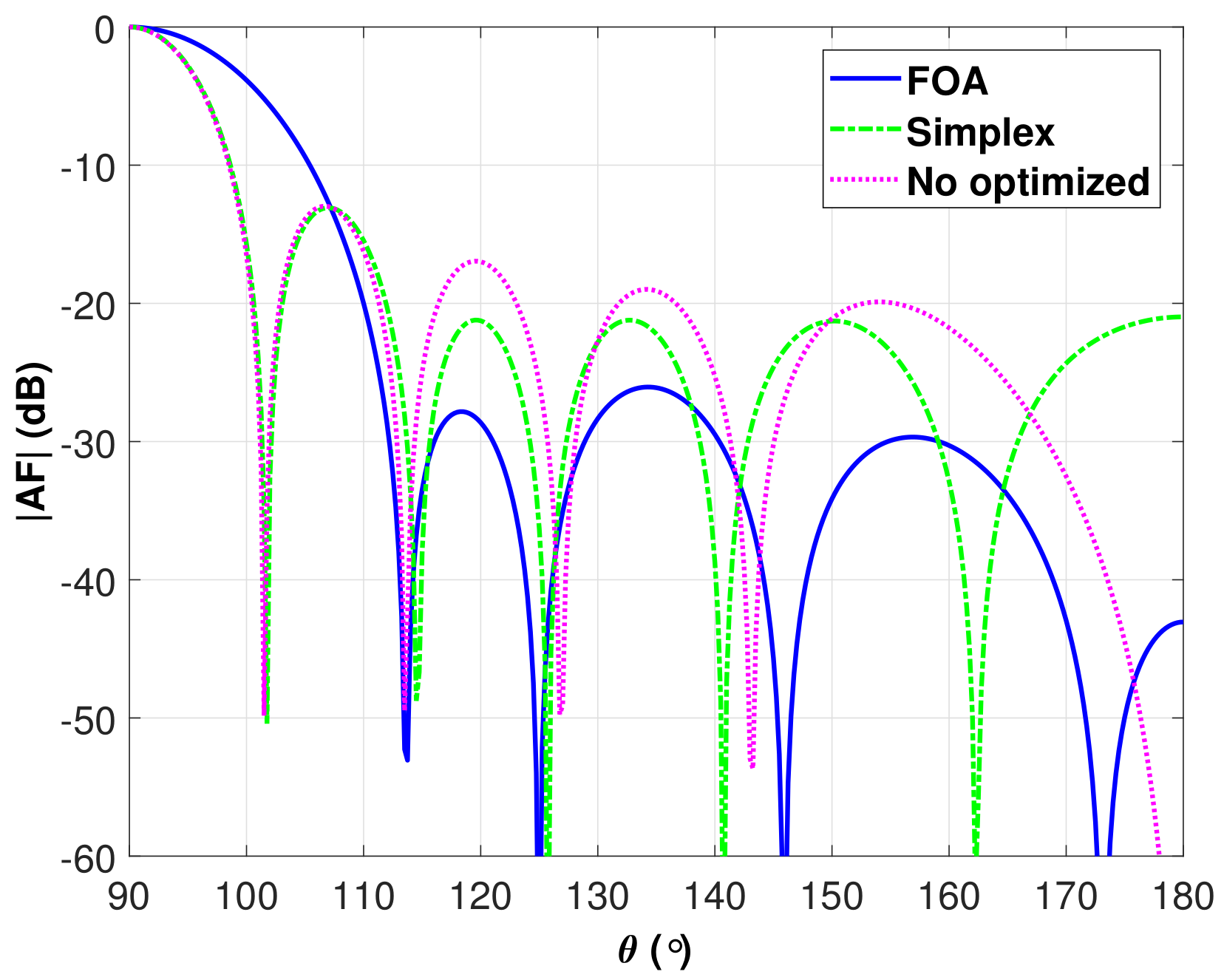
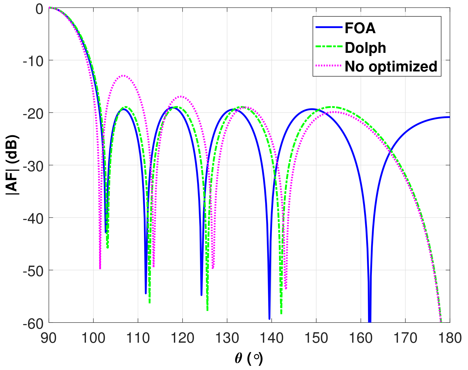
3.1. Application to Array Factor Synthesis

As an initial proof of concept the implemented FOA has been applied to the problem of optimizing an array factor. This example has been chosen since the evaluation of the required smell function is not computationally expensive and therefore it allows for a faster testing of the implemented algorithm. In the next section a problem with a more sophisticated smell function will be presented.

The antenna arrays studied in the following examples will be linear (placed along the $\widehat{\mathbf{z}}$ axis) and use an even number of antennas distributed symmetrically with respect to the $XY$ plane. A schematic representation of this kind of arrays is depicted in Figure 2.

The process of synthesizing a desired array factor consists in choosing the appropriate excitation coefficient and position for each element. Uniformly-fed (all the excitation coefficients have the same amplitude) arrays are an interesting option in antenna systems since they require a simpler feeding network. The arrays studied in the following examples will be of this kind, which implies that the array factor will be optimized by only modifying the spacing between the unitary elements.

Therefore, the particular array factor for the numerical examples will be

$$AF\left(\theta \right)=\sum _{n=1}^{N/2}cos(k_0·d_n·cos\left(\theta \right)),$$

(5)

where $k_0=2\pi /{\lambda }_0$ and $d_n$ is the position of the nth element (${\lambda }_0=c_0/f_0$ being the free-space wavelength at the operating frequency $f_0$). The spherical coordinate system used in this work is represented in Figure 3.

Since this is a multivariate problem (there are $N/2$ positions to optimize), several swarms are required to apply the FOA. Each one of the swarms will be associated to the position of one element [20].

The smell concentration function has to be defined in terms of the desired array factor (side lobe level (SLL), directivity, null directions, etc.). Specifically, the presented optimization examples pursue the lowest possible SLL and therefore the employed smell function will be

$$Smell=\underset{m}{max}\left[20·{log}_{10}\left(\frac{\left|AF\right({\theta }_0\left)\right|}{\left|AF\right({\theta }_m\left)\right|}\right)\right],$$

(6)

where ${\theta }_m$ represents the directions outside the main beam.

The first example will aim at, starting from an equispaced array, reducing the SLL as much as possible without increasing the beamwidth more than 4${}^{\circ }$ through the modification of the positions of the uniformly-fed elements. The optimization results will be compared with those provided by a Dolph synthesis [21], since, as it is known, the Dolph synthesis produces an equispaced array with the narrowest beamwidth for a certain SLL level through the proper determination of every excitation amplitudes (which in our optimization will be required to remain all equal).

The number of isotropic elements used for the synthesis is $N=10$ and the initial spacing between the elements is $d={\lambda }_0/2$. It is known that the beamwidth between the first pair of null directions of such an array is ${22}^{\circ }$ and its SLL is $-13$ dB when all elements are uniformly excited [21]. Therefore, the main beam region is defined in the $Smell$ function as ${79}^{\circ }\le \theta \le {101}^{\circ }$ (note that, since the array is placed along the $\widehat{\mathbf{z}}$ axis, the broadside direction is ${\theta }_0={90}^{\circ }$).

The employed settings (heuristically determined) of the FOA have been the following:

• Flies per swarm: 20.
• Total smell function evaluations: 5000.

After the optimization the achieved array factor has an SLL of −18.93 dB (the optimized positions of the elements can be found at

Table 1. Element positions of the first array factor synthesis example.

Parameter	Initial / Dolph	FOA
$d_1$	$0.250{\lambda }_0$	$0.2029{\lambda }_0$
$d_2$	$0.750{\lambda }_0$	$0.5260{\lambda }_0$
$d_3$	$1.250{\lambda }_0$	$1.0812{\lambda }_0$
$d_4$	$1.750{\lambda }_0$	$1.6361{\lambda }_0$
$d_5$	$2.250{\lambda }_0$	$2.2917{\lambda }_0$

). The array factor is represented in Figure 4, compared with that of a Dolph synthesis for the same SLL. It can be seen that the optimized array factor achieves the same beamwidth and therefore the FOA results can be considered satisfactory since, as it was mentioned, the Dolph synthesis produces the narrowest possible beam for a certain SLL.

It is important to emphasize again that the main difference between the two arrays lies on the fact that whereas the Dolph synthesis produces an equispaced but not uniformly excited array, the optimized array is uniformly excited (same excitation for all elements) and not equispaced. The latter type has the advantage of requiring a simpler feeding network.

The second example studies how much the FOA can decrease the SLL of the array factor when a significant increase of the beamwidth is permitted. For this example, the main beam region will be defined as ${68}^{\circ }\le \theta \le {112}^{\circ }$ (double beamwidth than in the equispaced, uniformly-excited case) and the initial spacing will be the same as the previous example ($d=0.5{\lambda }_0$). In this case the results will be compared against those of a deterministic optimization using a Simplex method.

The FOA settings (number of flies and number of smell function evaluations) are the same than in the previous example, 20 flies per swarm and 5000 evaluations of the smell function. In the case of the simplex optimization the cost function has also been evaluated 5000 times.

The obtained element positions can be found at

Table 2. Element positions of the second array factor synthesis example.

Parameter	Initial	FOA	Simplex
$d_1$	$0.250{\lambda }_0$	$0.0789{\lambda }_0$	$0.2710{\lambda }_0$
$d_2$	$0.750{\lambda }_0$	$0.3149{\lambda }_0$	$0.7540{\lambda }_0$
$d_3$	$1.250{\lambda }_0$	$0.8228{\lambda }_0$	$1.2320{\lambda }_0$
$d_4$	$1.750{\lambda }_0$	$0.7631{\lambda }_0$	$1.6840{\lambda }_0$
$d_5$	$2.250{\lambda }_0$	$1.4619{\lambda }_0$	$2.2580{\lambda }_0$

and the corresponding array factors are represented in Figure 5. It can be seen that whereas the FOA optimization has significantly improved the SLL of the initial setup (equispaced array) providing an SLL of $-26$ dB, the Simplex optimization has not significantly improved the array factor since it seems to have gotten stuck in a local minimum. This example shows one of the main advantages of FOA: it, as other heuristic techniques, can avoid local minima better than most of the deterministic methods.

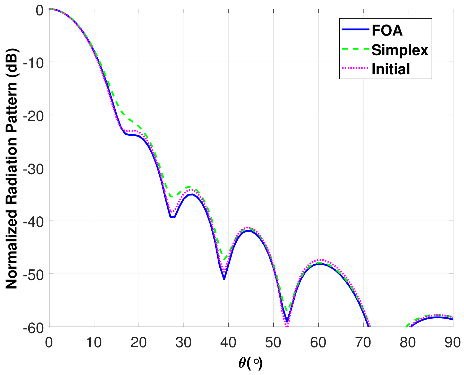
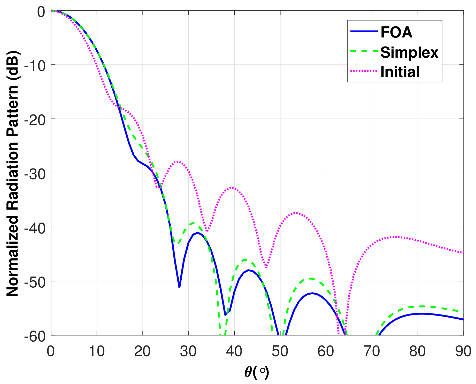
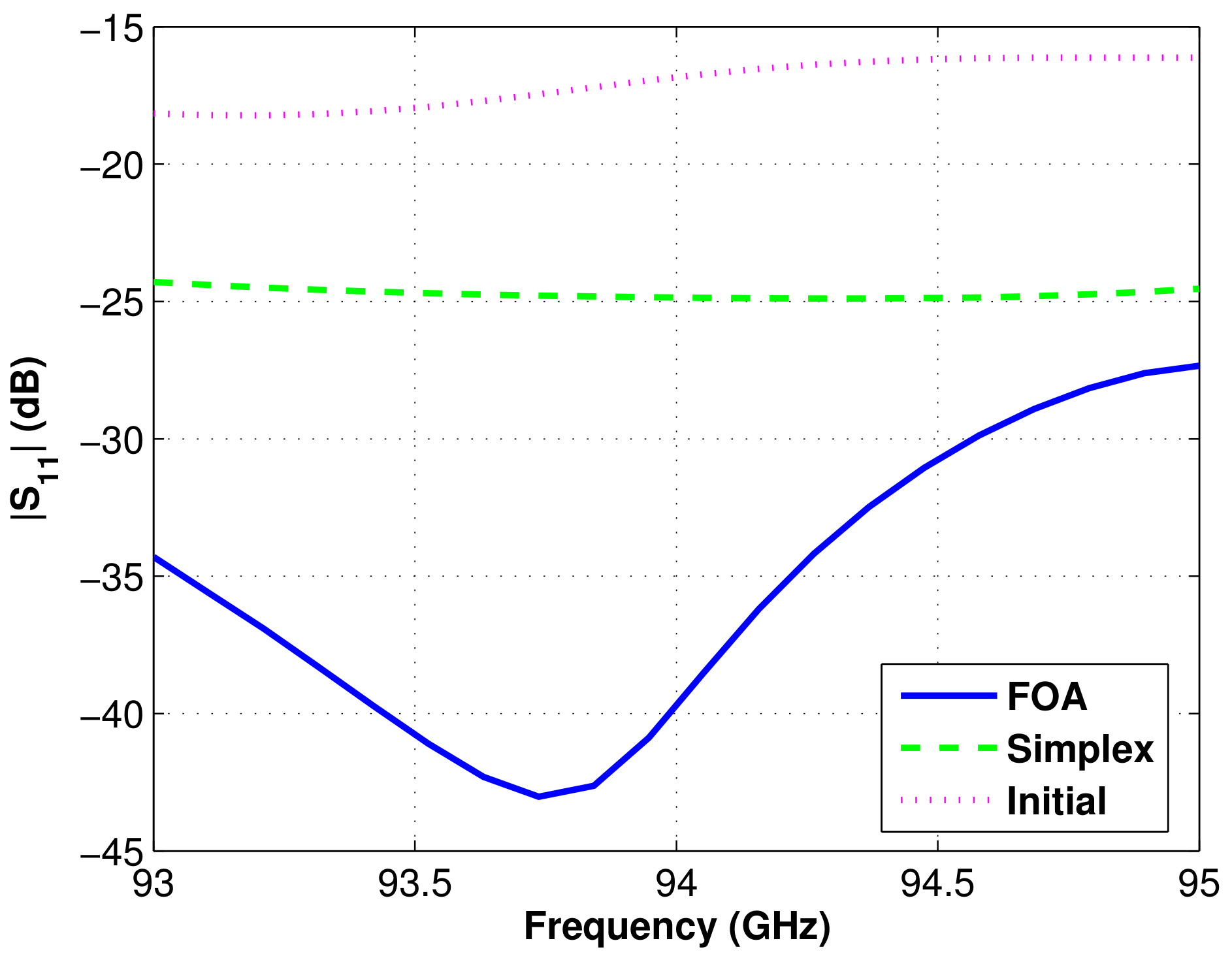
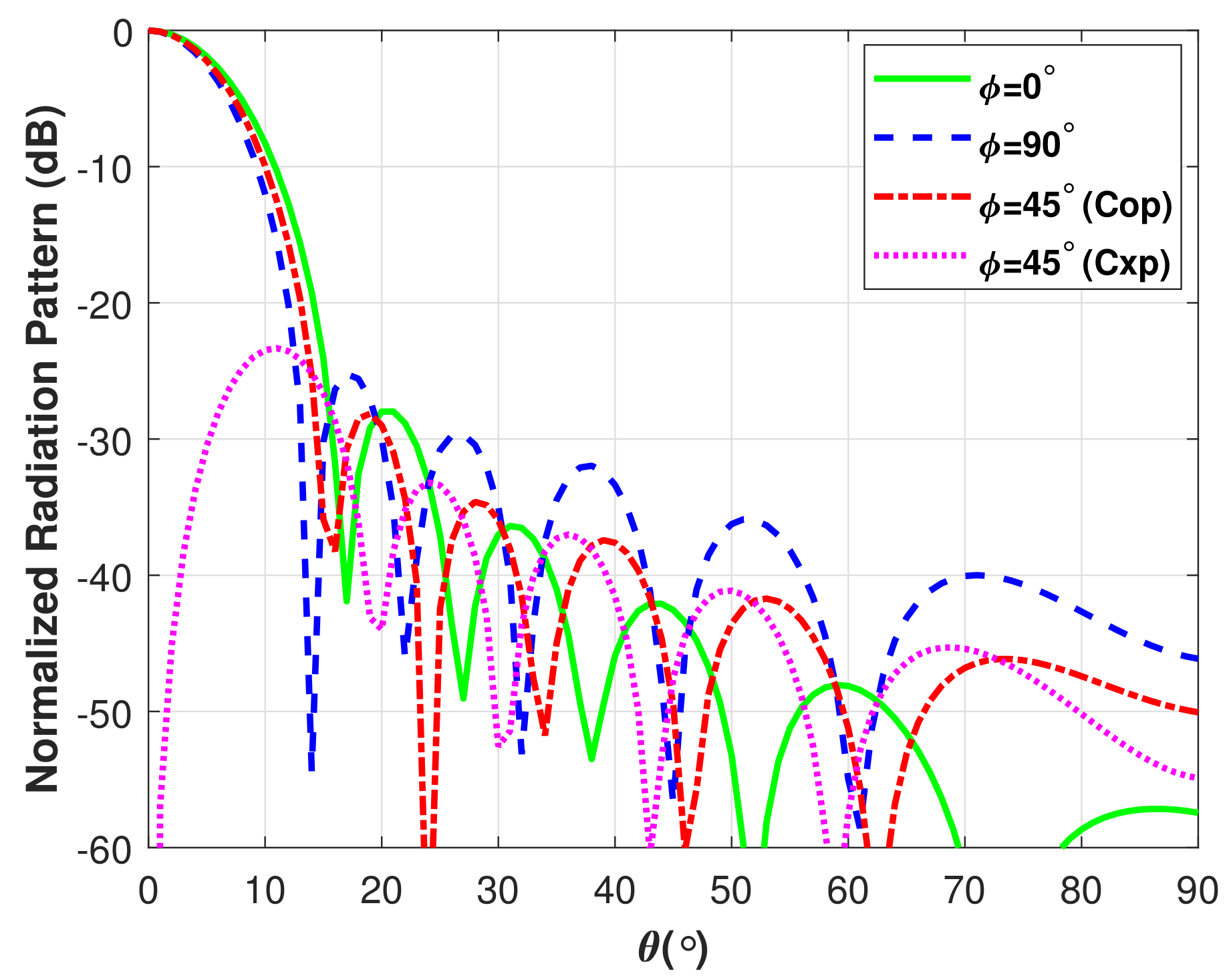
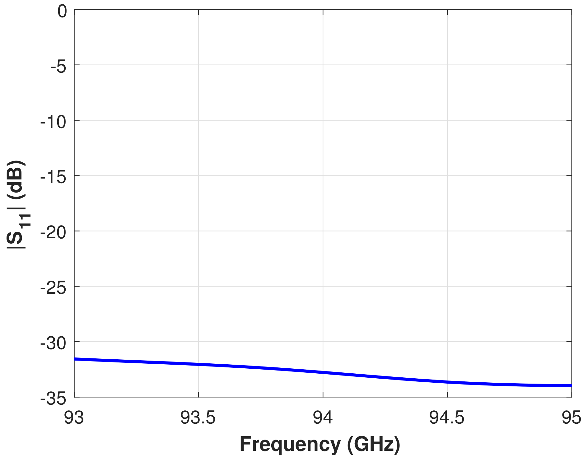
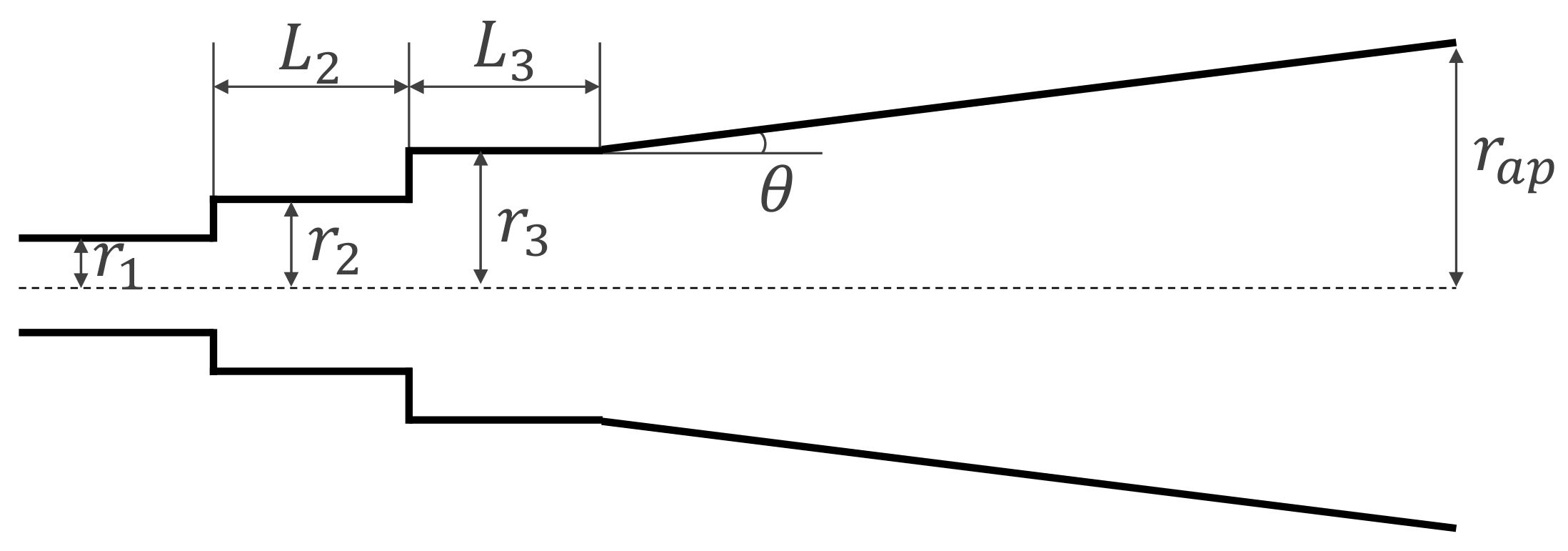
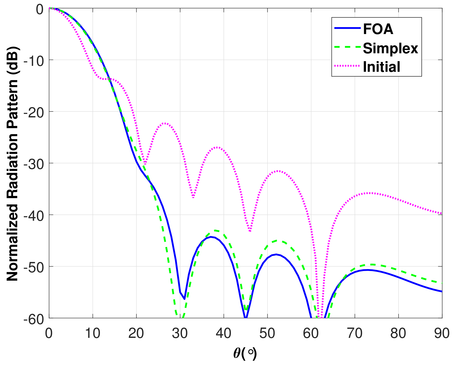
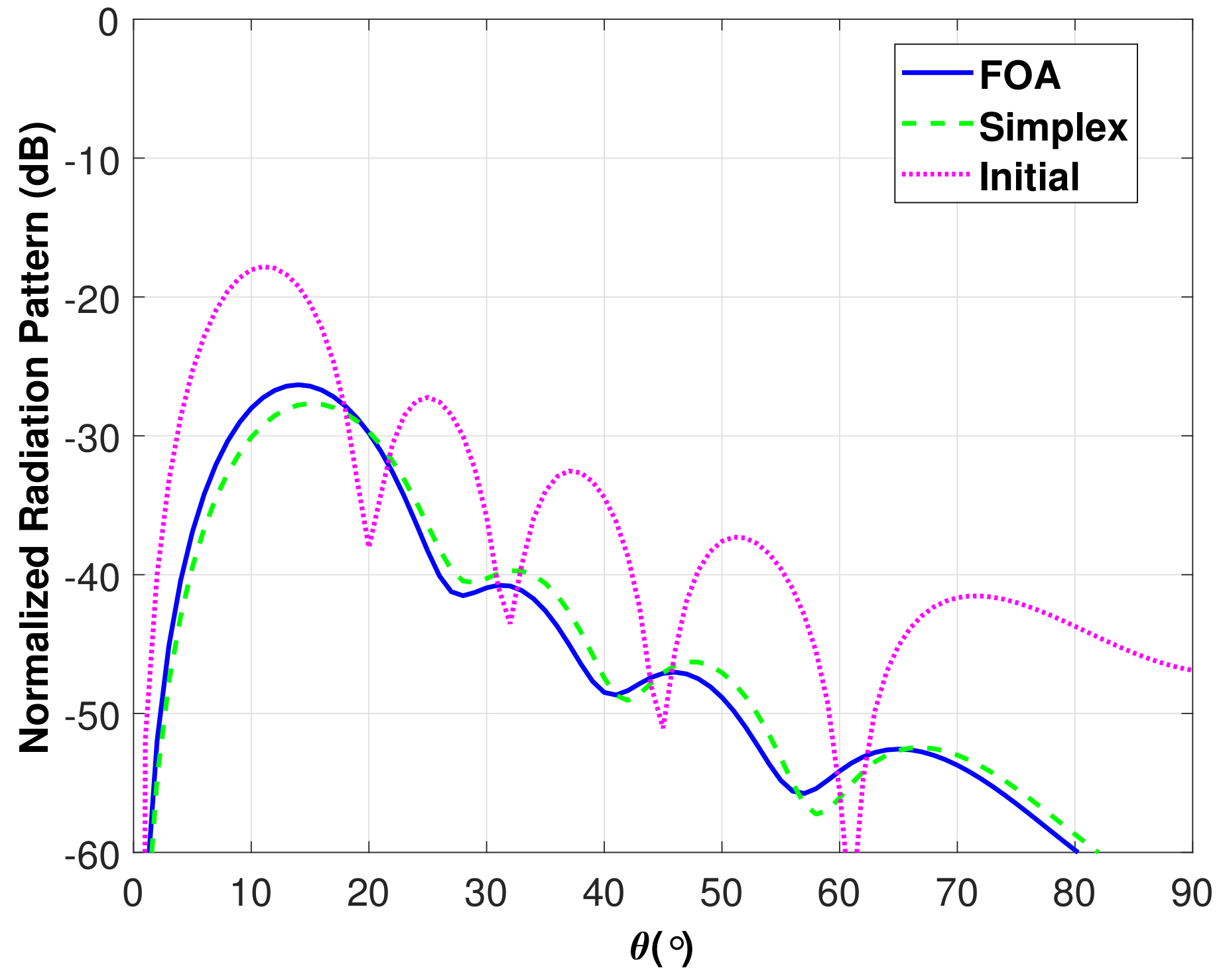
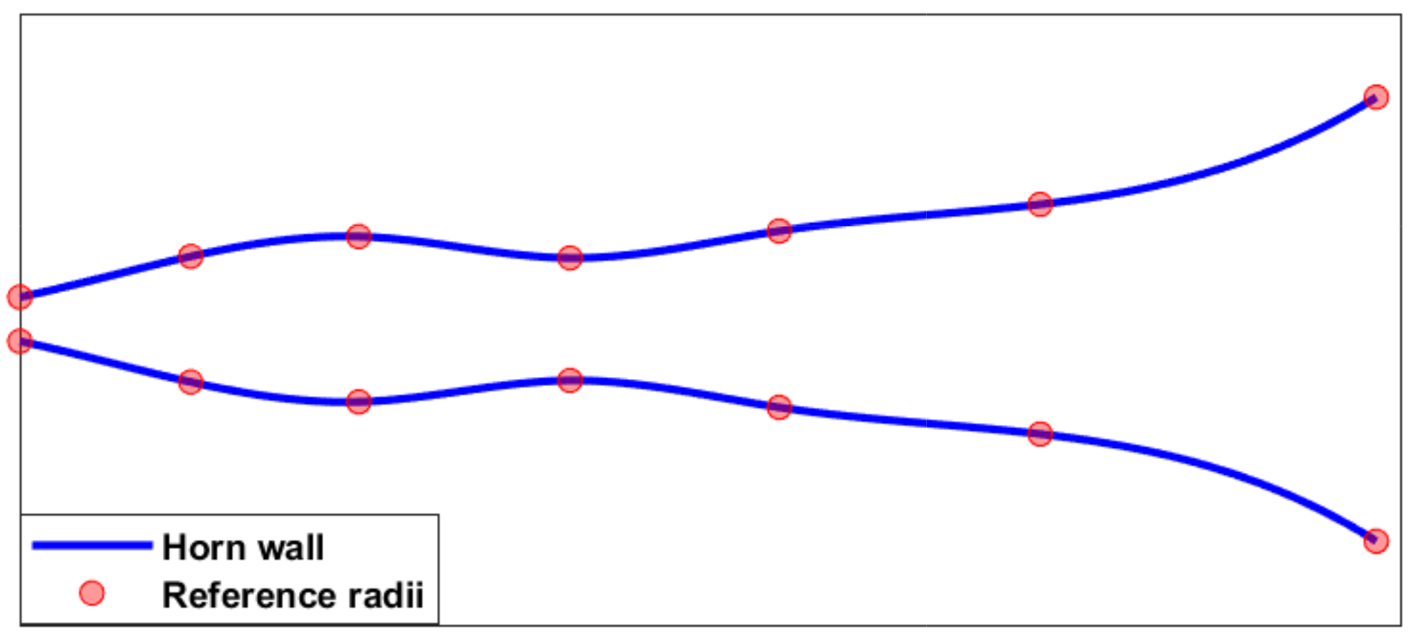
3.2. Application to Horn Antennas

To show some more complex numerical examples, in this section the FOA will be applied to the optimization of horn antennas. A horn antenna is a three-dimensional waveguide structure described by a set of geometrical parameters that can express linear or angular magnitudes (for instance, lengths of some sections, or the angle of the horn flare, respectively). The optimization of a horn consists in finding a set of these parameters that provide the best possible performance in terms of the smell function. In this case computing the smell function will require us to perform a full wave simulation of the antenna. In the present work this simulation is carried out by means of a Mode-Matching (MM) software, which provides accurate as well as fast results for these type of problems [22]. It should be noted that, to the best of the authors’ knowledge, the FOA has not previously been applied to a complex radiation problem like this.

The first optimized horn will be a Potter Horn antenna [23], which is one of the most classic, multimode horn antennas. The term “multimode horn” means that the radiation pattern is produced by a combination of modes at the horn aperture with the appropriate amplitude and phase. This modal combination lowers the SLL and the crosspolarization level with respect to the radiation pattern produced by $T{E}_{11}$ radiating aperture and also provides with a symmetric radiation pattern [23].

The profile of the horn is responsible for, starting from the fundamental mode at the horn input, generating the appropriate modal combination at the aperture. An illustration of the profile of a Potter horn antenna with its design parameters can be found in Figure 6. If the modal amplitudes are normalized to that of the fundamental mode ($T{E}_{11}$), the $T{M}_{11}$ amplitude must be $0.16$ and this mode has to be in phase with the $T{E}_{11}$, according to [23]. The amplitudes of the other modes at the aperture should be as low as possible to achieve the best results and, ideally, the return loss at the horn input should be minimized. Therefore, the employed smell function is composed of three different terms:

$$Smell={\left(\alpha ·Error\_MainModes+\beta ·Error\_HigherOrderModes+\gamma ·max\left\{\right|S_{11}\left|\right\}\right)}^{-1},$$

(7)

where $Error\_MainModes$ depends on how much the modulus and phase of the $T{M}_{11}/T{E}_{11}$ ratio differ from their desired values,

$$Error\_MainModes=\left|0.16-\frac{|Amp\_T{M}_{11}|}{|Amp\_T{E}_{11}|}\right|+|\angle T{M}_{11}-\angle T{E}_{11}|,$$

(8)

$Error\_HigherOrderModes$ consists of the sum of the amplitudes of all the modes at the aperture different from the $T{E}_{11}$ or $T{M}_{11}$,

$$Error\_HigherOrderModes=\sum |Amp\_HigherOrderModes|,$$

(9)

$S_{11}$ is the reflection coefficient of the fundamental mode at the input waveguide and $\alpha ,\beta ,\gamma$ are weighting coefficients to balance the three different terms. The modal amplitudes have to be evaluated at the design frequency which for this design will be 94 GHz.

The optimization of the parameters represented in Figure 6 must maximize the smell function in (7). The step from $r_2$ to $r_3$ is responsible for generating the $T{M}_{11}$ mode with the appropriate amplitude and, by varying the length $L_2$, the correct phasing between the two modes can be adjusted. The step between $r_1$ and $r_2$ is used just to achieve a better return loss value, since the value of $r_2$ is bounded to only allow the propagation of the fundamental mode. Finally, the flaring angle $\theta$ is chosen around ${6.5}^{\circ }$ but its final value must be optimized depending on the values chosen for the rest of the design parameters.

Since this is a well known problem there are some design formulas in the literature that can be used to obtain a first approximation of the horn profile [23]. The values provided by these formulas are used as a starting point for the optimization and can be found in

Table 3. Values of the Potter horn design parameters obtained by different methods.

Parameter	Initial	FOA	Simplex
$r_2$	1.50 mm	1.70 mm	1.64 mm
$L_2$	1.60 mm	6.11 mm	2.78 mm
$r_3$	1.95 mm	2.44 mm	2.13 mm
$L_3$	3.99 mm	2.64 mm	2.76 mm
$\theta$	${6.5}^{\circ }$	${5.29}^{\circ }$	${7.72}^{\circ }$

.

The FOA is configured to use 40 flies per swarm and to evaluate the smell function just 3000 times (this same constraint is also used for the simplex method). Additionally the maximum variation range for each parameter in a single iteration is configured as following:

• Radii: 0.15 mm
• Lengths: $0.15·{\lambda }_0$
• Angle: ${0.25}^{\circ }$

After the optimization, by means of the FOA and the simplex method, the resultant design parameters are the ones presented in Table 3. The different components of the radiation pattern can be found in Figure 7, Figure 8, Figure 9 and Figure 10. The magnitude of the $S_{11}$ parameter is represented in Figure 11.

It can be seen that the design provided by the FOA is slightly better in terms of SLL and beam symmetry, and it also presents a significantly better return loss.

The second horn that will be studied is a spline-profile horn. This is another type of multimode horn that uses a smooth varying profile (instead of using steps or corrugations) to achieve a certain mode combination at its aperture [24]. The profile of one of these antennas is defined by the spline curve that passes across a set of reference radii, as illustrated in Figure 12. Therefore by correctly varying the value of these radii the modal combination at the aperture can be adjusted.

To demonstrate that the implemented algorithm can also deal with problems that present a big number of optimization parameters, a spline-profile horn defined by 20 reference radii will be optimized. The initial values for these radii will be equispaced between the input and aperture radii value, such that the initial profile corresponds with that of a conical horn antenna. The input and aperture radii of the antenna will be 1.13 mm and 3${\lambda }_0$ = 9.57 mm, respectively. The maximum variation range for the reference radii in a single iteration will be defined to be 0.10 mm.

The same smell function used for the optimization of the Potter Horn antenna, (7), will be used in this design since it provides with a good mode combination to increase directivity and decrease the crosspolarisation level. The resultant radiation pattern after the FOA optimization can be found in Figure 13, where it can be seen that it presents a crosspolarisation level significantly lower than −20 dB and a good main beam symmetry. The $S_{11}$ is illustrated in Figure 14, revealing a value lower than −30 dB for the band of interest.

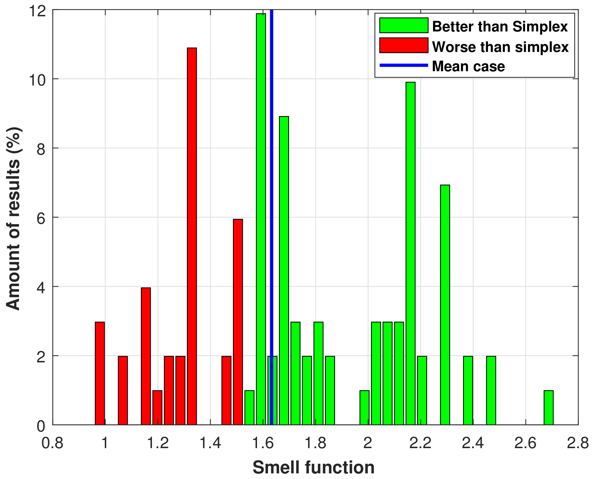
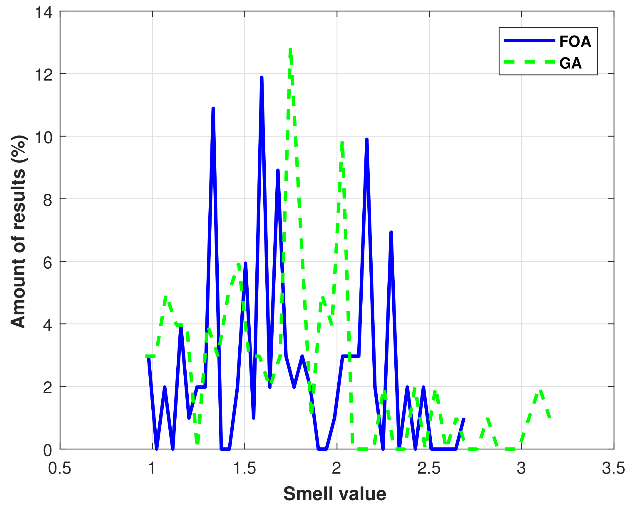
3.3. Statistical Analysis of the Results

One of the drawbacks of heuristic optimization techniques is that, because of its random nature, the results may not always be the same for different realizations. Therefore obtaining a good result for a certain optimization problem does not guarantee that the algorithm gives, in general, good results for that problem.

To asses this, a statistical study of the FOA performance has been carried out. This study consisted in performing 100 optimizations of the already presented Potter horn and then analysing the obtained smell values to compare them with the results achieved by the simplex method. In both cases (FOA and Simplex) the number of cost function evaluations has been set to 3000.

Figure 15 represents the evolution of the smell function over the FOA iterations. Three different cases are illustrated: the one that achieves the best smell function value, the one that achieves the worst and a mean of all the optimizations.

A histogram of the achieved smell function values is depicted in Figure 16. The green bars belong to the cases where the result is better than the one provided by the simplex method and the red bars belong to the cases that are worse. It can be seen that there are more cases where the result is better than that provided by simplex and therefore the mean value of the achieved smell function values (blue line) is better than the smell function value achieved by simplex.

Consequently, it can be concluded that the results provided by the FOA are, in mean, better than those achieved by the Simplex method. This shows that the FOA (as other heuristic techniques) can avoid local minima, or at least avoid them better than deterministic methods based on the derivatives of the cost function.

3.4. Comparison with a Genetic Algorithm

As a final test, results from the FOA have been compared with the ones provided by another heuristic method, the Genetic Algorithm (GA), specifically with its commercial implementation provided by Matlab [25].

The initial population of the GA has been initialized to the same value used as a starting point for the FOA optimization. Since the used implementation of the GA does not allow us to set the maximum variation range of each parameter for every single iteration, global upper/lower boundaries have been provided for the design parameters to be optimized. This is done in order to prevent the GA from achieving unrealistic values. These boundaries (presented in

Table 4. Boundaries for the design parameters during the Genetic Algorithm optimization.

Parameter	Lower Boundary	Upper Boundary
$r_2$	1.13 mm	9.57 mm
$L_2$	1.00 mm	10.00 mm
$r_3$	1.13 mm	9.57 mm
$L_3$	1.00 mm	10.00 mm
$\theta$	${2.0}^{\circ }$	${10.0}^{\circ }$

) have been chosen based on the best design provided by the FOA, with an increased interval to allow the GA to find a better maximum for the smell function.

Figure 17 shows two histograms representing the distribution of smell function values obtained by both algorithms. It can be seen that the FOA results are similar to those of the GA for the Potter Horn design. It should be borne in mind that a rigorous global comparison would require the analysis of a larger span of application problems, which is beyond the scope of this paper (focused on presenting the FOA and its application to antenna design). Overall, it can be concluded that the performance of the implemented algorithm for this problem is comparable to that of other heuristic algorithms like the commercial implementation of the GA.

4. Conclusions

In the present work an algorithm for heuristic optimization known as the Fruit fly Optimization Algorithm (FOA) has been presented. The original algorithm has been adapted for its application to two different antenna design problems: array factor synthesis and design of horn antennas.

To illustrate the usefulness of the implemented algorithm different numerical examples have been presented. The FOA has been used to synthesize two uniformly-fed, non-equispaced arrays with minimum SLL parting from an equispaced array. Additionally, two horns have been optimized with very good results. The optimization of these antennas required to perform a full wave simulation of the device (which was done using a Mode-Matching software) to compute the smell function, validating the use of this algorithm in complex electromagnetic problems..

In both cases the FOA results were compared with a deterministic optimization (based on a Simplex method), which obtained worse results since it kept getting stuck in a local minima. Finally, a small statistical study in which the FOA results were compared not only with a simplex algorithm but also with a Genetic Algorithm has been presented. All these studies show that the FOA is a very useful optimization tool for challenging antenna designs in microwave and millimetre-wave systems.

References

1. Haupt, R.L.; Menozzi, J.J.; McCormack, C.J. Thinned arrays using genetic algorithms. In Proceedings of the IEEE Antennas and Propagation Society International Symposium, Ann Arbor, MI, USA, 28 June–2 July 1993; Volume 2, pp. 712–715. [Google Scholar]
2. Johnson, J.M.; Rahmat-Samii, V. Genetic algorithms in engineering electromagnetics. IEEE Antennas Propag. Mag. 1997, 39, 7–21. [Google Scholar]
3. Ares-Pena, F.J.; Rodriguez-Gonzalez, J.A.; Villanueva-Lopez, E.; Rengarajan, S.R. Genetic algorithms in the design and optimization of antenna array patterns. IEEE Trans. Antennas Propag. 1999, 47, 506–510. [Google Scholar] [CrossRef]
4. Dey, R.; Chakrabarty, S.; Jyoti, R.; Kurian, T. Synthesis and analysis of multi-mode profile horn using mode matching technique and evolutionary algorithm. IET Microw. Antennas Propag. 2016, 10, 276–282. [Google Scholar] [CrossRef]
5. Rolland, A.; Ettorre, M.; Drissi, M.; Coq, L.L.; Sauleau, R. Optimization of Reduced-Size Smooth-Walled Conical Horns Using BoR-FDTD and Genetic Algorithm. IEEE Trans. Antennas Propag. 2010, 58, 3094–3100. [Google Scholar] [CrossRef]
6. Quevedo-Teruel, O.; Rajo-Iglesias, E. Ant Colony Optimization in Thinned Array Synthesis With Minimum Sidelobe Level. IEEE Antennas Wirel. Propag. Lett. 2006, 5, 349–352. [Google Scholar] [CrossRef]
7. Mosca, S.; Ciattaglia, M. Ant Colony Optimization to Design Thinned Arrays. In Proceedings of the 2006 IEEE Antennas and Propagation Society International Symposium, Albuquerque, NM, USA, 9–14 July 2006; pp. 4675–4678. [Google Scholar]
8. Rajo-Iglesias, E.; Quevedo-Teruel, O. Linear array synthesis using an ant-colony-optimization-based algorithm. IEEE Antennas Propag. Mag. 2007, 49, 70–79. [Google Scholar] [CrossRef]
9. Khodier, M.M.; Christodoulou, C.G. Linear array geometry synthesis with minimum sidelobe level and null control using particle swarm optimization. IEEE Trans. Antennas Propag. 2005, 53, 2674–2679. [Google Scholar] [CrossRef]
10. Donelli, M.; Martini, A.; Massa, A. A Hybrid Approach Based on PSO and Hadamard Difference Sets for the Synthesis of Square Thinned Arrays. IEEE Trans. Antennas Propag. 2009, 57, 2491–2495. [Google Scholar] [CrossRef]
11. Robinson, J.; Sinton, S.; Rahmat-Samii, Y. Particle swarm, genetic algorithm, and their hybrids: Optimization of a profiled corrugated horn antenna. In Proceedings of the IEEE Antennas and Propagation Society International Symposium (IEEE Cat. No.02CH37313), San Antonio, TX, USA, 16–21 June 2002; Volume 1, pp. 314–317. [Google Scholar]
12. Moradi, A.; Mohajeri, F. Reduction of SLL in a square horn antenna in presence of metamaterial surfaces by using of particle swarm optimization. In Proceedings of the 2016 24th Iranian Conference on Electrical Engineering (ICEE), Shiraz, Iran, 10–12 May 2016; pp. 598–603. [Google Scholar]
13. Rashedi, E.; Nezamabadi-pour, H.; Saryazdi, S. GSA: A Gravitational Search Algorithm. Inf. Sci. 2009, 179, 2232–2248. [Google Scholar]
14. Pelusi, D.; Mascella, R.; Tallini, L. Revised Gravitational Search Algorithms Based on Evolutionary-Fuzzy Systems. Algorithms 2017, 10. [Google Scholar] [CrossRef]
15. Pan, W.T. A new Fruit Fly Optimization Algorithm: Taking the financial distress model as an example. Knowl.-Based Syst. 2012, 26, 69–74. [Google Scholar] [CrossRef]
16. Liu, Y.; Wang, X.; Li, Y. A Modified Fruit-Fly Optimization Algorithm aided PID controller designing. In Proceedings of the 10th World Congress on Intelligent Control and Automation, Beijing, China, 6–8 July 2012; pp. 233–238. [Google Scholar]
17. Li, H.Z.; Guo, S.; Li, C.J.; Sun, J.Q. A hybrid annual power load forecasting model based on generalized regression neural network with fruit fly optimization algorithm. Knowl.-Based Syst. 2013, 37, 378–387. [Google Scholar] [CrossRef]
18. Mhudtongon, N.; Phongcharoenpanich, C.; Kawdungta, S. Modified Fruit Fly Optimization Algorithm for Analysis of Large Antenna Array. Int. J. Antennas Propag. 2015, 2015, 124675. [Google Scholar] [CrossRef]
19. Mhudtongon, N.; Phongcharoenpanich, C.; Watanabe, K. Linear antenna synthesis with maximum directivity using improved fruit fly optimization algorithm. In Proceedings of the 2016 URSI International Symposium on Electromagnetic Theory (EMTS), Espoo, Finland, 14–18 August 2016; pp. 698–701. [Google Scholar]
20. Pan, W.T. Fruit Fly Optimization Algorithm (Using MATLAB). 2014. Available online: https://www.mathworks.com/matlabcentral/answers/uploaded_files/20100/Fruit%20Fly%20Optimization%20Algorithm_Second%20Edition.pdf (accessed on 1 February 2014).
21. Stutzman, W.L.; Thiele, G. Antenna Theory and Design; John Wiley & Sons: Hoboken, NJ, USA, 1998. [Google Scholar]
22. Conciauro, G.; Guglielmi, M.; Sorrentino, R. Advanced Modal Analysis: CAD Techniques for Waveguide Components and Filters; John Wiley & Sons: Hoboken, NJ, USA, 2000. [Google Scholar]
23. Olver, A.; Clarricoats, P.; Kishk, A.; Shafai, L. Microwave Horns and Feeds; Electromagnetic Waves Series; IEE: London, UK; IEEE: New York, NY, USA, 1994. [Google Scholar]
24. Granet, C.; James, G.L.; Bolton, R.; Moorey, G. A smooth-walled spline-profile horn as an alternative to the corrugated horn for wide band millimeter-wave applications. IEEE Trans. Antennas Propag. 2004, 52, 848–854. [Google Scholar] [CrossRef]
25. MATLAB R2016b; The MathWorks, Inc.: Natick, MA, USA, 2017.
Figure 1. Schematic representation of the FOA behaviour.
Electronics 07 00003 g001
Figure 2. Schematic representation of the linear array.
Electronics 07 00003 g002
Figure 3. Representation of the spherical coordinate system used in this work.
Electronics 07 00003 g003
Figure 4. Array factor of the first example.
Electronics 07 00003 g004
Figure 5. Array factor of the second example.
Electronics 07 00003 g005
Figure 6. Representation of the Potter horn profile.
Electronics 07 00003 g006
Figure 7. Normalized radiation pattern at 94 GHz of the of the optimized Potter Horn (H-Plane).
Electronics 07 00003 g007
Figure 8. Normalized radiation pattern at 94 GHz of the of the optimized Potter Horn (E-Plane).
Electronics 07 00003 g008
Figure 9. Normalized radiation pattern at 94 GHz of the of the optimized Potter Horn (Diagonal Plane, Copolar Component).
Electronics 07 00003 g009
Figure 10. Normalized radiation pattern at 94 GHz of the of the optimized Potter Horn (Diagonal Plane, Crosspolar Component).
Electronics 07 00003 g010
Figure 11. Magnitude of the S 11 parameter of the optimized Potter Horn.
Electronics 07 00003 g011
Figure 12. Representation of a spline-profile horn.
Electronics 07 00003 g012
Figure 13. Normalized radiation pattern at 94 GHz of the of the optimized spline-profile horn.
Electronics 07 00003 g013
Figure 14. Magnitude of the S 11 parameter of the optimized spline-profile horn.
Electronics 07 00003 g014
Figure 15. Evolution of the smell function value over the iterations of the statistical study.
Electronics 07 00003 g015
Figure 16. Histogram of the smell function values achieved during the statistical study.
Electronics 07 00003 g016
Figure 17. Comparison of the results provided by the implemented FOA and a commercial implementation of a GA. S m e l l ¯ F O A = 1.73, σ F O A = 0.41, S m e l l ¯ G A = 1.71, σ G A = 0.49. Mean value ( S m e l l ¯ x ) and variance ( σ x ) of the Smell function results.
Electronics 07 00003 g017