Hierarchical Consistency-Based Cooperative Control Strategy Integrating Load-Observation-Based Dynamic Feedforward and Adaptive Particle Swarm Optimization

Abstract

In the parallel operation of islanded microgrids, line impedance mismatches and random load fluctuations, along with the dynamic response lag and difficulty in multidimensional parameter tuning of traditional control strategies, lead to power sharing imbalances and instability in frequency and voltage. To address these issues, this paper proposes a hierarchical cooperative control strategy based on consistency that integrates load-observation-based dynamic reference feedforward (LODRF) and adaptive particle swarm optimization (APSO). First, an improved adaptive virtual impedance (IAVI) strategy based on consistency is introduced into the virtual synchronous generator control framework. Second, an LODRF mechanism is applied at the secondary control layer to actively reconstruct the power baseline by observing the load status at the point of common coupling (PCC) in real time. Furthermore, an APSO algorithm utilizing the integral of time-weighted absolute error (ITAE) as a global performance index is constructed to optimize key proportional–integral controller parameters cooperatively. Simulation results from a four-unit heterogeneous parallel system in MATLAB/Simulink demonstrate that the IAVI strategy enables stable convergence of frequency and voltage and proportional power sharing. Compared with the system without LODRF, the proposed strategy reduces maximum frequency and voltage dynamic deviations under load disturbances by 78.5% and 53.3%, respectively, and shortens effective recovery times by 0.01 s and 0.09 s, respectively. Moreover, compared with the standard PSO algorithm, the APSO-optimized system reduces maximum frequency and voltage deviations by 3.1% and 36.4%, respectively. Additionally, average active and reactive power sharing errors in the steady state are kept below 0.9%, verifying the significant advantages of the strategy in improving dynamic disturbance rejection and steady-state precision.

1. Introduction

In the context of the accelerating global energy transition and the deepening implementation of the “dual carbon” strategy, the penetration rate of distributed generation (DG), represented by wind and photovoltaic (PV) power, continues to rise in power systems. This has made microgrid technology a key carrier for the flexible consumption of distributed energy and efficient grid management [1,2]. Microgrids operate in two modes: grid-connected and islanded, with stable operation under islanded mode being particularly critical [3]. When a microgrid disconnects from the main grid and enters islanded operation, the system loses the rigid voltage and frequency support provided by the large grid. Consequently, it becomes highly susceptible to random load fluctuations, intermittent output changes from renewable energy sources, and network topology switching, facing severe challenges such as uneven power sharing and dynamic instability of voltage and frequency [4]. To address the issues of low inertia and weak damping characterizing high-penetration power-electronic-based power systems, virtual synchronous generator (VSG) control technology has emerged as a solution [5]. By simulating the rotor motion equations and electromagnetic transient characteristics of synchronous generators in the inverter control loop, VSG provides necessary inertia support and damping, becoming a mainstream control scheme for enhancing frequency and voltage stability in islanded microgrids [6,7].

However, traditional VSG control essentially relies on active power–frequency (P-f) and reactive power–voltage (Q-V) droop characteristics to achieve multi-unit parallel operation [8]. Although this mechanism facilitates autonomous power sharing, it introduces unavoidable inherent limitations when confronting load fluctuations and non-homogeneous physical networks. On the one hand, traditional droop control relies on a passive error-accumulation mechanism to respond to load variations. When an islanded microgrid is subjected to sudden load fluctuations, this passive response mechanism struggles to rapidly establish a new power equilibrium. Consequently, the system becomes highly susceptible to severe dynamic frequency and voltage dips, or even transient instability, thereby degrading the overall power quality [9]. On the other hand, in low-voltage microgrids, line impedances typically exhibit resistive-inductive characteristics, and their parameters often display significant spatial disparities due to varying physical locations. Such non-homogeneous line impedances directly result in mismatched equivalent output impedances among DG units, thereby invalidating the power decoupling assumptions underlying traditional P-f and Q-V droop controls. The resultant active-reactive power coupling not only impedes the precise sharing of reactive power proportional to DG capacities but also triggers high-frequency oscillations and severe reactive circulating currents among parallel inverters [10], which severely compromise the operational security and equipment reliability of the microgrid [11]. To overcome the limitations of primary control, existing research widely adopts a hierarchical control architecture, introducing a secondary control layer to achieve zero-error recovery of frequency and voltage, as well as precise power sharing. Early secondary control mostly adopted a centralized architecture, which relies heavily on a central controller and high-bandwidth communication, posing a risk of single-point failure [12,13].

Compared with centralized schemes, distributed control strategies utilize sparse communication networks, offering advantages such as strong robustness, low communication costs, high reliability, and ease of system expansion. Reference [14] added an integral feedforward compensation loop to distributed secondary control, achieving frequency difference elimination between inverters without communication. Reference [15] added a secondary frequency regulation strategy to the droop control, allowing frequency to autonomously recover to nominal values in standalone microgrids, but neither considered the restoration of reactive power and voltage. Reference [16] proposed an improved Q-V droop control strategy that effectively improved voltage control precision, yet the system voltage could not be accurately restored to the nominal value. Reference [17] applied virtual impedance technology and fractional-order PI controllers to secondary frequency regulation; however, focusing primarily on local circuit topology control without distributed multi-unit coordination, it is rendered inadequate for complex microgrids featuring heterogeneous impedances. Reference [18] presents a decentralized adaptive virtual impedance framework that dynamically modulates virtual impedance utilizing local output currents to facilitate accurate power sharing. To augment dynamic stability, the authors in [19] leverage a model based on small signal analysis to execute the offline parameter tuning of both droop and dual closed-loop controllers via a hybrid optimization algorithm. Nevertheless, the scope of these methodologies remains strictly restricted to the primary control stratum. As a result, they possess an inherent inability to eradicate the deviations intrinsic to conventional droop mechanisms in the steady state, failing to accomplish the exact secondary restoration of system frequency and voltage. In recent years, consensus algorithms based on multi-agent systems (MASs) have become a research hotspot in distributed secondary control due to their decentralization and strong robustness. Reference [20] realized secondary voltage recovery and load redistribution based on MAS distributed control. Reference [21] proposed a distributed cooperative control strategy combining MAS consensus algorithms, achieving precise power sharing and effectively suppressing circulating currents. Although the above methods considered consensus-based droop control, they did not utilize it for the adaptive regulation of virtual impedance. References [22,23] adopted event-triggered mechanisms in distributed consensus secondary control, effectively reducing the microgrid’s dependence on communication networks while maintaining high regulation precision. However, multi-objective coordination under secondary control was not realized.

Furthermore, with the introduction of secondary control, the microgrid control system evolves into a high-order, nonlinear, and strongly coupled complex system, involving the cooperative tuning of VSG primary control parameters and secondary control gains. To solve the difficulty of parameter tuning, intelligent optimization algorithms have been introduced. References [24,25] used deep reinforcement learning (DRL) to realize distributed frequency regulation, but this requires pre-training and necessitates retraining when model generalization ability is weak. References [26,27] applied particle swarm optimization (PSO) to the parameter optimization of droop control, effectively improving power coupling and sharing precision, but they failed to eliminate static errors in frequency and voltage caused by load changes. Reference [28] utilized the PSO algorithm to solve convergence issues in complex microgrid power flow calculations; however, it focused primarily on steady-state economic operation or static analysis, and the weights in the fitness function were fixed. Reference [29] proposed a multi-VSG reactive power sharing and voltage support control based on twin delayed deep deterministic policy gradient (TD3) but ignored frequency support issues. Reference [30] proposed a dynamic inertia VSG control based on MAS and DRL, effectively suppressing system power oscillations, yet it failed to consider power sharing. Reference [31] proposed a multi-objective parameter optimization framework based on the PSO algorithm, achieving global optimization of control parameters and smooth switching between modes by simultaneously optimizing key pole damping in grid-connected and islanded modes; however, it lacked the capability for online adaptive adjustment.

Existing research has extensively explored dynamic disturbance rejection in microgrids. Specifically, Reference [32] developed a synchronization strategy utilizing self-recovery droop control to maintain frequency stability during mode transitions. Reference [33] suppressed harmonic interference caused by nonlinear loads utilizing grid-side voltage feedforward compensation, while the frequency self-recovery trajectory was optimized in reference [34] by introducing deviation-proportional feedforward. Although these localized methods achieve effectiveness, control strategies remain predominantly focused on the elimination of steady-state errors in frequency and voltage. In view of the deficiencies in active load disturbance rejection and global cooperative optimization of control parameters in existing research, this paper proposes a consistency-based hierarchical cooperative control strategy for islanded microgrids that integrates load-observation-based dynamic reference feedforward (LODRF) and adaptive particle swarm optimization (APSO). The main contributions and structure of this paper are summarized as follows:

(1)

An improved adaptive virtual impedance (IAVI) strategy is proposed to establish coordination between the primary and secondary control layers. By incorporating consistency error signals from the secondary layer to reconfigure virtual parameters, this method compensates for voltage drop differences caused by line impedance mismatches and improves power decoupling.

(2)

An active feedforward control mechanism based on LODRF is proposed. By observing load power variations at the point of common coupling (PCC) in real time, a feedforward path is established to reconstruct the power baseline for each VSG unit. This strategy overcomes the inherent response latency of feedback control, significantly reducing the transient excursions of frequency and voltage while accelerating the dynamic recovery process.

(3)

An optimization model based on the APSO algorithm is established using the integral of time-weighted absolute error (ITAE) as the objective function. This approach incorporates voltage and current dual-loop control parameters into a unified optimization space, resulting in smoother waveforms after optimization compared to the standard PSO (SPSO) algorithm.

(4)

A simulation model of an islanded microgrid containing four heterogeneous distributed generation units is established. Under scenarios of sudden load increase and decrease, comparison of the system before and after adding the IAVI and LODRF modules, as well as with different PSO models, verifies the significant advantages of the proposed strategy over traditional strategies in terms of error recovery of frequency and voltage and precise power sharing.

2. Basic Principles of VSG Primary Control

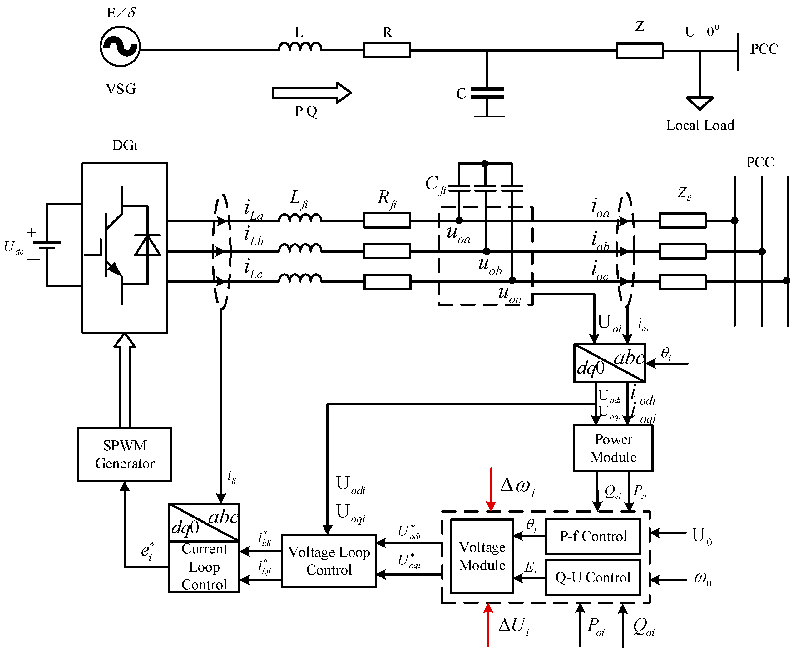
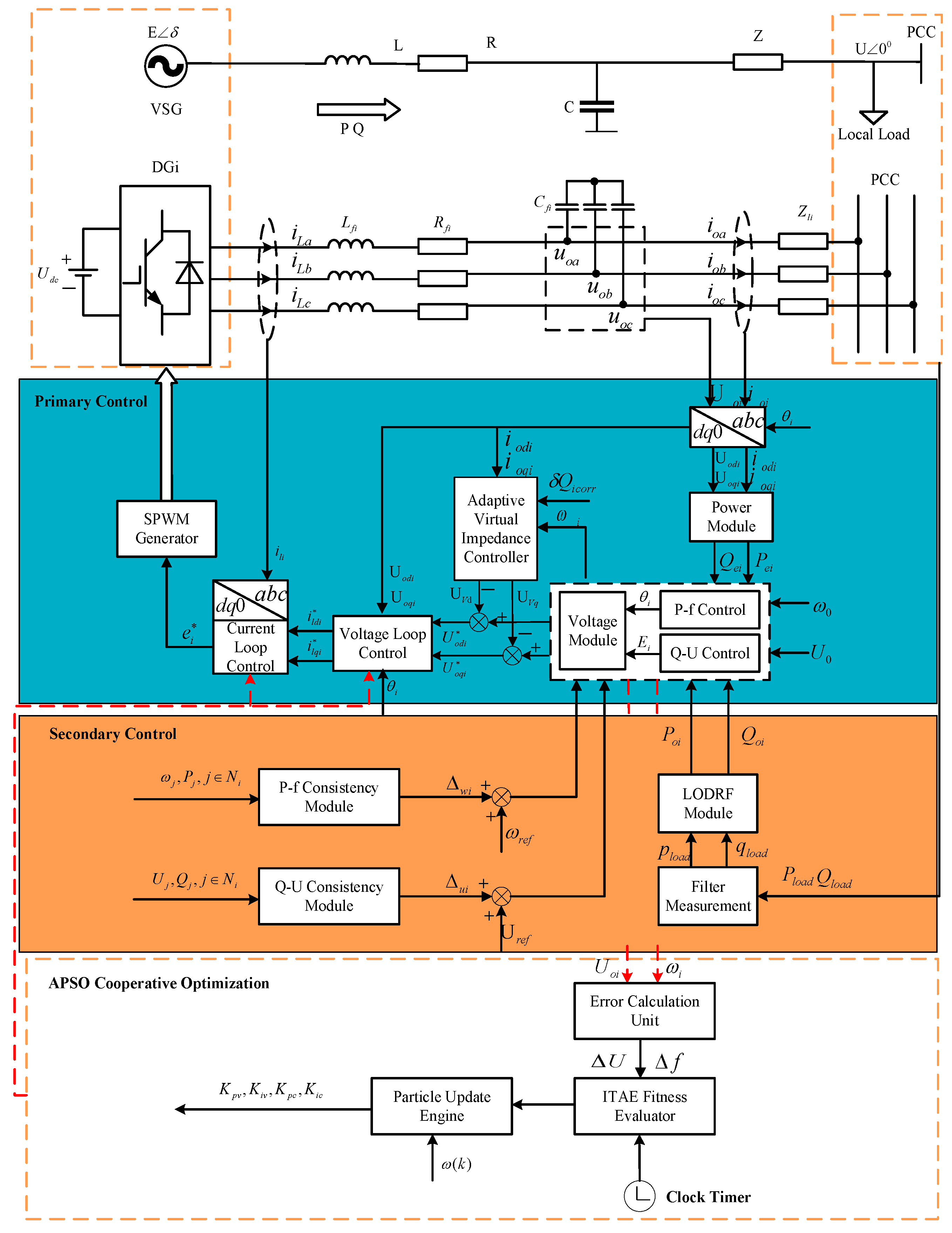
The control system proposed in this paper adopts a hierarchical architecture, comprising a primary control layer and a secondary control layer. The structure of the primary control is shown in Figure 1.

At the primary control layer, each single DG unit contains the main VSG control, which consists of the power calculation module, droop control, and the voltage and current dual-loop control module. Specifically, voltage and current sensors transmit the measured three-phase load voltage and current to the instantaneous power calculation module to obtain the active and reactive power output of the system. After filtering, these values are fed into the active power–frequency regulator and the reactive power–voltage exciter, respectively, to generate the required reference phase angle and reference voltage. Finally, these references are synthesized and input into the voltage and current dual-loop control module to generate the modulation wave, thereby controlling the switching of the six IGBTs in the three-phase inverter bridge, completing the basic VSG control process.

2.1. VSG Droop Control System

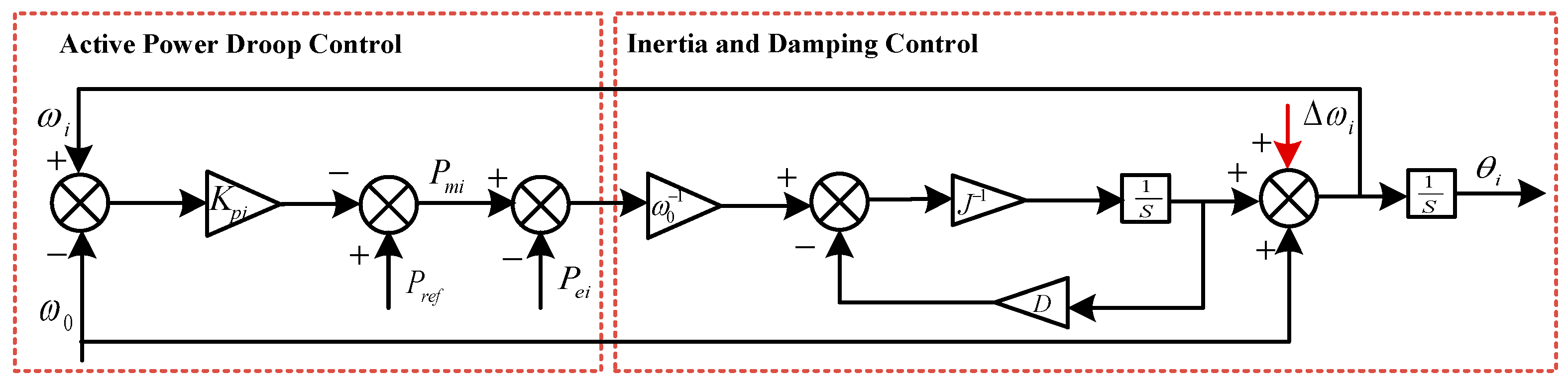
In SGs, primary frequency regulation is achieved by the governor, which functions to modulate the mechanical power output of the prime mover in response to variations in grid frequency. The governor module of the VSG can be designed by emulating the variation relationship between the active power and frequency of the SG. The mechanical power $P_m$ based on the droop characteristic is defined as

$$P_m=P_{ref}-K_p(\omega -{\omega }_0)$$

(1)

where $P_{ref}$ denotes the active power reference value, and $K_p$ represents the active power droop coefficient.

The motion of a synchronous generator’s rotor is governed by Newton’s second law, which establishes the physical relationship between unbalanced power and the rate of change in frequency:

$$\left\{\begin{array}{l}J{\displaystyle \frac{d\Delta \omega }{dt}}=T_m-T_e-T_d={\displaystyle \frac{P_m}{{\omega }_0}}-{\displaystyle \frac{P_e}{{\omega }_0}}-D\Delta \omega \\ \Delta \omega =\omega -{\omega }_0\\ {\displaystyle \frac{d\theta }{dt}}=\omega \end{array}\right.$$

(2)

where $J, D$ represent the moment of inertia and the damping coefficient, respectively; ${T_m, T}_e$ and $T_d$ denote the mechanical torque, electromagnetic torque, and damping torque of the synchronous generator, respectively; $P_m$,$P_e$ refer to the virtual mechanical input power and output electromagnetic power, respectively; $\omega , {\omega }_0$ signify the actual angular velocity and nominal angular velocity, respectively; and $\theta$ is defined as the power angle.

By substituting Equation (1) into Equation (2) and rearranging the terms, the closed-loop dynamic equation for the active power loop of the VSG is obtained:

$$J{\omega }_0{\displaystyle \frac{d\omega }{dt}}+(D{\omega }_0+K_p)(\omega -{\omega }_0)=P_{ref}-P_e$$

(3)

A typical first-order inertial element is characterized by Equation (3). The condition ${\displaystyle \frac{d\omega }{dt}}=0$ is satisfied when the system reaches the steady state. At this juncture, the frequency deviation $\Delta \omega =\omega -{\omega }_0$ is directly proportional to the power deviation $\Delta P=P_{ref}-P_e$, and the accuracy of active power sharing among parallel units is determined by $K_p$. The time constant is expressed as $\tau \approx {\displaystyle \frac{J{\omega }_0}{D{\omega }_0+K_p}}$. The time constant is increased by a larger inertia $J$, resulting in a slower rate of frequency change, thereby enhancing the disturbance rejection capability of the system against transient fluctuations.

Consequently, the emulation of the active power–frequency regulation characteristic of the SG within the VSG is illustrated in Figure 2.

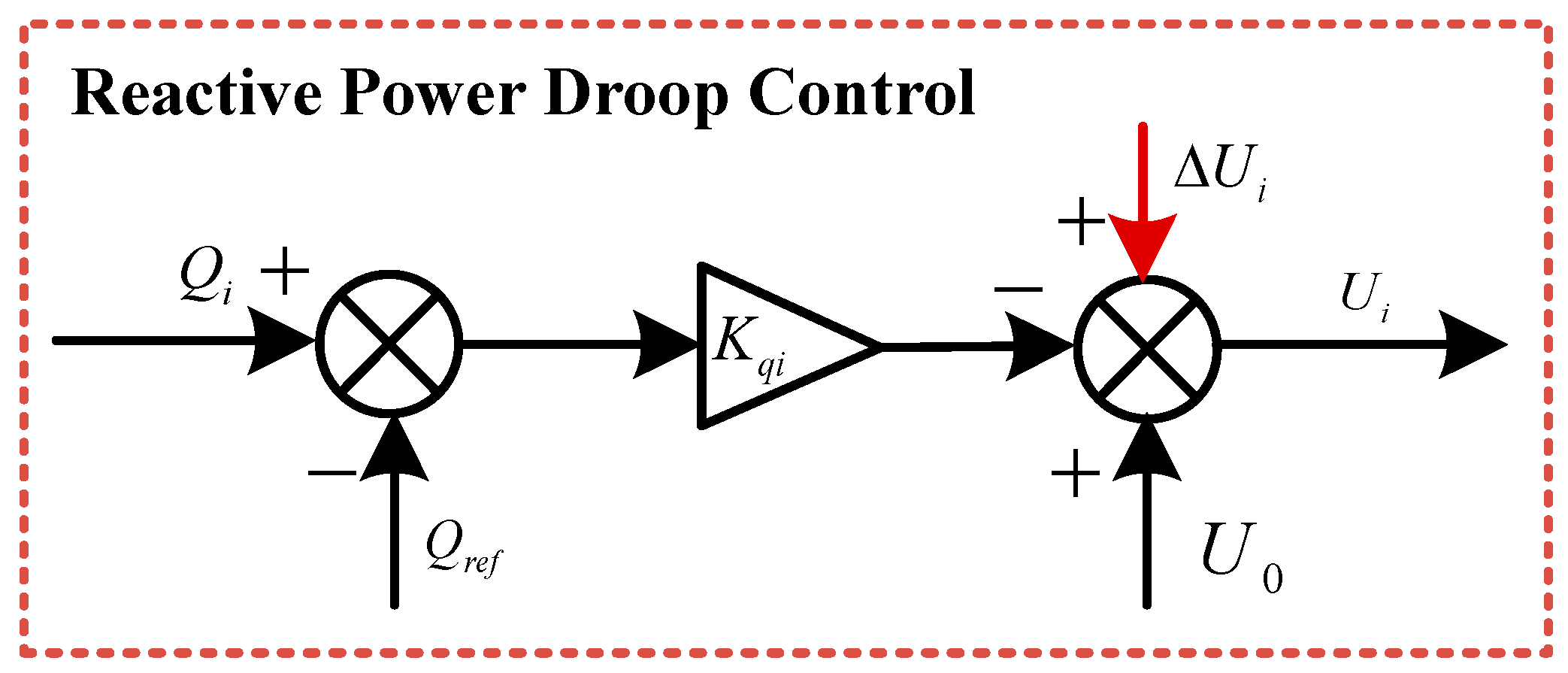
The automatic voltage regulator (AVR) functions to maintain the stability of the terminal voltage by regulating the rotor excitation current in real time to control the internal induced electromotive force. In islanded microgrids, the VSG control strategy emulates the regulation characteristics of the AVR by introducing a reactive Q-V droop mechanism. This mechanism dynamically adjusts the output voltage amplitude of the inverter according to the reactive power demand of the system, thereby achieving voltage support and rational reactive load sharing among multiple DG units.

To emulate the excitation characteristics based on the Q-V droop control strategy, the control law is expressed as

$$U=U_0-K_q(Q-Q_{ref})$$

(4)

where $U$ denotes the internal reference voltage amplitude of the VSG; $U_0$ represents the no-load nominal voltage amplitude; $Q$ signifies the measured output reactive power; $Q_{ref}$ refers to the reactive power reference value; and $K_q$ is defined as the reactive droop coefficient.

The specific implementation of the reactive power–voltage regulation is depicted in Figure 3. As illustrated, the control loop dynamically synthesizes the output voltage reference $E$ based on Equation (4). According to this control logic, when the system’s reactive power $Q$ increases, the inverter automatically reduces the output voltage amplitude $E$ according to $K_q$, thereby altering the voltage drop distribution across the output impedance. For parallel inverters with similar impedance characteristics, this mechanism ensures that reactive power is precisely shared in inverse proportion to the droop coefficients.

2.2. Voltage and Current Dual Closed-Loop System

The internal reference voltage amplitude U and phase angle $\theta$ are derived from the aforementioned control strategies. However, direct utilization of these signals as modulation waves for sinusoidal pulse width modulation (SPWM) would render the system open-loop, resulting in high sensitivity to load disturbances and susceptibility to LC filter resonance. Consequently, to ensure high-quality output voltage waveforms and rapid dynamic tracking capabilities, a voltage and current dual-loop control architecture is established beneath the power outer loop.

Governed by KVL and Kirchhoff’s current law (KCL), the dynamic balance equations of the circuit in the three-phase stationary coordinate system can be formulated as

$$\left\{\begin{array}{c}{L}_f{\displaystyle \frac{d{i}_{La}}{dt}}=u_{La}-u_{oa}-R_f{i}_{La}\\ L_f{\displaystyle \frac{d{i}_{Lb}}{dt}}=u_{Lb}-u_{ob}-R_f{i}_{Lb}\\ L_f{\displaystyle \frac{d{i}_{Lc}}{dt}}=u_{Lc}-u_{oc}-R_f{i}_{Lc}\end{array}\right.$$

(5)

$$\left\{\begin{array}{c}{C}_f{\displaystyle \frac{d{u}_{oa}}{dt}}=i_{La}-i_{oa}\\ C_f{\displaystyle \frac{d{u}_{ob}}{dt}}=i_{Lb}-i_{ob}\\ C_f{\displaystyle \frac{d{u}_{oc}}{dt}}=i_{Lc}-i_{oc}\end{array}\right.$$

(6)

where $u_{La,b,c}$ and $u_{oa,b,c}$ denote the three-phase output voltages of the inverter bridge arms and the filter capacitor voltages, respectively; $i_{La,b,c}$ and $i_{oa,b,c}$ represent the currents flowing through the filter inductor $L_f$ and the output currents flowing to the load, respectively; and $C_f,R_f$ signify the filter capacitance, and parasitic resistance of the inductor, respectively.

By applying the Park transformation, the mathematical model of the inverter main circuit in the synchronous rotating $dq$ coordinate system is derived as

$$\left\{\begin{array}{c}{L}_f{\displaystyle \frac{d{i}_{Ld}}{dt}}=u_{Ld}-u_{od}+\omega L_f{i}_{Lq}-R_f{i}_{Ld}\\ L_f{\displaystyle \frac{d{i}_{Lq}}{dt}}=u_{Lq}-u_{oq}-\omega L_f{i}_{Ld}-R_f{i}_{Lq}\end{array}\right.$$

(7)

$$\left\{\begin{array}{c}{C}_f{\displaystyle \frac{d{u}_{od}}{dt}}=i_{Ld}-i_{od}+\omega C_f{u}_{oq}\\ C_f{\displaystyle \frac{d{u}_{oq}}{dt}}=i_{Lq}-i_{oq}-\omega C_f{u}_{od}\end{array}\right.$$

(8)

where subscripts $d$ and $q$ denote the components on the d-axis and q-axis, respectively.

It is evident from Equations (7) and (8) that cross-coupling terms exist between the variables of the two axes, which severely degrades the system’s dynamic performance. To achieve independent decoupled control, PI controllers incorporating feedforward compensation are adopted.

The objective of the inner current loop is to rapidly track the current command and enhance system bandwidth. Let $u_{Ld}^{\ast }$ and $u_{Lq}^{\ast }$ be the inverter output voltage commands. The control law is designed as

$$\left\{\begin{array}{c}{u}_{Ld}^{\ast }=K_{pc}(i_{Ld}^{\ast }-i_{Ld})+K_{ic}\int (i_{Ld}^{\ast }-i_{Ld})dt-\omega L_f{i}_{Lq}+u_{od}\\ u_{Lq}^{\ast }=K_{pc}(i_{Lq}^{\ast }-i_{Lq})+K_{ic}\int (i_{Lq}^{\ast }-i_{Lq})dt+\omega L_f{i}_{Ld}+u_{oq}\end{array}\right.$$

(9)

where $K_{pc}$ and $K_{ic}$ are the PI parameters of the current loop; and $i_{Ld}^{\ast }$, $i_{Lq}^{\ast }$ are the inverter output current commands. By introducing the cross-coupling feedforward compensation terms ($\omega L_f{i}_{Lq}, \omega L_f{i}_{Ld}$) and voltage feedforward terms ($u_{oq}$, $u_{oq}$), the physical coupling within the system is mathematically neutralized, thereby simplifying the closed-loop transfer function into a first-order system.

The outer voltage loop is designed to track the voltage reference $U$ generated by the VSG and provide the current reference $i_L^{\ast }$ for the inner loop. Its control law is expressed as

$$\left\{\begin{array}{c}{i}_{Ld}^{\ast }=K_{pv}(u_{od}^{\ast }-u_{od})+K_{iv}\int (u_{od}^{\ast }-u_{od})dt-\omega C_f{u}_{oq}+i_{od}\\ i_{Lq}^{\ast }=K_{pv}(u_{oq}^{\ast }-u_{oq})+K_{iv}\int (u_{oq}^{\ast }-u_{oq})dt+\omega C_f{u}_{od}+i_{oq}\end{array}\right.$$

(10)

where $K_{pv}$ and $K_{iv}$ are the PI parameters of the voltage loop; and $u_{od}^{\ast }$, $u_{oq}^{\ast }$ are the filter output voltage commands. The introduction of cross-coupling terms ($\omega C_f{u}_{oq}$, $\omega C_f{u}_{od}$) and load current feedforward ($i_{oq}$, $i_{oq}$) significantly improves the dynamic response speed under sudden load variations and mitigates voltage dips.

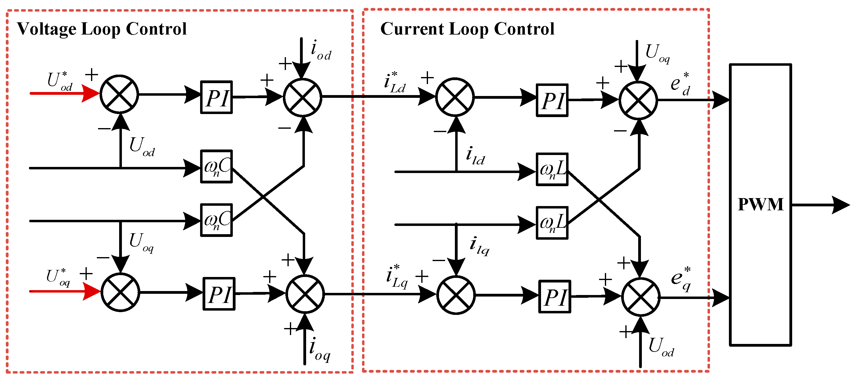
The schematic of the VSG voltage and current dual-loop control is depicted in Figure 4. Through dual PI controllers and feedforward decoupling, independent control of the dq-axis currents and voltages is realized, ensuring excellent steady-state tracking performance.

3. Distributed Secondary Cooperative Control Strategy

While primary control realizes the fundamental functionality of the VSG, the inherent characteristics of droop control inevitably result in steady-state deviations in system frequency and voltage. Furthermore, line impedance mismatches among distributed generation units hinder precise power sharing. Consequently, a secondary control layer is introduced to eliminate steady-state errors and achieve zero-error recovery of frequency and voltage, along with accurate power allocation. The distributed cooperative control architecture adopted is depicted in Figure 5.

The secondary control framework is illustrated in Figure 5, the load feedforward module utilizes measurements from the PCC to generate dynamic power references, P* and Q*, after filtering. These references are employed to modify the static power setpoints of the primary control. Simultaneously, distributed secondary controllers cooperatively compute frequency and voltage feedback compensation signals, $\Delta {\omega }_i$ and $\Delta U_i$, via a consensus algorithm over a sparse communication network. Each VSG unit exchanges information solely with its neighboring nodes. By generating compensation signals through consistency protocols, the strategy eliminates steady-state deviations under load disturbances, realizing zero-error restoration of frequency and voltage while ensuring that active and reactive power are shared precisely in proportion to the rated capacities of the DGs.

The evolution of control parameters toward the global optimum is driven by the APSO cooperative optimization layer through a closed-loop iterative mechanism, where the PI coefficients of the voltage and current loops are defined as the initial particle swarm within a four-dimensional search space. Within each iteration cycle, nonlinear inertia weights are dynamically adjusted as a function of the current iteration count to maintain an optimal balance between global exploration breadth and local convergence precision. Subsequently, the transient trajectories of frequency and voltage under load perturbations are captured in real time by the ITAE fitness evaluation unit, with the resulting time-weighted absolute error integral being utilized for particle parameter updates. By evaluating individual historical experiences ($P_{\mathit{best}}$) against the global swarm optimum ($G_{\mathit{best}}$), the velocity and position of each particle are collaboratively corrected. This optimization process is executed iteratively until the system performance index converges to a predefined threshold. Consequently, a set of optimal control parameters is generated to ensure rapid transient recovery and high steady-state precision across various disturbance conditions, thereby realizing a deep functional synergy between the underlying physical control and the intelligent optimization algorithm.

3.1. Load-Observation-Based Dynamic Reference Feedforward Strategy

In traditional droop control, power reference values are typically fixed at nominal operating points. Under this static reference paradigm, the controller responds passively to total system load variations, relying on the accumulation of local power errors. This mechanism suffers from inherent drawbacks, including dynamic response lag and significant transient power sharing deviations. The core philosophy of the LODRF strategy is to leverage real-time load information from the PCC to actively update the power baseline of each VSG, thereby enhancing the system’s dynamic disturbance rejection capability.

The total active power $P_{load}\left(t\right)$ and reactive power ${\mathrm{Q}}_{load}\left(t\right)$ on the system side are acquired at the PCC. To mitigate measurement noise and high-frequency harmonics induced by inverter switching, the acquired signals undergo low-pass filtering:

$$\left\{\begin{array}{c}{P}_{load}^{avg}(t)={\displaystyle \frac{{\omega }_c}{s+{\omega }_c}}{P}_{load}(t)\\ {\mathrm{Q}}_{load}^{avg}(t)={\displaystyle \frac{{\omega }_c}{s+{\omega }_c}}{\mathrm{Q}}_{load}(t)\end{array}\right.$$

(11)

where ${\omega }_{\mathrm{c}}$ denotes the cut-off frequency of the low-pass filter (typically set to 100 rad/s); and ${ P}_{load}^{avg}$, ${\mathrm{Q}}_{load}^{avg}$ represent the smoothed total load observations.

Assuming the system comprises $N$ DG units and the rated apparent capacity of the $i$-th DG is $S_{n,i}$, the power sharing weight coefficient $k_i$ is defined as

$$k_i={\displaystyle \frac{S_{n,i}}{\sum _{j=1}^N{S}_{n,j}}}$$

(12)

It is evident from Equation (12) that ${\sum }_{i=1}^N{k}_i=1$. According to the LODRF strategy, the power reference value for the $i$-th DG is formulated as

$$\left\{\begin{array}{c}{P}_{0,i}\left(t\right)=k_i\cdot P_{load}^{avg}\left(t\right)\\ Q_{0,i}\left(t\right)=k_i\cdot {\mathrm{Q}}_{load}^{avg}\left(t\right)\end{array}\right.$$

(13)

Upon a step change in load, each DG can directly acquire the target power reference allocated based on capacity ratios, bypassing the delay associated with error accumulation. This mechanism effectively accelerates the transient response speed of the system.

3.2. Consistency-Based Frequency Restoration and Active Power Sharing

To restore the system frequency to its nominal value ${\omega }_0$ and ensure active power is shared precisely according to capacity, a frequency-active power secondary controller is designed as follows:

$$\left\{\begin{array}{c}\Delta {\dot{\omega }}_i=-c_{\omega }{\sum }_{j\in N_i}{a}_{ij}\left({\omega }_i-{\omega }_j\right)-g_i\left({\omega }_i-{\omega }_0\right)-c_p{\sum }_{j\in N_i}{a}_{ij}\left(K_{p,i}{P}_i-K_{p,j}{P}_j\right)\\ \Delta {\omega }_i=\int \Delta {\dot{\omega }}_{i}dt\end{array}\right.$$

(14)

where $\Delta {\omega }_i$ denotes the finally generated frequency compensation term; $c_{\omega },c_p$ represent the control gains for the frequency restoration and active power sharing consistency algorithms, respectively. The pinning gain $g_i$ is utilized to introduce global reference information. In this work, ${\mathrm{DG}}_1$ is set as the sole node receiving the global frequency reference, resulting in $g_1=1$, while the pinning gains for other units are set to $g_{\mathrm{2,3},4}=0$.

This paper designates ${\mathrm{DG}}_1$ as the leader node of the control network, with its internal phase angle serving as the reference for the power angle magnitude of the whole network. The term ${\mathrm{a}}_{\mathrm{i}\mathrm{j}}$ is the element of the communication topology adjacency matrix $\mathrm{A}$, where $a_{ij}=1$ if nodes i and j are connected, and 0 otherwise. Based on the simulation configuration, a linear communication topology is implemented, and the corresponding adjacency matrix $\mathrm{A}$ is defined as follows:

$$A=\left[\begin{array}{cccc}0& 1& 0& 0\\ 1& 0& 1& 0\\ 0& 1& 0& 1\\ 0& 0& 1& 0\end{array}\right]$$

(15)

In Equation (14), the first term serves as the frequency consistency term, driving the synchronization of DG frequencies; the second term acts as the frequency pinning term, pulling the system frequency towards the reference value; and the third term is the normalized active power consistency term, ensuring accurate capacity-based power allocation.

In this controller, Equation (14) achieves frequency recovery. The final compensation term is superimposed onto the primary P-f droop loop:

$${\omega }_i={\omega }_0-K_{p,i}\left(P_i-P_{0,i}\left(t\right)\right)+\Delta {\omega }_i$$

(16)

3.3. Voltage Recovery and Reactive Power Sharing Based on Adaptive Virtual Impedance

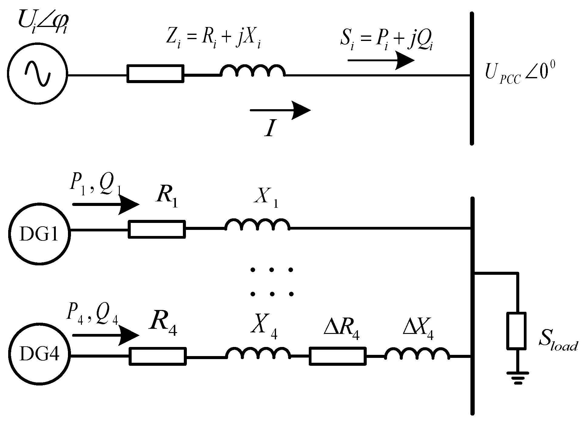
Within the low-voltage microgrid scenario comprising four heterogeneous DGs investigated in this work, the primary objective is to ensure that the dynamically varying total system load is shared among DG units strictly proportional to their rated capacity ratio of $S_{n1}:S_{n2}:S_{n3}:S_{n4}=1:1:2:2$, the equivalent circuit of which is illustrated in Figure 6. Nevertheless, the inevitable line impedance heterogeneity connecting individual units to the PCC deteriorates reactive power sharing precision, creating a risk of unit overloading. Furthermore, these impedance discrepancies precipitate circulating currents by inducing terminal voltage disparities among the parallel inverters.

Consider the $i$-th VSG characterized by an output terminal voltage phasor ${\dot{U}}_i=U_i\angle {\varphi }_i$, which is connected to the PCC via a line impedance $Z_i=R_i+j{X}_i$. Let the voltage phasor at the PCC be the reference phasor ${\dot{U}}_{pcc}=U_{pcc}\angle 0^{\circ }$. The complex power $S_i=P_i+j{Q}_i$ injected by the VSG into the PCC is expressed as

$$S_i={\dot{U}}_{pcc}{\dot{I}}_i^{\ast }={\dot{U}}_{pcc}{\left({\displaystyle \frac{{\dot{U}}_i-{\dot{U}}_{pcc}}{Z_i}}\right)}^{\ast }$$

(17)

where $S_i$ denotes the complex power output of the $\mathrm{i}$-th VSG; $I_i^{\ast }$ is the conjugate of the output current phasor; ${\dot{U}}_{pcc}$ represents the PCC voltage phasor; ${\dot{U}}_i$ signifies the output voltage phasor of the $\mathrm{i}$-th VSG; and $Z_i$ is the line impedance.

Expanding Equation (17) in phasor form and separating the real and imaginary components yields the nonlinear expression for reactive power $Q_i$:

$$Q_i={\displaystyle \frac{U_i{U}_{pcc}sin{\varphi }_i}{R_i^2+X_i^2}}{R}_i-{\displaystyle \frac{U_i{U}_{pcc}cos{\varphi }_i-U_{pcc}^2}{R_i^2+X_i^2}}{X}_i$$

(18)

where ${\varphi }_i$ denotes the power angle. Since ${\varphi }_i$ remains sufficiently small within the typical operating range of the VSG, the linear approximations $\mathrm{c}\mathrm{o}\mathrm{s}{\varphi }_{\mathrm{i}}\approx 1$ and $\mathrm{s}\mathrm{i}\mathrm{n}{\varphi }_{\mathrm{i}}\approx {\varphi }_{\mathrm{i}}$ are justified. Furthermore, considering that the terminal voltage magnitude ${\mathrm{U}}_{\mathrm{i}}$ approximates the PCC voltage, Equation (18) can be simplified as

$$Q_i\approx {\displaystyle \frac{U_i^2}{R_i^2+X_i^2}}\left[-R_i{\varphi }_i+X_i{\displaystyle \frac{\left(U_i-U_{pcc}\right)}{U_i}}\right]$$

(19)

It is evident from Equation (18) that the reactive power $Q_i$ is strongly correlated not only with its primary control variable, the voltage difference $U_i-U_{pcc}$, but also with the power angle ${\varphi }_i$. This coupling relationship compromises the validity of traditional droop control strategies based on P-f and Q-V decoupling assumptions.

To effectively suppress circulating currents among parallel units, it is imperative that the output terminal voltage amplitudes ${\mathrm{U}}_{\mathrm{i}}$ of all VSGs are maintained as consistently as possible. According to Equation (4), the condition for equalizing all ${\mathrm{U}}_{\mathrm{i}}$ is:

$$n_{q,i}(Q_i-Q_{0,i})=n_{q,j}(Q_j-Q_{0,j})=\cdots =n_{q,N}(Q_N-Q_{0,N})$$

(20)

Under the objective of capacity-based allocation, $n_{q,i}$ is typically inversely proportional to the rated reactive capacity $Q_{n,i}$, satisfying $n_{q,i}{Q}_{n,i}=K$. Consequently, the actual output reactive power $Q_i$ is required to be distributed strictly in proportion to capacity. However, since the value of $Q_i$ is co-determined by $U_i$, ${\varphi }_i$ and while also being significantly influenced by the line parameters $R_i$ and $X_i$, precise sharing cannot be achieved solely by voltage equalization.

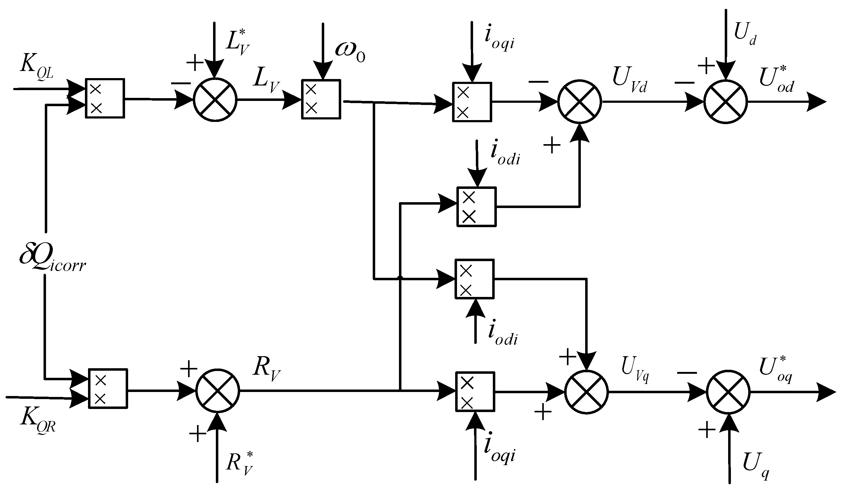
To address this challenge, an IAVI strategy is designed within the secondary cooperative control framework. As illustrated in Figure 7, the core philosophy is to generate a correction signal $\delta Q_{\mathit{corr}}$ via the secondary controller based on the reactive power sharing error, which is then utilized to dynamically modulate the virtual impedance value.

The normalized reactive power sharing error ${ϵ}_{q,i}$ is estimated via the consistency algorithm:

$${ϵ}_{q,i}={\sum }_{j\in N_i}{a}_{ij}\left(K_{q,i}{Q}_i-K_{q,j}{Q}_j\right)$$

(21)

Subsequently, the correction signal $\delta Q_{\mathit{conv},i}$ is generated through a PI controller:

$$\delta Q_{icorr,i}=K_{PQ,sec}\left(-c_q{ϵ}_{q,i}\right)+K_{IQ,sec}\int \left(-c_q{ϵ}_{q,i}\right)dt$$

(22)

where $c_q$ is the reactive power control gain of the consistency term; and $K_{PQ,sec},K_{IQ,sec}$ denote the proportional and integral coefficients of the reactive power PI controller, respectively. This correction signal is applied to adaptively adjust the virtual impedance:

$$\left\{\begin{array}{c}{R}_{v,i}=R_v^{\ast }+K_{QR}\cdot \delta Q_{\mathit{icorr},i}\\ L_{v,i}=L_v^{\ast }-K_{QL}\cdot \delta Q_{\mathit{icorr},i}\end{array}\right.$$

(23)

where $R_{v,i}$,$L_{v,i}$ denote the adaptive virtual resistance and inductance of the $\mathrm{i}$-th DG; $R_v^{\ast },{\hspace{0.33em}L}_v^{\ast }$ are the nominal setpoints; and $K_{QR},K_{QL}$ represent the adaptive regulation gains.

By utilizing the adaptive virtual impedance parameters derived from Equation (4) in conjunction with the inverter output current components in the dq frame, the virtual voltage drops $U_{v,d}$ and $U_{v,q}$ are formulated as:

$$\left\{\begin{array}{c}{U}_{vd,i}=R_{v,i}{i}_{odi}-{\omega }_0{L}_{v,i}{i}_{oqi}\\ U_{vq,i}=R_{v,i}{i}_{oqi}+{\omega }_0{L}_{v,i}{i}_{odi}\end{array}\right.$$

(24)

This voltage drop is directly subtracted from the primary voltage reference, achieving precise indirect regulation of reactive power.

To restore the system voltage to the nominal value, a voltage compensation signal $\Delta {\mathrm{U}}_{\mathrm{i}}$ is generated based on the consistency algorithm:

$$\left\{\begin{array}{c}\begin{array}{c}{\dot{U}}_{c,i}=-c_v{\sum }_{j\in N_i}{a}_{ij}\left(U_{o,i}-U_{o,j}\right)\\ e_{v,i}=U_0-\left(U_{o,i}+U_{c,i}\right)\end{array}\\ \Delta U_i=\int e_{v,i}dt\end{array}\right.$$

(25)

Substituting Equation (24) into the primary Q-V droop loop results in the zero-error regulation of the final voltage:

$$U=U_0-K_{q,i}\left(Q_i-Q_{0,i}\left(t\right)\right)+\Delta U_i$$

(26)

4. Adaptive Particle Swarm Optimization Algorithm

In islanded microgrids incorporating secondary cooperative control, the dynamic response characteristics of the underlying voltage and current dual-loop controllers directly dictate the system’s dynamic performance during load fluctuations and secondary regulation processes. Given the strong coupling and nonlinear features of multi-machine parallel microgrid systems, conventional empirical tuning methods struggle to strike an optimal balance between system rapidity and stability under complex disturbances. To this end, this paper transforms the optimization of VSG dual-loop parameters into a global cooperative optimization process under multidimensional constraints. In this model, the optimization variables are defined as a four-dimensional position vector $x=\left[K_{pv},K_{iv},K_{pc},K_{ic}\right]$, comprising the proportional and integral coefficients of the voltage and current loops. To ensure the symmetry of the equivalent output impedance and fundamentally mitigate high-frequency reactive circulating currents caused by parameter mismatch, the algorithm constrains all DG units within the microgrid to adopt identical controller parameter configurations, with the search space strictly confined within the predefined stability region of the control system.

Conventional steady-state error metrics are insufficient for capturing the intensity of transient oscillations and the damping characteristics during disturbances. Consequently, this paper establishes a comprehensive objective function $J$ based on the ITAE criterion to quantitatively assess the cumulative deviations of system voltage and frequency throughout the complete dynamic evolution process:

$$J={\int }_{T_0}^{T_1}t\cdot \left(w_v{\sum }_{i=1}^N\left|U_0-U_i\left(t\right)\right|+w_f{\sum }_{i=1}^N\left|f_0-f_i\left(t\right)\right|\right)dt$$

(27)

where $T_0$ is the evaluation start time (set to 0.3 s) to assess the dynamic recovery capability after the control strategy intervention; $T_1$ is the simulation end time (set to 1.5 s); $N$ denotes the number of DGs; $U_i\left(t\right)$ and $f_i\left(t\right)$ represent the real-time output voltage amplitude and frequency of the $i$-th DG, respectively; $w_v$ and $w_f$ are weighting coefficients used to balance the optimization priorities of voltage and frequency. Since the numerical value of frequency deviation (typically <0.2 Hz) is far smaller than that of voltage deviation, to balance the dimensional disparity, it is typically set that $w_f>w_v$. By introducing the time multiplier $\mathrm{t}$, the objective function imposes progressively severe mathematical penalties on sustained oscillations during the later stages of the transient process. This mechanism effectively drives the optimization algorithm to identify a global optimal parameter set that simultaneously ensures rapid response, minimal overshoot and steady-state error.

While SPSO offers efficient global search capabilities via swarm intelligence, it is inherently susceptible to premature convergence and entrapment in local optima, particularly when navigating high-dimensional multimodal objective functions. The inertia weight $\omega$ serves as a critical parameter governing the trade-off between the algorithm’s global exploration and local exploitation. Consequently, to mitigate these limitations and enhance convergence precision, a nonlinear dynamic adaptive inertia weight mechanism is introduced herein.

In the proposed APSO framework, the velocity vector $v_{id}^{k+1}$ and position vector $x_{id}^{k+1}$ of the $i$-th particle at the $k$-th iteration are updated according to the following evolution equations:

$$\left\{\begin{array}{c}{v}_{id}^{k+1}=\omega \left(k\right)v_{id}^k+c_1{r}_1\left(P_{\mathit{best},\mathit{id}}^k-x_{id}^k\right)+c_2{r}_2\left(G_{\mathit{best},d}^k-x_{id}^k\right)\\ x_{id}^{k+1}=x_{id}^k+v_{id}^{k+1}\end{array}\right.$$

(28)

where $\mathrm{d}$ denotes the dimensionality of the search space (set to 4); $\omega \left(k\right)$ epresents the time-varying inertia weight; $c_1,c_2$ are the cognitive and social acceleration coefficients, respectively (both set to 2.0), which govern the particle’s tendency to move towards its personal historical best $\left(P_{\mathit{best}}\right)$ and the global swarm best $\left(G_{\mathit{best}}\right)$; and $r_1,r_2$ are random variables uniformly distributed in the range $\left[0,1\right]$, introduced to enhance the stochasticity of the search process.

To strike a balance between extensive global exploration in the initial phase and refined local exploitation in the final phase, a nonlinear dynamic decreasing strategy for the inertia weight $\omega \left(k\right)$ is employed:

$$\omega \left(k\right)={\omega }_{max}-\left({\omega }_{max}-{\omega }_{min}\right)\times {\left({\displaystyle \frac{K}{K_{max}}}\right)}^2$$

(29)

where ${\omega }_{max}$ and ${\omega }_{min}$ define the upper and lower bounds of the inertia weight, set to 0.9 and 0.4, respectively; $K$ and $K_{max}$ denote the current and maximum iteration counts. This nonlinear profile ensures high inertia initially to facilitate escape from local extrema, while progressively reducing inertia to accelerate convergence speed near the global optimum. The specific parameter configuration of the APSO algorithm is tabulated in

Table 1. Parameter settings of the APSO algorithm.

Parameter	Value/Range
Population Size ($N$)	20
Max Iterations ($K_{max}$)	30
Learning Factors ($c_1,c_2$)	2.0, 2.0
Inertia Weight (${\omega }_{max},{\omega }_{min}$)	0.9, 0.4
Voltage Loop Proportional Coeff ($K_{pv}$)	$[0.1,50.0]$
Voltage Loop Integral Coeff ($K_{iv}$)	$[10,800]$
Current Loop Proportional Coeff ($K_{pc}$)	$[0.1,50.0]$
Current Loop Integral Coeff ($K_{ic}$)	$[10,800]$
Voltage Error Weight ($w_v$)	1.0
Frequency Error Weight ($w_f$)	5.0

.

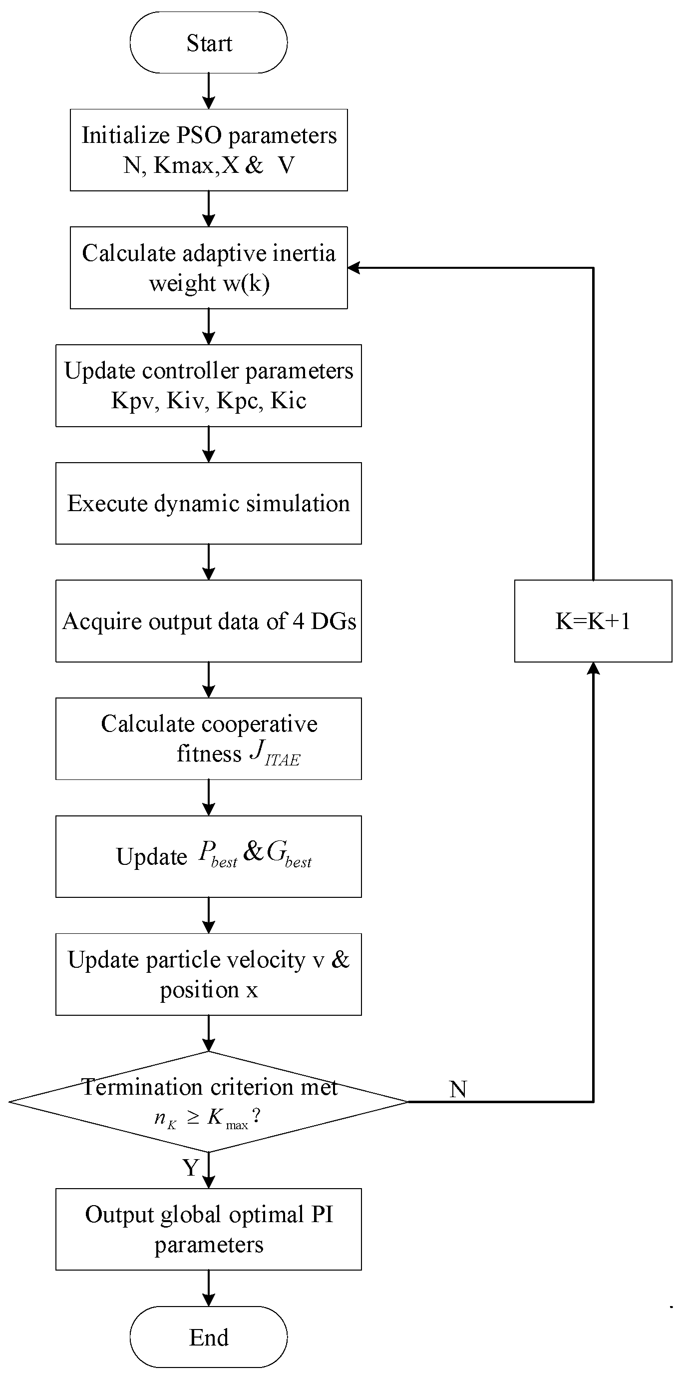
Building upon the aforementioned mathematical formulation and evaluation criteria, the APSO algorithm is utilized to perform the cooperative optimization task. Within each iterative cycle, the algorithm initiates by injecting the candidate PI parameter configurations, represented by the current swarm of particles, into the Simulink-based physical model. Subsequently, a time-domain simulation is executed, subjected to a step-load disturbance. Following the simulation, the data acquisition module extracts the full time-domain voltage and frequency response trajectories across the evaluation window, which are then substituted into J to determine the corresponding fitness value. At the core layer of the algorithm, a logical judgment unit facilitates a real-time comparison between the current fitness value and $P_{\mathit{best}}$ and $G_{\mathit{best}}$. Should the predefined update criteria be satisfied, the particle parameters are refined via evolutionary operators. This iterative process continues until the maximum iteration count is reached. The detailed execution procedure and the integrated joint-simulation logic are illustrated in Figure 8.

5. Simulation Results

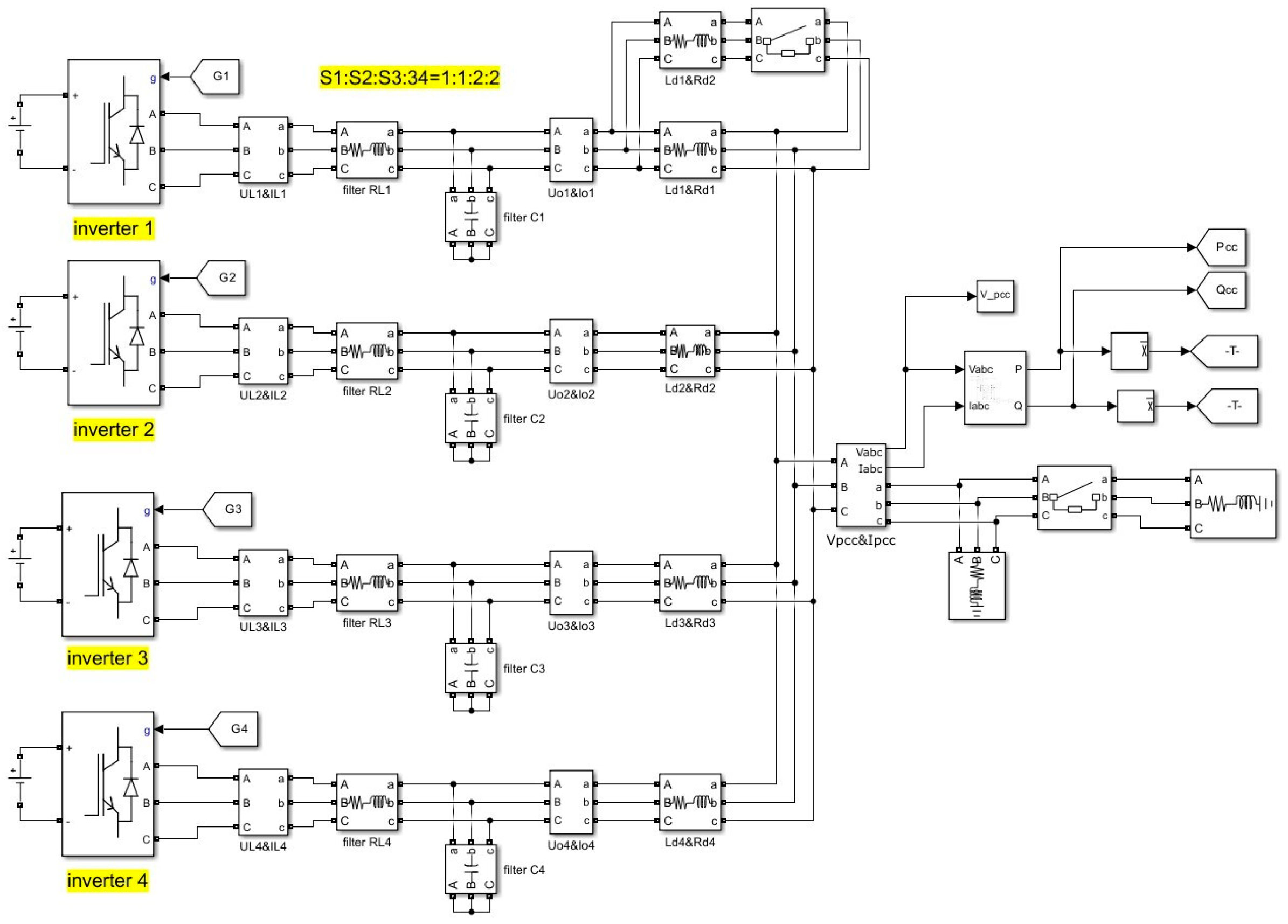
To rigorously validate the efficacy and superiority of the hierarchical cooperative control strategy based on load feedforward and particle swarm optimization proposed herein, a comprehensive islanded microgrid simulation platform comprising four heterogeneous DG units was constructed within the MATLAB/Simulink 2024b environment. In this model, four independent VSG inverter units are interfaced in parallel with the PCC via resistive-inductive line impedances possessing distinct parameters, denoted as $Ld1$ & $Rd1$ through $Ld4$ & $Rd4$. Each VSG unit incorporates an ideal DC voltage source, a three-phase inverter bridge, an LC filter, and its specific primary controller. The aggregate system load comprises a local load and a switchable disturbance load, both coupled to the PCC. To faithfully emulate the inherent heterogeneity of the system, the rated capacity ratio of the four VSG inverters is configured as $S_{n1}:S_{n2}:S_{n3}:S_{n4}=1:1:2:2$, with the detailed topological structure depicted in Figure 9.

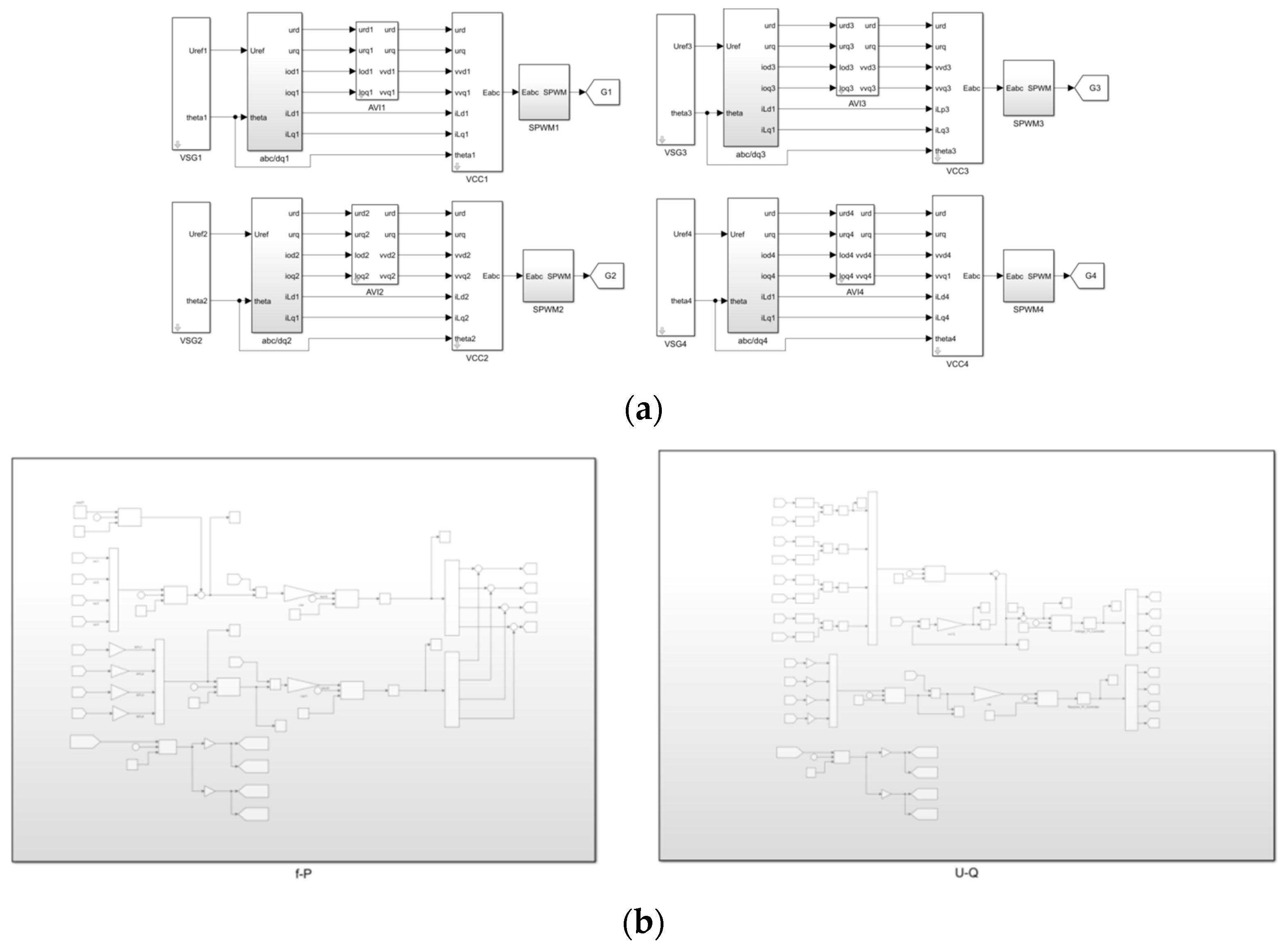
The overarching architecture of the hierarchical cooperative control system is schematized in Figure 10. Figure 10a delineates the primary control layer deployed locally on the four DGs, where each controller receives frequency and voltage compensation signals from the secondary layer and synthesizes the reference voltage vector U and phase $\theta$ based on the droop mechanism. These references undergo abc/dq coordinate transformation to yield d-q frame components, which, in coordination with the outputs from the IAVI module and inner-loop decoupling terms, constitute the input vector for the voltage and current dual-loop controller. The voltage and current control module subsequently outputs the three-phase modulation reference ${\mathrm{E}}_{\mathrm{a}\mathrm{b}\mathrm{c}}$, which generates the driving pulses via the SPWM module to regulate the inverter. Figure 10b presents the global secondary cooperative control layer; the left panel displays the P-f cooperative controller, while the right panel shows the Q-V cooperative controller, employed to generate restoration compensation signals for frequency and voltage, respectively. Furthermore, the LODRF module utilizes real-time load data acquired at the PCC to proactively generate power sharing references for each DG.

The dynamic load profile of the system is programmed as follows: during the interval [0 s, 0.5 s], the system sustains a base load of 36 kW active power and r reactive power; at t = 0.5 s, the load serves a step increment of 100%, reaching an aggregate demand of 72 kW + 48 kVar; at t = 1.0 s, load shedding occurs where the load is halved, instantaneously returning the system to its initial state. The detailed electrical and control parameters employed in the simulation are tabulated in

Table 2. System simulation parameters.

Parameter	DG1	DG2	DG3	DG4
DC Bus Voltage $U_{\mathit{dc}}$ (V)	800
Rated Phase Voltage $U_o$ (V)	311
Rated Frequency $f_o$ (Hz)	50
Filter Inductance $L_f$ (mH)	2.0
Filter Resistance $R_f$ (Ω)	0.01
Filter Capacitance $C_f$ (μF)	50
Line Resistance (Ω)	0.64	0.8	0.23	0.37
Line Inductance (μH)	5.0	3.0	4.0	6.0
Virtual Resistance $R_v^{\ast }$ (Ω)	0.080	0.001	0.078	0.090
Virtual Inductance $L_v^{\ast }$ (mH)	3.90	3.96	1.98	8.00
Active Droop Coeff. $K_p$ (rad/s/W)	3.0 × 10−5	3.0 × 10−5	1.5 × 10−5	1.5 × 10−5
Reactive Droop Coeff. $K_q$ (V/Var)	2.0 × 10−5	2.0 × 10−5	1.0 × 10−5	1.0 × 10−5
Virtual Inertia J	0.2	0.2	0.4	0.4
Virtual Damping D	80	80	160	160
Freq. Recovery Gain $c_{\omega }$	100
Volt. Recovery Gain $c_v$	100
Active Sharing Gain $c_p$	10
Reactive Sharing Gain $c_q$	10
SPSO-optimized Voltage Loop $K_{pv},K_{iv}$	3.1726, 163.4783
SPSO-optimized Current Loop $K_{pc},K_{ic}$	8.8336, 230.7629
APSO-optimized Voltage Loop $K_{pv},K_{iv}$	2.5806, 56.7831
APSO-optimized Current Loop $K_{pc},K_{ic}$	20.4192, 156.4239

.

5.1. Conventional Primary Control

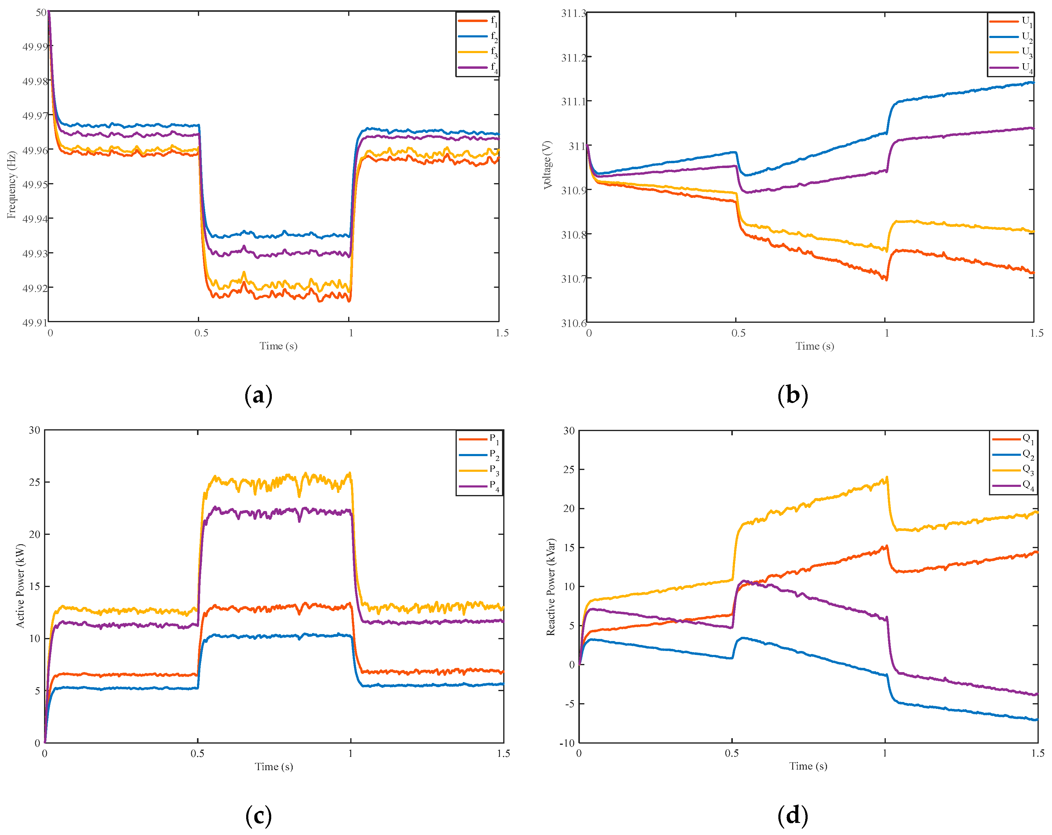
To elucidate the inherent limitations of conventional control strategies, this section first evaluates the system’s dynamic performance operating solely under traditional droop control without the integration of the IAVI module. The objective is to rigorously verify the direct detrimental impact of line impedance mismatches and P-Q coupling on stable system operation. The simulation results are presented in Figure 11.

As detailed in Figure 11a, governed by the inherent steady-state error characteristic of droop control, the system frequency consistently deviates below the nominal $50 \mathrm{H}\mathrm{z}$ throughout the $[0, 0.5 \mathrm{s}]$ interval, experiencing an exacerbated dip following the load step at $0.5 \mathrm{s}$. Moreover, the frequency trajectories of the individual DGs fail to synchronize, exhibiting sustained, asynchronous low-frequency oscillations. In Figure 11c, the DGs fail to share the active power load in proportion to their rated capacities, a phenomenon accompanied by significant power fluctuations.

Attributable to severe line impedance mismatches, Figure 11b exposes pronounced disparities in the output terminal voltages of the DGs. This voltage imbalance directly compromises the reactive power distribution mechanism. Consequently, as depicted in Figure 11d, the reactive power outputs diverge significantly from the theoretical $1:1:2:2$ sharing ratio, thereby exciting high-frequency circulating currents among the inverters, which further aggravates system instability.

5.2. Primary Control Based on IAVI and Control Parameter Optimization

Addressing the limitations of conventional primary control, this section integrates the IAVI module into the primary control architecture. Simultaneously, acknowledging that the dynamic performance is heavily contingent upon the tuning of the underlying voltage and current dual-loop PI parameters, this study compares the efficacy of different optimization algorithms. The parameters are calibrated using SPSO with fixed inertia weight and the proposed APSO, respectively, where the specific optimized parameters are detailed in Table 2. The subsequent figures illustrate the dynamic profiles of system frequency, voltage, active power and reactive power following the introduction of IAVI under these two distinct optimization strategies.

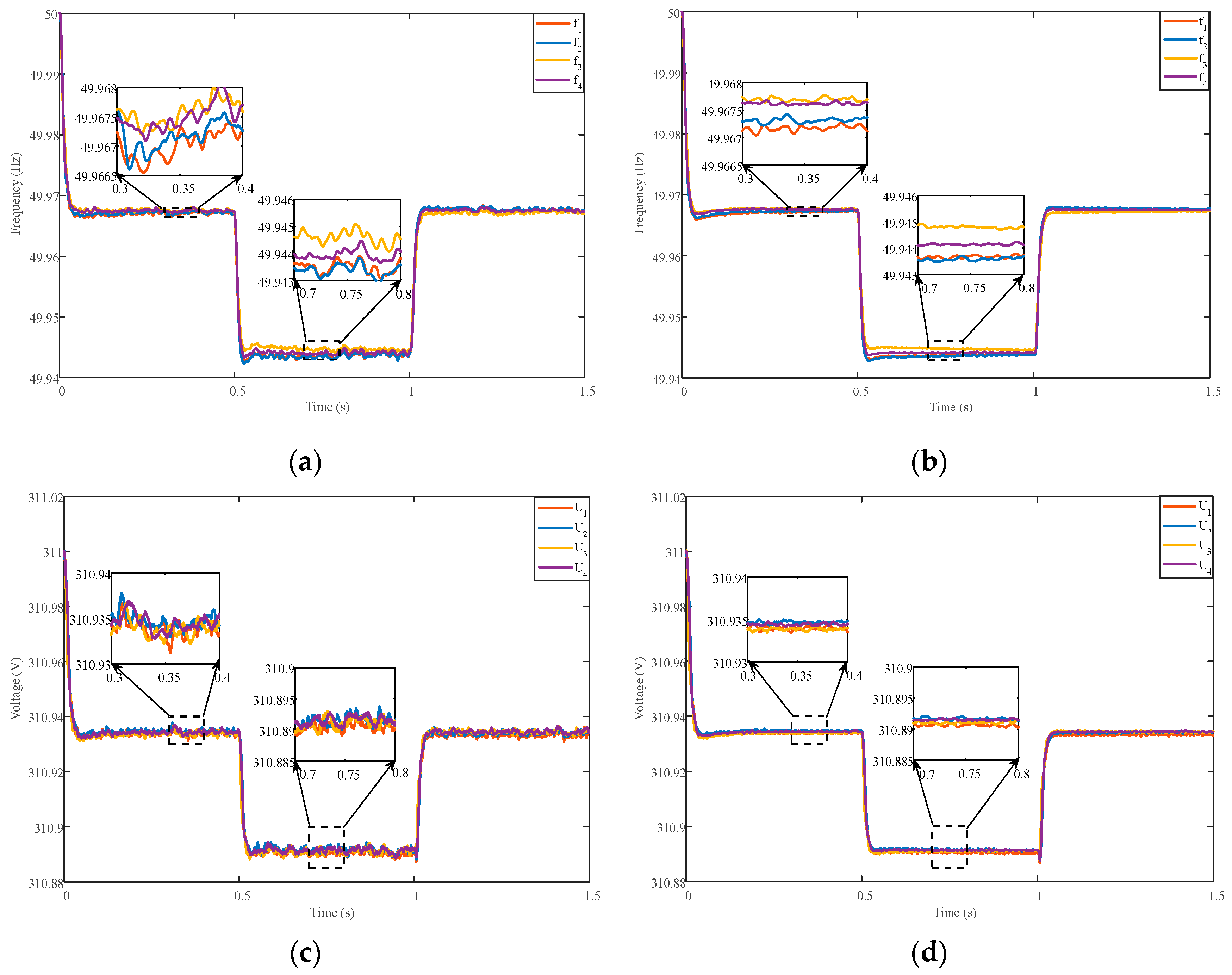
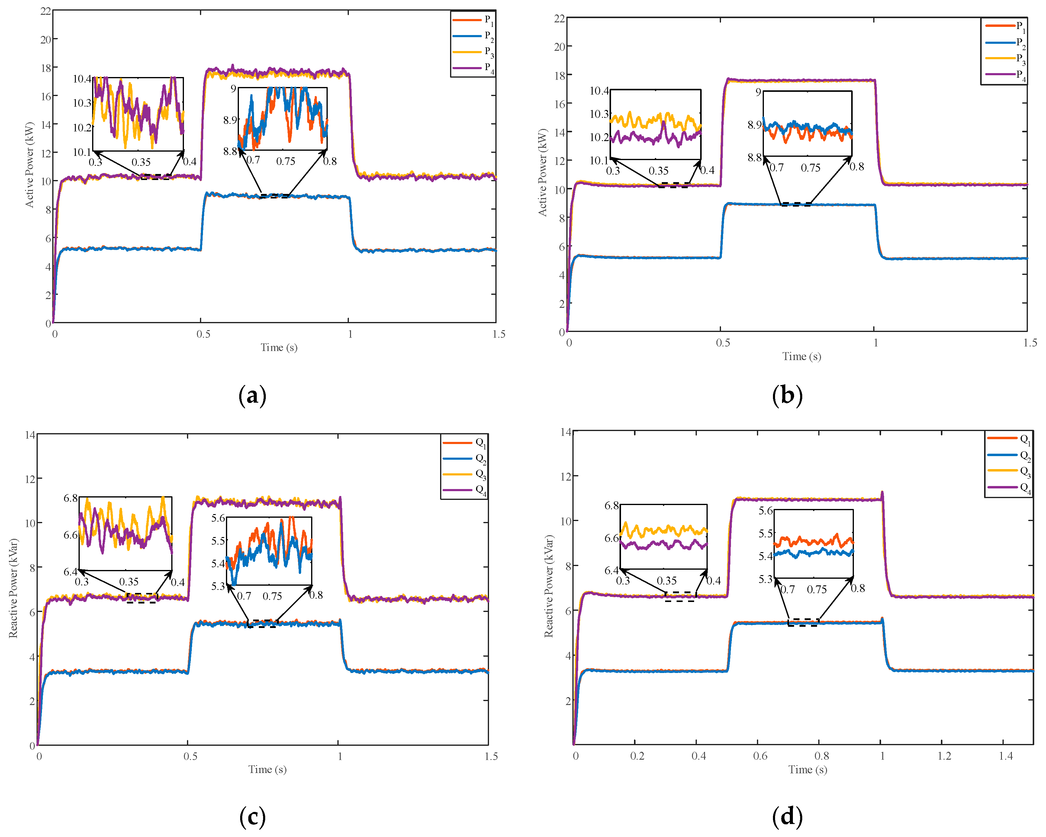
A comparative analysis with Figure 11 reveals that, as shown in Figure 12, the frequency and voltage curves of all DGs achieve rapid convergence post-optimization, thereby validating the efficacy of IAVI in decoupling and stabilizing the system. Furthermore, by contrasting the SPSO results depicted in Figure 12a,c with the APSO results shown in Figure 12b,d, it is evident that the trajectories optimized by APSO are significantly smoother with minimized fluctuation ranges. This indicates that the system exhibits superior damping characteristics and robustness following APSO. However, constrained by the inherent regulatory nature of primary control, the frequency of the four DGs hovers around $49.967 \mathrm{Hz}$ during $[0, 0.5 \mathrm{s}]$, and the output voltage settles near $310.935 \mathrm{V}$, with further deviations occurring after the load doubles in the $[0.5, 1 \mathrm{s}]$ interval.

As illustrated in Figure 13, the power outputs for all DGs accurately adhere to the 1:1:2:2 rated capacity ratio under both SPSO and APSO schemes upon the integration of the IAVI mechanism. However, the proposed APSO strategy demonstrates superior execution performance. During the [0, 0.5 s] interval, high-frequency oscillations of approximately 0.3 kW and 0.2 kVar are observed in $P_{\mathrm{3,4}}$ and $Q_{\mathrm{3,4}}$ under SPSO. In contrast, the steady-state fluctuations of active and reactive power are effectively suppressed within 0.1 kW and 0.1 kVar by the APSO strategy during the same period. Similarly, during the load step interval of [0.5, 1 s], $P_{\mathrm{1,2}}$ and $Q_{\mathrm{1,2}}$ are stabilized at approximately 8.9 kW and 5.45 kVar by the APSO algorithm. Conversely, the power outputs under SPSO exhibit significant ripples, fluctuating between 8.8 and 9.1 kW for active power and between 5.3 and 5.6 kVar for reactive power. The numerical superiority of APSO regarding waveform smoothness and oscillation suppression validates its enhanced efficiency for searching optimal solutions within complex and high-dimensional parameter spaces.

In practical microgrid operation, line impedance frequently undergoes dynamic variations due to network reconfiguration, feeder switching, or environmental factors. To evaluate the adaptive capability of the strategy proposed in this paper under network parameter fluctuations, a line impedance perturbation experiment was conducted.

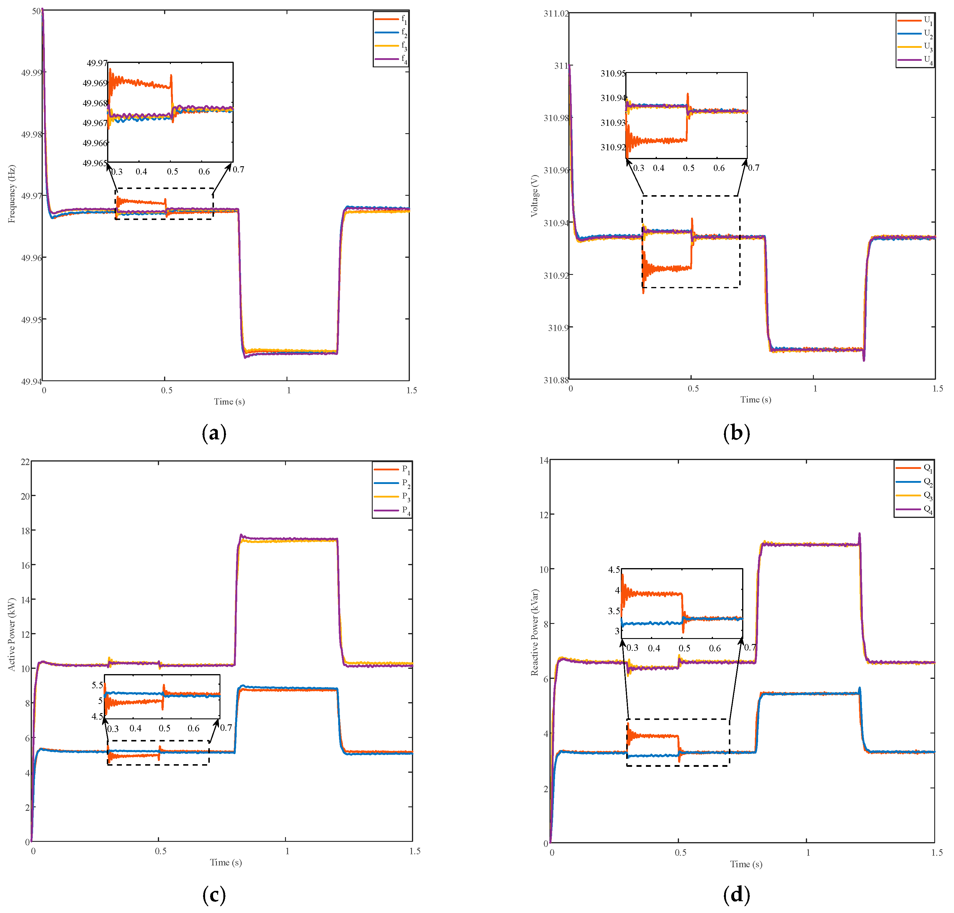
The system initially operates at rated conditions. At t = 0.3 s, the line impedance of DG₁ was subjected to a sudden 50% reduction through parallel equivalent branches, the detailed simulation design of which is depicted in Figure 9. As illustrated in Figure 14, since all units initially maintained fixed virtual impedance parameters, the frequency ${\mathrm{f}}_1$ manifested a deviation to 49.969 Hz, and the voltage ${\mathrm{U}}_1$ dropped to 310.92 V. Simultaneously, the active and reactive power outputs of DG1 deviated from the theoretical setpoints by 0.25 kW and 0.58 kVar, respectively. Following the activation of the adaptive virtual impedance adjustment at t = 0.5 s, the virtual resistance $R_{v1}^{\ast }$ of DG1 was reconfigured to 0.24 Ω, and the virtual inductance was updated to 3.87 mH. Consequently, all electrical variables rapidly converged to their theoretical steady-state values. The system maintained stability during the load doubling at [0.8, 1.2 s] and load shedding at [1.2, 1.5 s], accurately tracking the theoretical power sharing trajectories. These results demonstrate that the proposed strategy can ensure precise power allocation and maintain operational robustness via parameter reconfiguration even when the physical network structure undergoes severe perturbations.

5.3. Hierarchical Cooperative Control

To remediate the inherent limitations of primary control regarding steady-state deviations and imprecise power sharing, and to rigorously validate the superiority of the proposed APSO algorithm in terms of convergence efficacy and optimization quality, a comparative analysis between APSO and SPSO was conducted within the hierarchical cooperative control framework. The specific algorithmic parameters are detailed in Table 1. In the simulation sequence, the complete secondary control layer is activated at $t=0.3 \mathrm{s}$. Subsequently, the system is subjected to a load doubling at $t=0.5 \mathrm{s}$, reaching a peak aggregate load of $72 \mathrm{kW}+48 \mathrm{kVar}$, followed by a load shedding event at $t=1.0 \mathrm{s}$ where the load returns to its initial state of $36 \mathrm{kW}+24 \mathrm{kVar}$. The simulation duration is fixed at $0.5 \mathrm{s}$, with the optimization objective defined as the weighted ITAE for frequency and voltage over the interval $[0.5, 1 \mathrm{s}]$. 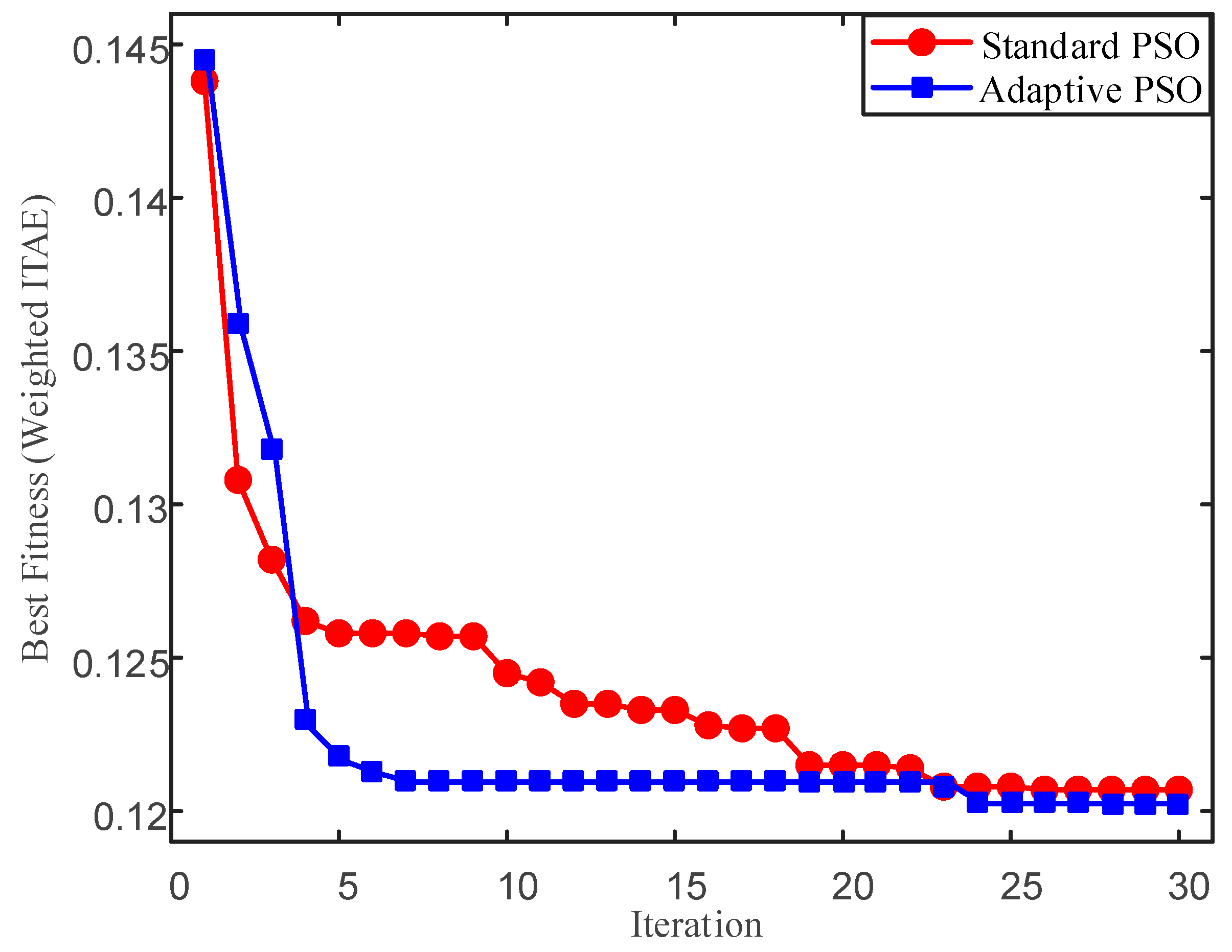The convergence trajectories of the iterative process are illustrated in Figure 15.

As depicted in Figure 15, while both algorithms eventually converge to a low fitness value, the APSO algorithm exhibits significantly superior convergence characteristics compared to SPSO. Although SPSO demonstrates a rapid initial descent, it succumbs to premature convergence after the 10th iteration, characterized by stagnation in fitness value reduction. In stark contrast, the APSO algorithm converges to a superior fitness value (ITAE = 0.122936) within merely five iterations and maintains stability thereafter. This evidence underscores APSO’s enhanced capability to balance global exploration and local exploitation throughout the iterative process, thereby achieving swifter and deeper convergence.

The post-optimization performance indices are tabulated in

Table 3. Comparison of system performance indices after SPSO and APSO.

Optimization Algorithm	Overshoot (%)		RMSE		Max Freq. Dev. (Hz)	Max Volt. Dev. (V)	Avg. Active Power Sharing Error (%)	Avg. Reactive Power Sharing Error (%)
	Freq.	Volt.	Freq.	Volt.
SPSO	0.0064	0.0031	0.0004	0.0013	0.0032	0.022	0.8698	0.9747
APSO	0.0063	0.0030	0.0004	0.0012	0.0031	0.014	0.7030	0.8150

. While marginal differences are observed in overshoot and RMSE, the maximum frequency and voltage deviations optimized by APSO are restricted to 0.0031 Hz and 0.014 V, representing substantial reductions of 3.1% and 36.4%, respectively, relative to the SPSO baseline. Regarding steady-state precision, the average active and reactive power sharing errors under APSO are both maintained below 0.9%, corresponding to improvements of 19.2% and 16.4% over SPSO. These metrics unequivocally demonstrate the superiority of the proposed APSO algorithm in minimizing steady-state errors and enhancing allocation accuracy.

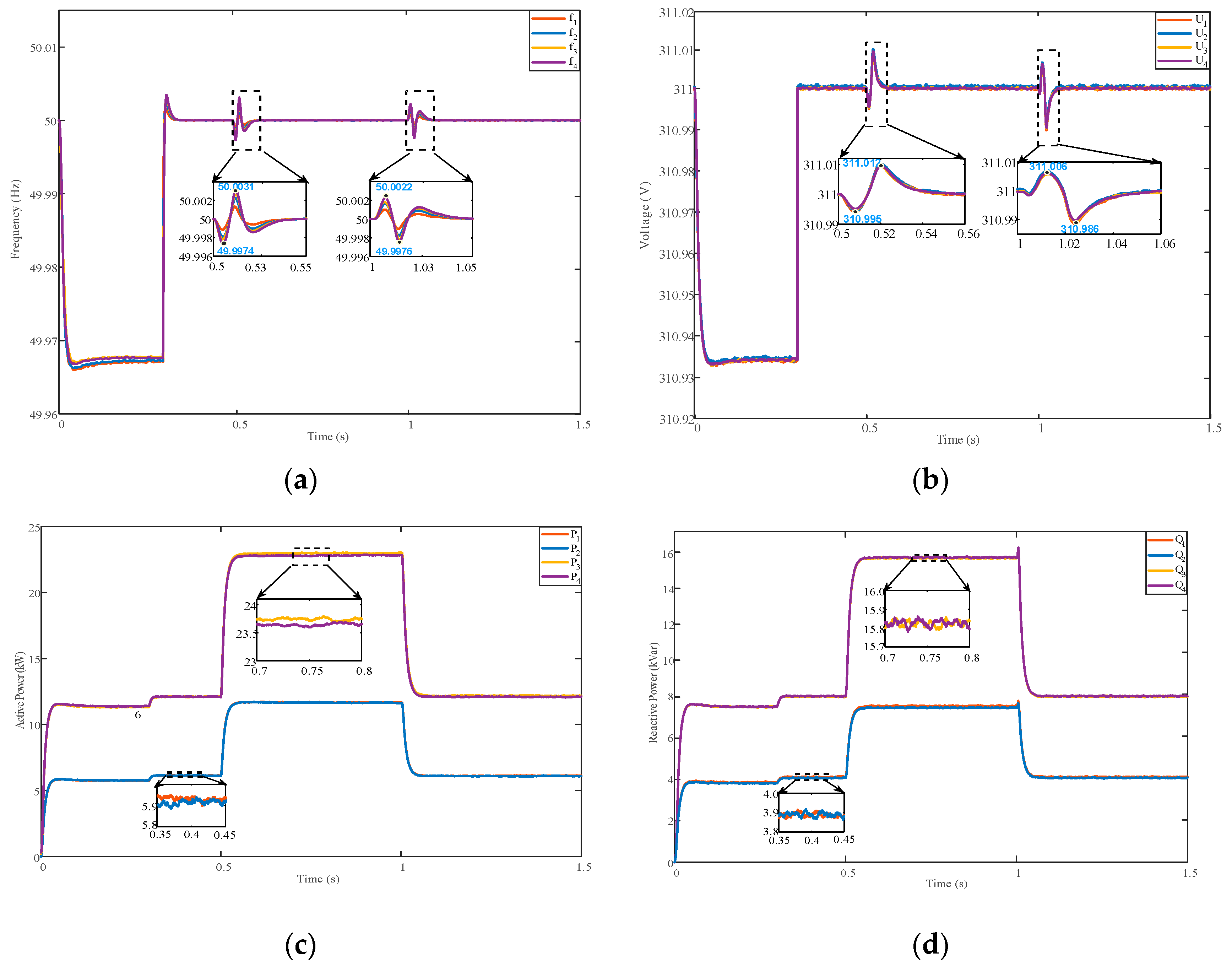
The system dynamic response under the optimal parameter configuration derived from APSO is illustrated in Figure 16a,b display the frequency and terminal voltage profiles, while Figure 16c,d present the active and reactive power output trajectories.

As observed in Figure 16a,b, following the engagement of secondary control at t = 0.3 s, the steady-state deviations in frequency and voltage are rapidly eliminated, with values being precisely restored to 50 Hz and 311 V. Even under severe load step disturbances at t = 0.5 s and t = 1.0 s, the system retains robust recovery capabilities. Notably, the transient frequency and voltage deviations are capped at 0.0031 Hz and 0.014 V, accompanied by a swift settling time and negligible oscillation.

Regarding power allocation, as shown in Figure 16c,d, the output power of each DG at t = 0.3 s is calibrated strictly to its theoretical setpoint, maintaining the requisite 1:1:2:2 ratio. Specifically, during the interval [0.3 s, 0.5 s], $P_{\mathrm{1,2}}\approx 6 \mathrm{k}\mathrm{W}$ and $Q_{\mathrm{1,2}}\approx 4 \mathrm{k}\mathrm{V}\mathrm{a}\mathrm{r}$; during [0.5 s, 1.0 s], $P_{\mathrm{3,4}}\approx 24 \mathrm{k}\mathrm{W}$ and $Q_{\mathrm{3,4}}\approx 16 \mathrm{k}\mathrm{V}\mathrm{a}\mathrm{r}$, with steady-state errors consistently suppressed below 0.9%. These results effectively corroborate the precision of the proposed strategy in power sharing.

Furthermore, to verify the dynamic enhancement provided by the LODRF strategy, a comparative analysis was performed under identical conditions. The simulation results prior to the inclusion of the LODRF module are presented in Figure 17.

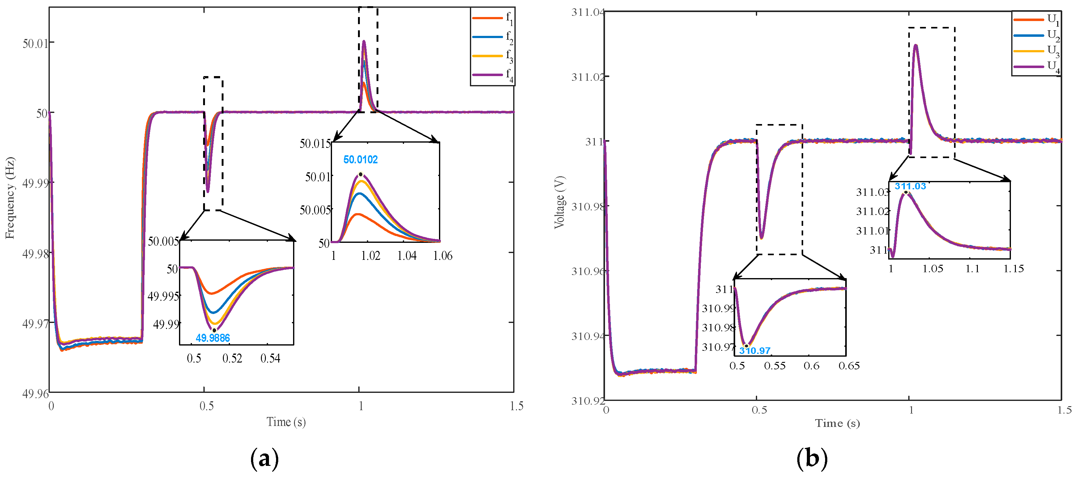
Analysis of Figure 17 reveals that without LODRF, the maximum frequency and voltage deviations under load disturbance at t = 0.5 s reach 0.0144 Hz and 0.03 V. Comparing these benchmarks with the results in Figure 16a,b, it is evident that the proposed LODRF strategy attenuates the maximum dynamic deviations of frequency and voltage by 78.5% and 53.3%, respectively. Moreover, the effective recovery times are shortened by approximately 0.01 s and 0.09 s. This serves as compelling evidence of the improvements LODRF confers upon transient stability and rapid recovery capability.

6. Conclusions and Outlook

6.1. Conclusions

Addressing the challenges of precise power sharing imbalances and dynamic instability in frequency and voltage triggered by line impedance heterogeneity and load fluctuations in islanded microgrids, this paper proposes and validates a hierarchical cooperative control strategy fusing LODRF and APSO. Through detailed simulation analysis of a four-unit heterogeneous parallel microgrid system under multiple disturbance scenarios, the following conclusions are drawn:

• In scenarios characterized by severe line impedance mismatches, the introduction of the consistency-based IAVI technology effectively compensates for line voltage drop discrepancies, successfully eliminating system circulating currents and achieving the stable convergence of frequency and voltage as well as proportional power sharing.
• With the incorporation of the LODRF mechanism, the system effectively overcomes the response hysteresis inherent in traditional error feedback regulation. Under identical load step disturbances, compared with strategies lacking the feedforward policy, the proposed method significantly reduces the maximum dynamic deviations of system frequency and voltage, while shortening their effective recovery times.
• The comprehensive hierarchical cooperative strategy proposed herein realizes rapid recovery of frequency and voltage under load disturbance conditions, along with capacity-based power allocation. Following the optimization of controller parameters via the APSO algorithm, the system operational trajectories become notably smoother, exhibiting superior steady-state precision and dynamic robustness.

6.2. Outlook

Although the consistency-based hierarchical cooperative control strategy integrating LODRF and APSO proposed in this paper demonstrates significant performance enhancements in the simulation environment, several research directions warrant further in-depth investigation:

• This study primarily focuses on a four-unit inverter system. As the number of inverters increases, the system may confront challenges such as more complex inter-machine oscillation modes, cumulative communication delays, and coordination difficulties. Future work could explore extending the proposed hierarchical strategy to large-scale microgrids containing a greater number and more diverse types of distributed energy resources, ensuring that the strategy maintains its superior performance in large-scale distributed networks.
• Although the APSO algorithm has effectively optimized system performance, the topological structures and operating conditions in practical microgrids may vary dynamically, rendering fixed parameters tuned offline difficult to maintain as optimal. Future research could be dedicated to developing computationally efficient online optimization algorithms to meet the requirements of real-time microgrid control.
• The current research conclusions are primarily based on MATLAB/Simulink numerical simulations. The performance of control algorithms on physical hardware is subject to multiple physical factors such as computational latency, sensor noise, and non-ideal characteristics of power devices. Future efforts will involve establishing a hardware-in-the-loop experimental platform comprising real converters and controllers to further validate the effectiveness and engineering applicability of the proposed strategy.
• Future research could investigate the system performance under nonlinear and unbalanced loads. By introducing harmonic suppression and negative sequence regulation control, the robustness of the proposed hierarchical coordination strategy could be further evaluated in asymmetrical or distorted environments.