A Pre-Disaster Deployment and Post-Disaster Restoration Method Considering Coupled Failures of Power Distribution and Communication Networks

Abstract

Extreme natural disasters may simultaneously disrupt power distribution infrastructures and their supporting communication systems, significantly degrading post-disaster recovery performance. To enhance coordinated restoration under such coupled failure conditions, this study proposes a unified optimization framework for pre-disaster deployment and post-disaster repair and service restoration in interdependent distribution–communication networks. First, an interdependency model is developed to characterize the physical and operational couplings between the distribution and communication networks. The impacts of communication outages on remotely controlled switches and repair crew dispatching are quantitatively analyzed, revealing how communication failures influence the restoration process. Based on this interdependency representation, a coordinated optimization model is established to jointly determine repair crew routing, mobile power allocation, and critical load restoration sequencing. The objective is to minimize cumulative outage losses over the recovery horizon, thereby achieving coordinated allocation and routing of multiple types of emergency repair resources. Furthermore, by jointly considering pre-disaster deployment planning and post-disaster restoration strategies, a two-stage emergency recovery framework is designed to integrate pre-event preparedness with post-event response for distribution networks. Case studies on a modified IEEE 33-bus cyber–physical distribution system demonstrate that the proposed coordinated restoration strategy restores approximately 50% of critical loads within the first 3 h, which is of direct significance for maintaining essential services such as hospitals and emergency shelters during the acute phase of a disaster. The proposed approach reduces the total load loss by 49.5% and shortens the restoration time by 120 min. In terms of pre-disaster deployment, the proposed strategy reduces average load shedding by 33.4% and 46.5% relative to the heuristic and random deployment strategies, respectively, demonstrating the effectiveness of proposed method for grid resilience enhancement.

1. Introduction

In recent years, extreme events triggered by global climate change have occurred with increasing frequency. Natural disasters such as typhoons, heavy rainfall, and flooding have intensified in both magnitude and occurrence, posing significant threats to the secure and stable operation of power systems [1]. In 2024, the super typhoon Yagi made landfall along the coast of Hainan Province, resulting in 139 outages of 10 kV distribution lines and an outage rate as high as 82.3%. The direct economic losses were estimated at 32.7 billion RMB [2]. Under such extreme weather conditions, power systems urgently require enhanced resilience to withstand major disasters and maintain operational stability. Power system resilience refers to the ability of the grid to minimize the impact of low-probability but high-consequence events, ensure continuous supply to critical loads, and rapidly restore interrupted services [3,4]. In this context, pre-disaster deployment and post-disaster power restoration has become a central research focus.

Existing post-disaster restoration strategies primarily rely on local switching operations and distributed energy resources (DERs) to partition the distribution network into multiple independently operated microgrids, thereby maintaining the supply of critical local loads [5]. Although such strategies effectively support non-faulted areas, they also present limitations. Extreme disasters often cause extensive damage to distribution lines, preventing the system from promptly returning to its pre-disturbance operating state [6]. Furthermore, the limited capacity of local DERs constrains the effectiveness of islanded operation in satisfying overall load demand. Therefore, in addition to utilizing local resources, effective restoration requires coordinated dispatch of emergency repair resources, including repair crews and mobile power sources, to rapidly repair faulted lines and shorten system restoration time [7]. Such coordinated strategies contribute to faster recovery of normal operation and enhanced grid resilience. Reference [8] established a post-hurricane distribution network restoration model for allocating repair crew tasks; however, this approach focused solely on electrical topology and simplified crew dispatch into a binary assignment problem without fully modeling routing decisions. Reference [9] proposed coordinated supply restoration and fault repair strategies to accelerate distribution network recovery while maximizing load restoration. Reference [10] developed a mixed-integer linear programming model integrating post-disaster restoration and fault repair to minimize load loss during recovery. References [11,12] further proposed a coordinated optimization framework involving repair crews, mobile energy storage, and microgrids equipped with controllable power flow devices to accelerate critical load restoration. Nevertheless, most existing post-disaster restoration studies focus only on the distribution network and assume that the communication system remains fully functional throughout the restoration process. Under extreme disasters, however, communication facilities may also be damaged together with distribution lines, which directly impairs the operation of remotely controlled switches, weakens system observability, and delays restoration decision-making [13]. Since communication failures may prevent timely acquisition and transmission of fault information, ignoring the communication network may lead to an overly simplified representation of the actual restoration process.

A few recent studies have considered coupled failures of distribution and communication networks. For example, existing works have modeled the interdependence between the two networks and explored joint repair strategies to restore communication functionality for switch control and service restoration. Reference [14] further established a coupled modeling framework for distribution and communication networks, clarifying that the distribution network provides power support to the communication network, while the communication network is responsible for controlling remotely operated switches in the distribution system. Reference [15] proposed joint repair strategies for simultaneous failures in distribution and communication networks, in which communication functionality is restored to enable remote control of line switches. Reference [16] developed coordinated post-disaster restoration methods for cyber–physical distribution systems with the objective of minimizing system loss cost, and incorporated mobile power sources to accelerate load recovery. Although existing studies have preliminarily explored coordinated restoration between distribution and communication networks, the communication system is still represented in a relatively coarse manner, with its role largely limited to supporting network reconfiguration and remote switch operations during the power restoration stage. In practice, however, post-disaster restoration of distribution systems typically involves three key stages: fault location [17], fault isolation [18], and fault recovery [19]. Beyond transmitting switching commands, the communication network also plays a critical role in the early stages of fault handling by enabling real-time fault information acquisition and system state monitoring. After a fault occurs in the distribution network, the communication system collects status information from upstream and downstream nodes and supports information exchange among intelligent terminals, thereby facilitating fault location and isolation [20]. However, when the communication network itself is damaged, fault information cannot be transmitted to the control center through communication links. In addition, failures in remotely controlled switching operations may aggravate fault propagation, further expanding the affected area and significantly impairing the fault location and isolation process in the distribution network [21].

Meanwhile, recent advances in artificial intelligence have motivated the exploration of data-driven and reinforcement learning (RL)-based approaches for post-disaster restoration. For example, ref. [22] integrates robust optimization with emergency response strategies for port power grids, demonstrating the benefits of combining pre-disaster planning with adaptive post-disaster actions. Ref. [23] proposes a coordinated restoration framework for coupled distribution and transportation systems, highlighting the importance of multi-network interactions in practical recovery scenarios. A comprehensive review in [24] further categorizes repair resource scheduling models and corresponding algorithms. Although RL-based methods offer advantages in computational speed for online decision-making, they still face challenges in handling complex constraint structures and providing provable optimality guarantees. In contrast, the mixed-integer linear programming (MILP) framework adopted in this paper provides several advantages for the cyber–physical restoration problem. First, MILP can guarantee globally optimal solutions with quantifiable optimality gaps, which is essential for high-stakes disaster recovery decisions. Second, the explicit constraint structure naturally captures the complex cyber–physical coupling relationships between distribution and communication networks, including sequential observability constraints that are difficult to represent within policy networks. Third, MILP solutions produce transparent and interpretable repair schedules that can be audited and validated by utility operators, which is a critical requirement for practical deployment in real-world grid emergency management systems.

To address the above challenges, this study proposes a unified framework for pre-disaster deployment and post-disaster restoration considering coupled failures of distribution and communication networks. The main contributions of this paper are summarized as follows:

1.

A refined coupled modeling framework for distribution and communication networks is developed by explicitly incorporating the physical topology of the power system and the hierarchical structure of the communication network. Different from existing studies that treat the communication system in a simplified manner, the proposed model captures the topological coupling and functional interdependence between the two networks, including power supply support from the distribution network to communication devices and communication support for monitoring, control, and switch operation in the distribution system. This enables a more realistic representation of coupled failures and their impacts on post-disaster restoration.

2.

A coordinated pre-disaster deployment and post-disaster restoration framework is established for resilience enhancement under extreme disasters. Unlike existing studies that mainly focus on post-disaster corrective restoration, the proposed method jointly considers preventive resource deployment before disasters and adaptive recovery actions after disasters, thereby capturing the inter-stage coupling between preparedness and restoration and improving the overall resilience of the coupled system.

3.

A multi-resource coordinated restoration strategy is proposed by jointly considering communication repair, distribution network repair, and mobile energy storage dispatch. Through the coordinated scheduling of heterogeneous emergency resources, the proposed strategy improves critical load restoration performance, accelerates service recovery, and reduces outage losses under coupled distribution-communication failures.

The remainder of this paper is organized as follows: Section 2 models the proposed cyber–physical distribution system. Section 3 formulates the joint repair and restoration model for coupled distribution and communication networks. Section 4 describes the proposed solution methodology. Section 5 presents simulation results and corresponding analyses to evaluate the performance of the proposed strategy, and the conclusion is in Section 6.

2. Cyber–Physical Distribution System Modeling

In modern distribution networks, communication systems are required to ensure high transmission stability and bandwidth reliability. Therefore, wired communication technologies are predominantly adopted to provide reliable and efficient control and dispatching functions. Distribution lines and communication facilities are often deployed on the same poles and towers, resulting in a tightly coupled structure between the distribution network and the communication network, with mutually dependent topological configurations. Accordingly, when constructing the communication network model of the cyber–physical distribution system, this study focuses primarily on the availability and routing characteristics of wired communication technologies, such as optical fiber and Ethernet, as well as their coupling relationships with the distribution network.

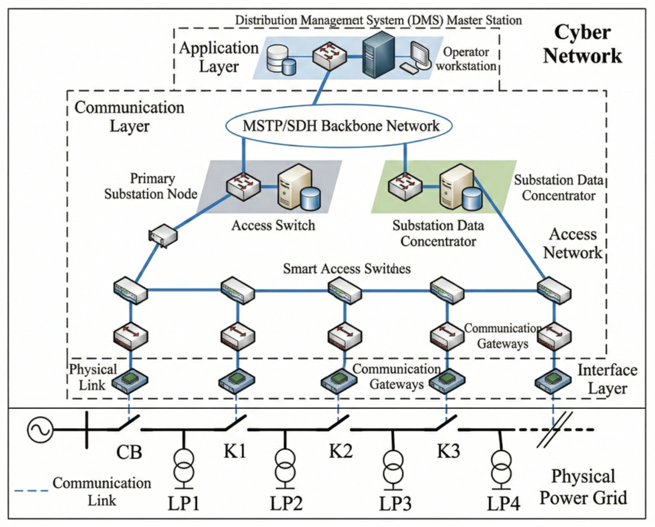
The cyber–physical distribution system model is illustrated in Figure 1. The information network is divided into three layers: the interface layer, the communication layer, and the application. The interface layer is mainly responsible for uploading monitoring data and executing control commands, and is typically composed of various intelligent electronic devices (IEDs). The communication layer consists of two parts: the backbone network and the access network. The backbone network connects the control center with substations and commonly adopts Synchronous Digital Hierarchy (SDH) and Multiservice Transport Platform (MSTP) technologies. The access network connects substations with IEDs and typically employs Ethernet Passive Optical Network (EPON) technology. Its typical structure consists of one Optical Line Terminal (OLT), multiple Optical Network Units (ONUs), and an Optical Distribution Network (ODN) equipped with Passive Optical Splitters (POS). The communication layer and the application layer together enable direct information exchange between terminal devices and the master station controller. In this paper, these components are collectively abstracted as communication nodes and communication links.

In the physical network shown in Figure 1, CB denotes a circuit breaker; $K_1$, $K_2$, and $K_3$ represent switches 1, 2, and 3, respectively; and $L{P}_1$, $L{P}_2$, $L{P}_3$, and $L{P}_4$ denote load points corresponding to specific electrical devices. In the proposed model, both the distribution network and the information network are represented using graph theory. Specifically, they are defined as $G_p(N_p,L_p)$ and $G_{IN}(N_{IN},L_{IN})$ respectively. Here, $N_p$ and $L_p$ denote the sets of buses and lines in the distribution network, respectively. Similarly, $N_{IN}$ and $L_{IN}$ represent the sets of communication nodes and communication links in the information network. The communication node set $N_{IN}$ can be further expressed as $N_{IN}=N_{\mathrm{OLT}}\cup N_{\mathrm{POS}}\cup N_{\mathrm{ONU}}$ In this formulation, $N_{\mathrm{OLT}}$ denotes the set of Optical Line Terminal (OLT) nodes, which are typically fiber termination devices deployed in substations or distribution stations. $N_{\mathrm{POS}}$ represents the set of Passive Optical Splitter (POS) nodes. Since POS devices are passive optical components that operate without external electrical power, their availability is independent of the distribution network’s power supply status. $N_{\mathrm{ONU}}$ and $N_{\mathrm{IED}}$ denote the sets of Optical Network Unit nodes and Intelligent Electronic Device nodes, respectively.

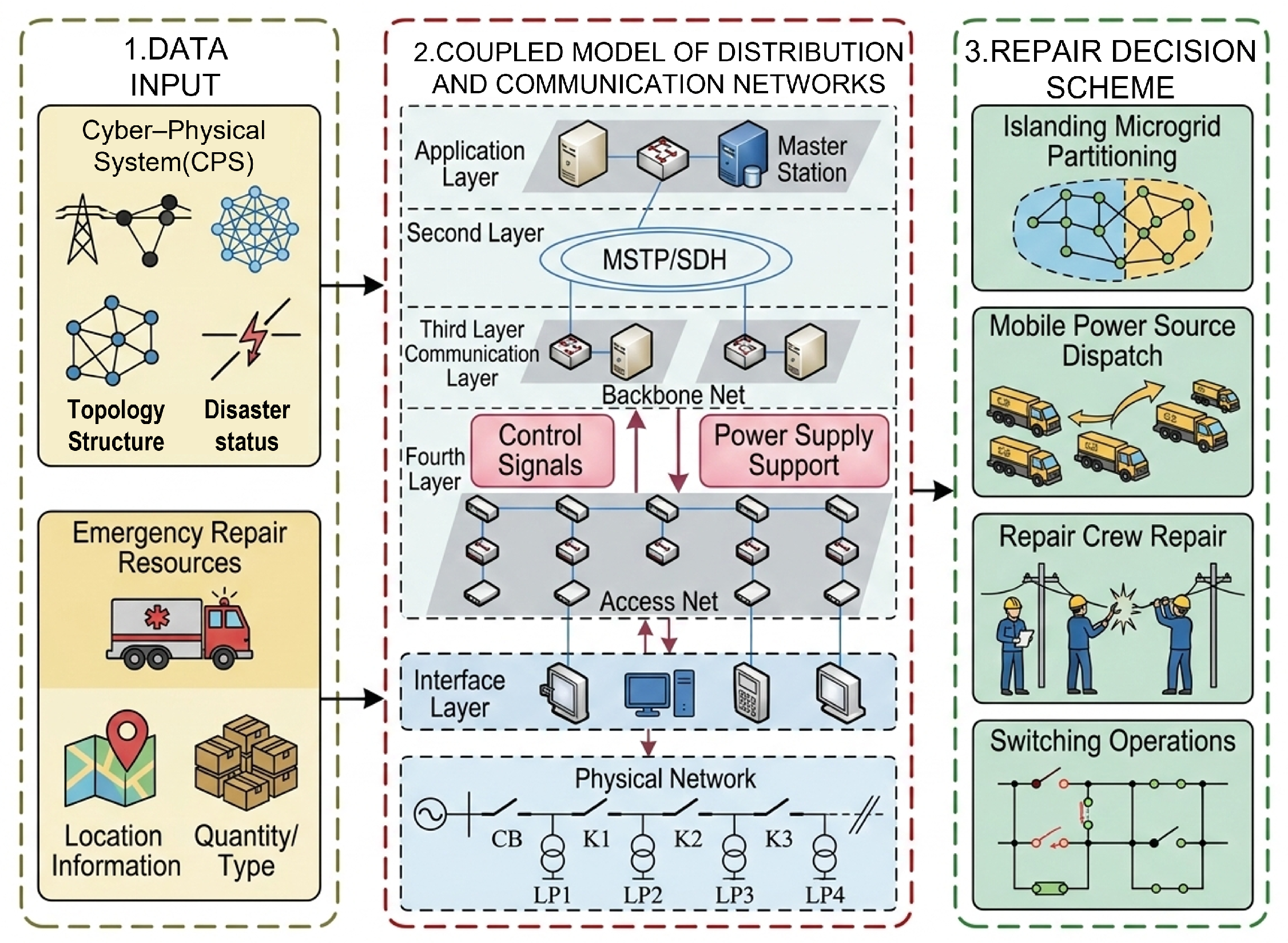
The distribution network primarily provides power supply support for intelligent devices in the communication network, whereas the communication network enables monitoring, control, and data transmission functions for the distribution network. When failures occur in communication network equipment, communication between intelligent terminal devices and the control center is interrupted, thereby reducing the controllability of the physical distribution network. When line faults occur in the distribution network and cause partial load outages, the corresponding communication nodes may also lose power supply. Without emergency backup power sources, distribution nodes may lose controllability. If faults occur simultaneously in both the distribution and communication networks, the severity of system outages is further aggravated. In such cases, not only must distribution lines be repaired, but communication network failures also require dedicated technical personnel for inspection and restoration. Therefore, based on the proposed coupling model and considering the topology and fault states of the cyber–physical distribution system, this study constructs a mobile emergency resource dispatch model and a joint repair model for the distribution and communication networks. These models support effective post-disaster repair decision-making. The overall research framework is illustrated in Figure 2.

3. Model for Coupled Distribution and Communication Networks

Existing emergency repair scheduling models for distribution networks typically assume fully functional communication systems capable of transmitting real-time operational information. However, extreme natural disasters may simultaneously disrupt both distribution and communication networks, impairing fault information exchange and reducing restoration efficiency. To address this limitation, this section develops a joint repair scheduling model that explicitly captures the cyber–physical coupling between the two networks. By integrating repair crew dispatch and mobile power allocation while accounting for the interdependent restoration processes of distribution and communication systems, the proposed model aims to enhance post-disaster recovery efficiency and overall system resilience.

3.1. Power–Communication Network Coupling Model

The coupling analysis between power distribution networks and communication networks is of critical importance, particularly under extreme disaster scenarios. The distribution network serves as the energy supply source for the communication network, while the communication network provides essential operational support for the reliable functioning of the power grid. Key components in power systems, such as substations, remotely controlled switches, and gas turbines, rely on communication networks for remote control and data exchange.

3.1.1. Communication Network Requirements for the Distribution Network

In cyber–physical distribution systems, communication routers depend on the power supply from the distribution network to transmit data and execute remote control commands. Therefore, the availability of communication router r at time t is modeled as

$$u_{r,t}\ge {\displaystyle \frac{P_{i\left(r\right),t}^{\mathrm{LD}}-P_{i\left(r\right),t}^{\mathrm{Shed}}-P_r}{M}},\forall t\in T$$

(1)

$$u_{r,t}\le M\left(P_{i\left(r\right),t}^{\mathrm{LD}}-P_{i\left(r\right),t}^{\mathrm{Shed}}-P_r\right),\forall t\in T$$

(2)

where r denotes the communication router index; $u_{r,t}$ is the availability status of router r at time t, taking value 1 if the router is connected and 0 otherwise; $i\left(r\right)$ denotes the node corresponding to router r; $P_{i\left(r\right),t}^{\mathrm{LD}}$ represents the maximum load demand at node $i\left(r\right)$ at time t; $P_{i\left(r\right),t}^{\mathrm{Shed}}$ denotes the load shedding amount at bus $i\left(r\right)$ at time t; $P_r$ is the power consumption of router r; and M is a sufficiently large constant used for big-M linearization.

3.1.2. Distribution Network Requirements for the Communication Network

In distribution systems, communication networks play a crucial role in enabling remote operation of switches, especially in the absence of centralized control at the main station. The operation of remote-controlled switches (RCSs) fully depends on communication routers and their coordinated functionality.

The operation of an RCS requires two necessary conditions: (i) the communication router connected to the RCS must be properly powered and free from communication link failures; (ii) all faults in the node cells associated with the RCS must be cleared.

Accordingly, the switching status of RCS s on line $l\left(s\right)$ at time t is modeled as

$$w_{l\left(s\right),t}^{\mathrm{RCS}}=\left\{\begin{array}{cc}1,\hfill & u_{r\left(s\right),t}=1\mathrm{and}(t-1)\Delta T\ge T_s^{\mathrm{NC},\mathrm{RCS}}+T_s^{\mathrm{RCSO}}\hfill \\ 0,\hfill & u_{r\left(s\right),t}=0\mathrm{or}(t-1)\Delta T<T_s^{\mathrm{NC},\mathrm{RCS}}+T_s^{\mathrm{RCSO}}\hfill \end{array}\right.$$

(3)

$$T_s^{\mathrm{NC},\mathrm{RCS}}=\underset{nc\in {\mathsf{\Omega }}_s^{\mathrm{NC},\mathrm{RCS}}}{max}{T}_{nc}^{\mathrm{NC}},\forall s\in {\mathsf{\Omega }}^{\mathrm{RCS}}$$

(4)

where $l\left(s\right)$ denotes the line associated with the s-th RCS; $w_{l\left(s\right),t}^{\mathrm{RCS}}$ is the switching status of the RCS, taking value 1 if the switch on line $l\left(s\right)$ is successfully closed at time t, and 0 otherwise; $r\left(s\right)$ denotes the communication router controlling the s-th RCS; $u_{r\left(s\right),t}$ is the availability of that router; $\Delta T$ is the dispatching time interval; $T_s^{\mathrm{NC},\mathrm{RCS}}$ is the maximum fault-clearing time among all node cells connected to RCS s; $T_s^{\mathrm{RCSO}}$ denotes the time required for remote switching operation; $T_{nc}^{\mathrm{NC}}$ is the fault-clearing time of node cell $nc$; ${\mathsf{\Omega }}_s^{\mathrm{NC},\mathrm{RCS}}$ is the set of node cells connected to RCS s; and ${\mathsf{\Omega }}^{\mathrm{RCS}}$ denotes the set of all RCSs.

The operation of RCSs is significantly influenced by the overall condition of the communication network. The connectivity and stability of the communication system determine whether RCSs can be operated in a timely and secure manner. If the communication network becomes unreliable, the automation and controllability of the distribution network will be severely constrained. Therefore, the tight coupling between communication and distribution networks is essential for enhancing operational efficiency and system stability.

3.2. Communication Network Model

In cyber–physical distribution systems, the availability of the communication network directly affects the control and dispatch of the distribution network, particularly the operation of remote-controlled switches and data transmission. To accurately characterize the availability of the communication system, this study models the working states of communication links through a routing-based formulation.

3.2.1. Communication Network Availability Model

The availability of the communication network is described by the operational states of routers and communication links, ensuring that the restored communication system can provide timely support to the distribution network after a disaster. The communication network availability model is formulated as

$$u_{r,k,t}^{\mathrm{Link}}\le {\displaystyle \frac{{\sum }_{r\in L_{r,k}}{u}_{r,t}}{n_{r,k}^{\mathrm{Link}}}},\forall k\in [1,n_r],\forall t\in T$$

(5)

$$u_{r,t}\le M\sum _{k=1}^{n_r}{u}_{r,k,t}^{\mathrm{Link}},\forall t\in T$$

(6)

where $\mathrm{Link}$ denotes the communication link of router r; $u_{r,k,t}^{\mathrm{Link}}$ represents the availability status of the k-th communication link of router r, taking value 1 if available at time t and 0 otherwise; $L_{r,k}$ is the set of routers included in the k-th communication link of router r; $u_{r,t}$ denotes the availability status of router r at time t; $n_{r,k}^{\mathrm{Link}}$ is the number of routers contained in the k-th communication link; $n_r$ is the total number of communication links of router r; and M is a sufficiently large constant.

Constraint (5) ensures that a communication link is considered connected only if all routers along that link are available. Specifically, $u_{r,k,t}^{\mathrm{Link}}=1$ only when every router on that link satisfies $u_{r,t}=1$. Constraint (6) guarantees that router r can operate effectively only if at least one communication link between the router and the control center remains connected.

3.2.2. Routing Constraints

If a communication path exists between network node i and the control center, two conditions must be satisfied: (i) the upstream node of i must maintain communication connectivity with the control center; (ii) node i must maintain a physical connection with its upstream node.

These routing constraints are expressed as follows:

$$v_{\mathrm{OLT},t}=1$$

(7)

$$v_{i,t}=v_{j,t},\forall j\in N_{\mathrm{IN}}\setminus N_F$$

(8)

$$v_{i,t}=v_{j,t}\wedge h_{ij,t},\forall j\in N_{\mathrm{IN}}\cap N_F$$

(9)

$${\mu }_{i,t}=v_{i,t}\wedge {\delta }_{i,t},\forall i\in N_{\mathrm{ONU}}$$

(10)

$${\mu }_{i,t}=v_{i,t},\forall i\in N_{\mathrm{POS}}$$

(11)

where $v_{\mathrm{OLT},t}$ denotes the link status between the OLT node and the control center; $v_{i,t}$ represents the connectivity status between node i and the control center (equal to 1 if a physical communication path exists, and 0 otherwise); $h_{ij,t}$ denotes the repair status of communication line $ij$ (equal to 1 if repaired at time t, and 0 otherwise); $N_F$ is the set of failed components; ${\delta }_{i,t}$ indicates the power supply status of node i at time t (equal to 1 if sufficiently powered, and 0 otherwise); and ${\mu }_{i,t}$ denotes the communication availability status of node i.

Constraint (7) specifies that the OLT node is always connected to the control center, as it is protected in the backbone network and assumed not to fail. Constraint (8) indicates that if node i and its upstream node j are both functional, the connectivity of node i depends on the state of node j. Constraint (9) further ensures that the connectivity of node i depends not only on the upstream node state but also on whether the communication line between them has been repaired. Constraint (10) states that an IED/ONU node can establish communication only when a physical path exists and sufficient power supply is available. Constraint (11) specifies that the communication status of POS nodes depends solely on connectivity, since POS devices are passive components and do not require external power supply. Since POS devices are passive optical components that operate without external electrical power, their availability is independent of the distribution network’s power supply status. Nevertheless, POS nodes may still fail due to physical damage, which is reflected in their communication status depending solely on whether a physical path exists between communication node and the control center, as captured by Equations (7)–(11).

3.3. Distribution Network Model

When extreme disasters cause power outages in distribution networks, repair crews are dispatched to restore faulted lines and mobile power sources are connected to critical nodes. Substations or black-start power units are taken as the starting points of restoration paths to recover interrupted loads. Accordingly, a distribution network restoration model incorporating restoration paths and operational constraints is formulated.

3.3.1. Restoration Path Modeling

During the restoration process, both line repair and mobile power integration are considered. The restoration path originates from grid-forming devices, and is modeled as follows:

$$p_{i,i,t}\le 1,\forall i\in GF,\forall t$$

(12)

$$p_{i,i,t}=0,\forall i\notin GF$$

(13)

$$\sum _{j\in V}{p}_{j,i,t}\le \sum _{j\in V}{p}_{i,j,t},\forall i,\forall t$$

(14)

$$p_{i,j,t}+p_{j,i,t}\le {\beta }_{i,j,t},\forall (i,j),\forall t$$

(15)

$${\beta }_{i,j,t}\le s_{i,j,t},\forall (i,j),\forall t$$

(16)

$$\sum _{j\in V}{p}_{j,i,t}\ge u_{k,i,t},\forall i\notin BDG,\forall t$$

(17)

$$\sum _{i\in V}{p}_{i,j,t}\le 1,\forall j,\forall t$$

(18)

where $p_{i,j,t}$ denotes the restoration path between nodes i and j at time t; $GF$ is the set of grid-forming nodes; ${\beta }_{i,j,t}$ represents the switching status of line $(i,j)$; V is the set of all distribution network nodes; $s_{i,j,t}$ is the repair status of line $(i,j)$; $u_{k,i,t}$ denotes the restoration status of node i; and $BDG$ represents black-start generator nodes.

Constraints (12)–(13) ensure that restoration paths originate only from grid-forming devices. Constraint (14) guarantees that a node can transmit restoration power only if it has an incoming restoration path. Constraint (15) ensures that at most one restoration direction is selected on a closed line. Constraint (16) prevents restoration paths from being established on unrepaired lines. Constraint (17) states that a node can be restored only if it is connected by a restoration path. Constraint (18) enforces radial restoration topology.

3.3.2. Distribution Network Operational Model

The operational model simulates and optimizes power transmission and distribution to ensure stable and efficient operation during restoration. It includes distributed generation outputs, line power flows, and nodal voltage constraints [25].

$$0\le P{D}_{i,t}\le u_{i,t}^{DY}P{L}_i,\forall t,\forall i$$

(19)

$$0\le P{G}_{i,t}\le u_{i,t}^{DN}P{G}_i^{max},\forall t,\forall i$$

(20)

$$0\le Q{G}_{i,t}\le u_{i,t}^{DN}Q{G}_i^{max},\forall t,\forall i$$

(21)

$$0\le P{G}_{i,t}^m\le u_{i,t}^{DN}P{G}_i^{m,max},\forall t,\forall i$$

(22)

$$0\le Q{G}_{i,t}^m\le u_{i,t}^{DN}Q{G}_i^{m,max},\forall t,\forall i$$

(23)

$$-M{P}_{i,j,t}\le P_{i,j,t}\le M{P}_{i,j,t},\forall (i,j),\forall t$$

(24)

$$-M{P}_{i,j,t}\le Q_{i,j,t}\le M{P}_{i,j,t},\forall (i,j),\forall t$$

(25)

$$\sum _{j\in V}{P}_{j,i,t}+P{G}_{i,t}+P{G}_{i,t}^m+P_{i,t}^{wind}=P{D}_{i,t}+\sum _{j\in V}{P}_{i,j,t},\forall i,\forall t$$

(26)

$$\sum _{j\in V}{Q}_{j,i,t}+Q{G}_{i,t}+Q{G}_{i,t}^m=Q{D}_{i,t}+\sum _{j\in V}{Q}_{i,j,t},\forall i,\forall t$$

(27)

$$U_{i,t}-U_{j,t}\le 2(R_{i,j}{P}_{i,j,t}+X_{i,j}{Q}_{i,j,t})+M(1-x_{i,j,t}),\forall (i,j),\forall t$$

(28)

$$U_{i,t}-U_{j,t}\ge 2(R_{i,j}{P}_{i,j,t}+X_{i,j}{Q}_{i,j,t})-M(1-x_{i,j,t}),\forall (i,j),\forall t$$

(29)

$$u_{i,t}{\underline{U}}_i\le U_{i,t}\le u_{i,t}{\overline{U}}_i,\forall i,\forall t$$

(30)

where $P{D}_{i,t}$ denotes restored load; $P{L}_i$ is load demand; $u_{i,t}^{DY}$ and $u_{i,t}^{DN}$ denote load and generator operational states; $P{G}_{i,t}$, $Q{G}_{i,t}$ are active/reactive outputs of distributed generators; $P{G}_{i,t}^m$, $Q{G}_{i,t}^m$ are outputs of mobile power units; $P_{i,j,t}$ and $Q_{i,j,t}$ denote line power flows; $P_{i,t}^{wind}$ is wind generation output; $R_{i,j}$ and $X_{i,j}$ are line resistance and reactance; $U_{i,t}$ is nodal voltage; ${\underline{U}}_i$ and ${\overline{U}}_i$ are voltage limits; and $x_{i,j,t}$ is the repair status of line $(i,j)$.

Constraints (19)–(23) define load recovery and generation limits. Constraints (24)–(25) bound line power flows. Constraints (26)–(27) enforce nodal active and reactive power balance. Constraints (28)–(29) represent voltage drop relations. Constraint (30) ensures nodal voltage limits.

3.4. Repair Crew Deployment and Scheduling Model

The repair crew dispatching of communication and distribution networks is a critical component of emergency management. The objective is to optimally allocate and utilize repair resources to minimize fault recovery time. Under large-scale outages caused by extreme disasters, multiple repair crews must be scheduled. Based on fault priority, network coupling relationships, and spatial distance, repair routes and service sequences are determined to enhance restoration efficiency.

Notably, the restoration status of the communication network directly affects the repair sequence of the distribution network. When communication failures occur, crew dispatching must consider the timing of communication recovery and regional coverage. Conversely, the progress of distribution network restoration may influence communication traffic loads, thereby affecting communication recovery strategies. Therefore, the repair crew scheduling model comprehensively considers fault locations and resource availability to ensure rapid restoration of both communication and distribution networks.

The repair crew deployment and scheduling model is formulated as follows:

$$\sum _{c\in C}{x}_{W,i}^c=1,\forall c$$

(31)

$$\sum _W{x}_{W,i}^c\le N_c,\forall c$$

(32)

$$\sum _{i\in {\mathsf{\Phi }}_F}{x}_{W,i}^c=1,\forall c$$

(33)

$$\sum _{i\in {\mathsf{\Phi }}_F}{x}_{i,W}^c=1,\forall c$$

(34)

$$\sum _{j\in {\mathsf{\Phi }}_F}{x}_{j,i}^c-\sum _{e\in {\mathsf{\Phi }}_F}{x}_{i,e}^c=0,\forall c,\forall i$$

(35)

$$y_i^c=\sum _{j\in {\mathsf{\Phi }}_F}{x}_{j,i}^c,\forall c,\forall i$$

(36)

$$\sum _{c\in {\mathsf{\Phi }}_R}{y}_i^c\le 1,\forall i$$

(37)

$$\sum _{t\in T}{f}_{i,t}^c\le 1,\forall i$$

(38)

$$\sum _{t\in T}t·f_{i,t}^c=\sum _{c\in {\mathsf{\Phi }}_R}{T}_i^c+\sum _{c\in {\mathsf{\Phi }}_R}re{p}_i^c{y}_i^c,\forall i$$

(39)

$$s_i^c=\sum _{\tau =1}^{t-1}{f}_{i,\tau }^c,\forall i$$

(40)

where ${\mathsf{\Phi }}_F$ denotes the set of all fault nodes; i, j, and e are node indices in either the communication or distribution network; W represents the depot node of repair crews. Each repair crew departs from the depot and returns after completing assigned tasks. $x_{W,i}^c$ equals 1 if repair crew c travels from depot W to fault node i, and 0 otherwise. Similarly, $x_{i,W}^c$ equals 1 if crew c returns from fault node i to depot W. The binary variable $x_{i,j}^c$ indicates whether crew c travels from fault node i to fault node j. ${\mathsf{\Phi }}_R$ represents the set of repair crews; $y_i^c$ equals 1 if fault node i is repaired by crew c, and 0 otherwise. T is the set of repair time periods; $T_i^c$ denotes the travel time required for crew c to reach fault node i; $f_{i,t}^c$ is a binary variable indicating whether crew c is working at fault node i at time t; $re{p}_i^c$ denotes the repair time required by crew c at fault node i; and $s_i^c$ indicates whether fault node i has been repaired by crew c.

Constraints (31)–(32) ensure that at most one repair crew can be deployed at each depot, and that the total number of deployed crews does not exceed the prescribed upper limit. Constraints (33)–(34) ensure that each repair crew departs from and returns to the depot, forming a closed tour. Constraint (35) guarantees flow conservation at each fault node, maintaining route continuity. Constraints (36)–(37) restrict each fault node to be repaired by at most one repair crew, avoiding redundant work. Constraint (38) ensures that a fault node cannot be repaired simultaneously by multiple crews. Constraint (39) links the actual repair completion time to the crew arrival time and repair duration, ensuring temporal consistency. Constraint (40) defines the repair status of each fault node.

To further capture the coupling between communication recovery and repair crew scheduling, the following constraints are introduced. Since fault information of a distribution node can only be obtained after the corresponding communication node is restored, repair crews are permitted to commence work at a fault node only after its observability has been established. The fault information observability constraint is given by:

$$\begin{array}{cc}\hfill & f_{i,t}^c\le {\mu }_{i\left(f\right),t},\forall i\in {\mathsf{\Phi }}_F,\forall c\in {\mathsf{\Phi }}_R,\forall t\in T\hfill \end{array}$$

(41)

$$\begin{array}{cc}\hfill & T_i^{\mathrm{comm},\mathrm{restore}}=\sum _{t\in T}t·\left({\mu }_{i\left(f\right),t}-{\mu }_{i\left(f\right),t-1}\right),{\mu }_{i\left(f\right),0}=0\hfill \end{array}$$

(42)

$$\begin{array}{cc}\hfill & x_{i,j}^c\le {\mu }_{j\left(f\right),t_{\mathrm{arrive}}^{c,j}},\forall (i,j)\in {\mathsf{\Phi }}_F\times {\mathsf{\Phi }}_F,\forall c\in {\mathsf{\Phi }}_R\hfill \end{array}$$

(43)

where ${\mu }_{i\left(f\right),t}$ denotes the communication availability status of the communication node corresponding to fault node i at time t; $T_i^{\mathrm{comm},\mathrm{restore}}$ denotes the communication restoration time of fault node i. Constraint (41) ensures that a repair crew can work at fault node i at time t only if the associated communication node has already been restored. Constraint (42) defines the moment at which the communication node first becomes available. Constraint (43) ensures that crew c may travel from node i to node j only if the communication node corresponding to fault node j has been restored by the time the crew would arrive, thereby tightly coupling the communication restoration sequence with the distribution repair schedule.

To guarantee that the resulting repair routes are physically continuous, non-branching, and non-instantaneous, the MTZ subtour elimination constraints and continuous-time linking constraints are incorporated as follows:

$$\begin{array}{cc}\hfill & {\eta }_j^c-{\eta }_i^c\ge 1-\left|{\mathsf{\Phi }}_F\right|\left(1-x_{i,j}^c\right),\forall i,j\in {\mathsf{\Phi }}_F,i\ne j,\forall c\in {\mathsf{\Phi }}_R\hfill \end{array}$$

(44)

$$\begin{array}{cc}\hfill & 1\le {\eta }_i^c\le \left|{\mathsf{\Phi }}_F\right|,\forall i\in {\mathsf{\Phi }}_F,\forall c\in {\mathsf{\Phi }}_R\hfill \end{array}$$

(45)

$$\begin{array}{cc}\hfill & A{T}_j^c\ge A{T}_i^c+re{p}_i^c+{\tau }_{i,j}^{\mathrm{travel}}-M\left(1-x_{i,j}^c\right),\forall i,j\in {\mathsf{\Phi }}_F,\forall c\in {\mathsf{\Phi }}_R\hfill \end{array}$$

(46)

$$\begin{array}{cc}\hfill & A{T}_i^c\ge {\tau }_{d,i}^{\mathrm{travel}}·x_{d,i}^c,\forall i\in {\mathsf{\Phi }}_F,\forall c\in {\mathsf{\Phi }}_R\hfill \end{array}$$

(47)

$$\begin{array}{cc}\hfill & D{T}_i^c=A{T}_i^c+re{p}_i^c,\forall i\in {\mathsf{\Phi }}_F,\forall c\in {\mathsf{\Phi }}_R\hfill \end{array}$$

(48)

$$\begin{array}{cc}\hfill & A{T}_j^c-D{T}_i^c\ge {\tau }_{i,j}^{\mathrm{travel}}-M\left(1-x_{i,j}^c\right),\forall (i,j),\forall c\in {\mathsf{\Phi }}_R\hfill \end{array}$$

(49)

where ${\eta }_i^c$ denotes the visiting order of repair crew c at fault node i; $A{T}_i^c$ and $D{T}_i^c$ denote the arrival and departure times of repair crew c at fault node i, respectively; ${\tau }_{i,j}^{\mathrm{travel}}$ is the physical travel time from node i to node j; ${\tau }_{d,i}^{\mathrm{travel}}$ is the travel time from depot d to node i; and M is a sufficiently large constant. When $x_{i,j}^c=1$, Constraint (44) enforces ${\eta }_j^c\ge {\eta }_i^c+1$, thereby eliminating subtours and ensuring a strictly sequential visiting order. Constraint (46) links the arrival times of consecutive fault nodes, incorporating both the repair duration and travel time. Constraint (47) ensures a valid initial arrival time from the depot. Constraint (48) defines the departure time at each node, and Constraint (49) enforces the physical travel time between successive nodes. Constraints (44)–(49) collectively guarantee that each crew follows a physically realizable, continuous, and non-overlapping repair route with no instantaneous transitions between non-adjacent locations.

3.5. Mobile Power Source Deployment and Dispatch Model

When both distribution and communication networks experience failures due to disasters, certain loads may lose power supply. In such cases, mobile power units should be optimally allocated and routed to support critical loads. The mobile power dispatch model determines the allocation and routing of mobile power units through an optimization framework, aiming to maximize restoration efficiency and service coverage, thereby reducing the economic and social impacts of outages and enhancing post-disaster emergency response capability and system resilience.

The proposed mobile power dispatch model is formulated as follows:

$$\sum _{m\in M}{z}_{d,i}^m=1,\forall m$$

(50)

$$\sum _d{z}_{d,i}^m=1\le N_m,\forall m$$

(51)

$$\sum _{i\in {\mathsf{\Phi }}_F}{z}_{d,i}^m=1,\forall m$$

(52)

$$\sum _{j\in {\mathsf{\Phi }}_F}{z}_{j,i}^m-\sum _{e\in {\mathsf{\Phi }}_F}{z}_{i,e}^m=0,\forall m,\forall i$$

(53)

$$\sum _{t\in T}{f}_{i,t}^F\le 1,\forall i$$

(54)

$$\sum _{t\in T}t{f}_{i,t}^F=\sum _{m\in {\mathsf{\Phi }}_F}A{T}_i^m,\forall i$$

(55)

$$\sum _{t\in T}{o}_{i,t}^m\le 1,\forall i$$

(56)

$$\sum _{t\in T}t{o}_{i,t}^m=\sum _{m\in {\mathsf{\Phi }}_F}{T}_i^m+\sum _{m\in {\mathsf{\Phi }}_F}{g}_i^m,\forall i$$

(57)

$$s_i=\sum _{\tau =1}^{t-1}{f}_{i,\tau }^F-\sum _{\tau =1}^{t-1}{o}_{i,\tau }^m,\forall i$$

(58)

where $z_{i,j}^m$ represents the routing decision of mobile power unit m from node i to node j; d denotes the initial depot location of mobile power units; $T_i^m$ represents the travel time required for mobile power unit m to reach node i; $f_{i,t}^F$ indicates whether fault node i is supplied with power at time t; $o_{i,t}^m$ denotes whether mobile power unit m departs from node i at time t; $g_i^m$ represents the duration for connecting mobile power unit m to node i; and $s_i$ denotes the power supply status of fault node i.

Constraints (50) and (51) are imposed to ensure that at most one mobile energy storage unit can be deployed at each location, and that the total number of deployed units does not exceed the prescribed upper limit. The constraint (52) ensures that each mobile power unit begins its dispatch process from its initial location. The second constraint guarantees flow conservation, ensuring that once a mobile power unit arrives at a fault node, it must depart to another node to maintain supply continuity. Constraints (53)–(58) determine the arrival and departure times of mobile power units at each connection node to coordinate power supply operations. The final constraint defines the supply status of fault node i.

3.6. Objective Functions

When extreme disasters simultaneously disrupt both communication and distribution networks, leading to large-scale outages, the pre-disaster deployment model aims to minimize the expected load loss across all possible disaster scenarios. The objective function is formulated as

$$\min \sum _{s\in \mathcal{S}}{\pi }_s\sum _{i\in N_p\cup N_{IN}}\sum _{t\in T}\rho \left(P{L}_{i,t}^s-P{D}_{i,t}^s\right)$$

(59)

where ${\pi }_s$ denotes the probability of disaster scenario s.

The post-disaster restoration model considers a deterministic disaster scenario and aims to minimize the load loss of the distribution network under that specific condition. The objective function is expressed as

$$\min \sum _{i\in N_p\cup N_{IN}}\sum _{t\in T}\rho \left(P{L}_{i,t}-P{D}_{i,t}\right).$$

(60)

In the above formulation, $\rho$ denotes the load weighting factor in the distribution network. The objective essentially minimizes the difference between the load demand and the restored load (i.e., the load loss), which is used to evaluate and optimize the effectiveness of the repair and restoration strategy.

Subject to the mobile emergency resource dispatch constraints and coupled repair constraints of the distribution and communication networks, the proposed model minimizes distribution-level load loss and yields the corresponding emergency resource scheduling plan and post-disaster repair and restoration results.

4. Framework and Solution Method

4.1. Two-Stage Optimization Framework

To enhance the resilience of coupled distribution–communication systems under extreme disasters, a two-stage optimization framework is established to coordinate pre-disaster resource deployment and post-disaster restoration decisions.

In the first stage, a pre-disaster deployment model is formulated to determine the optimal allocation and initial locations of emergency resources, including repair crews and mobile power sources, before the disaster occurs. The objective function of the first stage aims to minimize the expected restoration loss under multiple disaster scenarios, as expressed in (59). The constraints associated with the pre-disaster deployment stage mainly include the constraints (1)–(58). These constraints jointly describe the structural and operational relationships between the distribution network and the communication network, as well as the availability and scheduling feasibility of emergency repair resources.

In the second stage, a post-disaster restoration model is constructed to determine the optimal repair scheduling, network reconfiguration, and mobile power dispatch after the disaster realization. The objective function of the restoration stage is to minimize load shedding and restoration losses during the recovery horizon, as defined in (60). The constraints associated with the pre-disaster deployment stage mainly include the constraints (1)–(30) and constraints (35)–(58). These constraints ensure the secure operation of the distribution network while coordinating repair and restoration activities in the coupled cyber–physical infrastructure.

Since several constraints in the original formulation contain nonlinear relationships, such as the power flow equations and logical coupling relations between binary and continuous variables, linearization techniques are required to transform the model into a tractable optimization form. In this study, the nonlinear terms are linearized using standard techniques including Big-M linearization and piecewise linear approximation, thereby converting the overall model into a MILP formulation

For the structure appearing in Equation (3), the following linearization is adopted.

$$\begin{array}{cc}\hfill & w_{l\left(s\right),t}^{\mathrm{RCS}}\le u_{r\left(s\right),t}\hfill \\ \hfill & w_{l\left(s\right),t}^{\mathrm{RCS}}\le {\displaystyle \frac{(t-1)\Delta T-T_s^{\mathrm{NC},\mathrm{RCS}}-T_s^{\mathrm{RCSO}}}{M}}+1\hfill \\ \hfill & w_{l\left(s\right),t}^{\mathrm{RCS}}\ge u_{r\left(s\right),t}+{\displaystyle \frac{(t-1)\Delta T-T_s^{\mathrm{NC},\mathrm{RCS}}-T_s^{\mathrm{RCSO}}}{M}}-1\hfill \end{array}$$

(61)

For the structure appearing in Equation (4), the following linearization is adopted.

$$\begin{array}{cc}\hfill & T_s^{\mathrm{NC},\mathrm{RCS}}\ge T_{nc}^{\mathrm{NC}}\forall nc\in {\mathsf{\Omega }}_s^{\mathrm{NC},\mathrm{RCS}}\hfill \\ \hfill & T_s^{\mathrm{NC},\mathrm{RCS}}\le T_{nc}^{\mathrm{NC}}+M(1-{\alpha }_{nc})\forall nc\in {\mathsf{\Omega }}_s^{\mathrm{NC},\mathrm{RCS}}\hfill \\ \hfill & \sum _{nc}{\alpha }_{nc}=1\hfill \end{array}$$

(62)

For the structures appearing in Equations (9), the following linearization is adopted.

$$\begin{array}{cc}\hfill & v_{i,t}\le v_{j,t}\hfill \\ \hfill & v_{i,t}\le h_{j,i,t}\hfill \\ \hfill & v_{i,t}\ge v_{j,t}+h_{j,i,t}-1\hfill \end{array}$$

(63)

4.2. Solution Methodology

The proposed pre-disaster deployment approach embeds the post-disaster restoration model into the pre-disaster planning framework, thereby enabling the evaluation of potential recovery performance under anticipated disaster scenarios. Accordingly, the pre-disaster deployment model utilizes disaster early-warning information to determine the optimal pre-positioning strategy of emergency recovery resources. The specific solution procedure is summarized as follows:

(1) Disaster early-warning information is collected, and component failure scenarios are generated based on historical data and Monte Carlo simulation.

(2) The generated disaster scenarios are incorporated into Equations (1)–(58) to formulate the two-stage optimization model.

(3) The resulting model is solved using a Progressive Hedging (PH) algorithm framework that accounts for mixed-integer resource allocation decisions, ultimately yielding the optimal pre-disaster deployment strategy for recovery resources.

Disaster scenarios are generated based on historical typhoon fragility data using Monte Carlo simulation, yielding $\left|S\right|=100$ candidate disaster scenarios with associated occurrence probabilities ${\pi }_s$ estimated from historical frequencies. To balance computational efficiency and solution quality, a forward-selection method is subsequently applied to reduce the scenario set to $\left|S\right|=10$ representative scenarios for use in the Progressive Hedging decomposition framework.

The pre-disaster deployment model embeds the post-disaster restoration model into the pre-disaster planning framework, enabling the evaluation of potential recovery performance under anticipated disaster scenarios. The PH algorithm decomposes the two-stage stochastic program into per-scenario subproblems that are solved iteratively to enforce non-anticipativity. The post-disaster restoration problem is solved based on the realized damage scenario. The detailed PH procedure is summarized in Algorithm 1.

Algorithm 1 Form of the progressive hedging algorithm applied to the pre-disaster deployment model

Optimization We confirm that this table does not contain a table header. problem ${\displaystyle \min (\chi ·\xi )+\sum _{s\in S}{\pi }_s({\varphi }_s·{\psi }_s)}$

${\displaystyle \mathrm{s}.\mathrm{t}.(\xi ,{\psi }_s)\in {\mathsf{\Theta }}_s}$

No. Progressive hedging procedure

1 ${\displaystyle k:=0,{\omega }_s^{\left(k\right)}:=0}$, given tolerance $\epsilon ={10}^{-3}$ and initial penalty parameter ${\rho }_0$.

2 For all scenarios $s\in S$, compute ${\displaystyle {\xi }_s^{\left(k\right)}:=\arg \underset{\xi ,{\psi }_s}{\min }\left\{\chi ·\xi +{\varphi }_s·{\psi }_s:(\xi ,{\psi }_s)\in {\mathsf{\Theta }}_s\right\}.}$

3 Compute the weighted consensus: ${\displaystyle {\overline{\xi }}^{\left(k\right)}:=\sum _{s\in S}{\pi }_s{\xi }_s^{\left(k\right)}.}$

4 For all scenarios $s\in S$, update multipliers: ${\displaystyle {\omega }_s^{\left(k\right)}:=\rho \left({\xi }_s^{\left(k\right)}-{\overline{\xi }}^{\left(k\right)}\right).}$

5 Update iteration counter: ${\displaystyle k:=k+1}$.

6 For all scenarios $s\in S$, solve the augmented subproblem:   ${\displaystyle {\xi }_s^{\left(k\right)}:=\arg \underset{\xi ,{\psi }_s}{\min }\left\{\chi ·\xi +{\omega }_s^{(k-1)}·\xi +\frac{\rho }{2}{∥\xi -{\overline{\xi }}^{(k-1)}∥}_2^2+{\varphi }_s·{\psi }_s:(\xi ,{\psi }_s)\in {\mathsf{\Theta }}_s\right\}.}$

7 Update the weighted consensus: ${\displaystyle {\overline{\xi }}^{\left(k\right)}:=\sum _{s\in S}{\pi }_s{\xi }_s^{\left(k\right)}.}$

8 For all scenarios $s\in S$, update multipliers: ${\displaystyle {\omega }_s^{\left(k\right)}:=\rho \left({\xi }_s^{\left(k\right)}-{\overline{\xi }}^{\left(k\right)}\right).}$

9 Adaptive penalty update: if ${\gamma }^{\left(k\right)}$ decreases by less than 10% over 5 consecutive iterations, set $\rho :=\min (1.2\rho ,10{\rho }_0)$.

10  Compute the convergence metric: ${\displaystyle {\gamma }^{\left(k\right)}:=\sum _{s\in S}{\pi }_s{∥{\xi }_s^{\left(k\right)}-{\overline{\xi }}^{\left(k\right)}∥}_2.}$

11 If ${\displaystyle {\gamma }^{\left(k\right)}\ge \epsilon }$, go to Step 5; otherwise, terminate.

The first-stage decision vector $\xi$ represents the pre-disaster deployment decisions of repair crews and mobile power sources before any disaster scenario is revealed: $\xi =\{N_c^s,N_m^s,lo{c}_c,lo{c}_m\}$, $N_c^s$ and $N_m^s$ denote the numbers of each resource type, and $lo{c}_c$, $lo{c}_m$ denote their initial deployment locations. These decisions must be made prior to scenario realization and are therefore required to satisfy non-anticipativity constraints across all scenarios $s\in S$.

The second-stage decision vector ${\psi }_s$ captures the post-disaster dispatch decisions, including: repair crew routing $x_{i,j}^{c,s}$, mobile power source routing $z_{i,j}^{m,s}$, network switch operations ${\beta }_{i,j,t}^s$, load restoration $P{D}_{i,t}^s$, and the associated timing variables $A{T}_i^{c,s}$, $D{T}_i^{c,s}$.

The two stages are coupled through resource availability constraints: in any scenario s, the number of dispatchable repair crews and mobile power sources cannot exceed the pre-deployed quantities $\xi$ determined in the first stage. Non-anticipativity is enforced within the PH framework via an augmented Lagrangian penalty:

$${\omega }_s^{\left(k\right)}·{\xi }_s+{\displaystyle \frac{\rho }{2}}{∥{\xi }_s-{\overline{\xi }}^{\left(k\right)}∥}_2^2.$$

(64)

Each scenario subproblem is formulated as a Mixed-Integer Linear Program and solved independently using Gurobi 11.0 through MATLAB R2024a.

The use of an arbitrarily large Big-M value can cause numerical instability and weaken the LP relaxation. To address this concern, problem-specific, tight upper bounds are derived for every occurrence of M in the proposed formulation, as summarised in

Table 1. Tight Big-M values used in the proposed formulation.

Eq.	Role of M	Bound and Value Used
(1) and (2)	Bounds net nodal power.	$M\ge {max}_{i,t}{P}_{i,t}^{\mathrm{LD}}$; total system demand of the IEEE 33-bus network: $M=3710\mathrm{kW}$.
(6)	Bounds available communication links.	$M\ge n_r^{max}$; maximum links per router in the test network: $M=4$.
(28) and (29)	Relaxes voltage-drop equality on open lines.	$M\ge (\overline{U}-\underline{U})+2{max}_{(i,j)}(R_{ij}{P}_{ij}^{max}+X_{ij}{Q}_{ij}^{max})$; with $[\underline{U},\overline{U}]=[0.81,1.21]\mathrm{p}.\mathrm{u}{.}^2$: $M=1.0\mathrm{p}.\mathrm{u}{.}^2$.
(44) and (45)	MTZ subtour elimination.	$M\ge |{\mathsf{\Phi }}_F|$; worst-case fault count: $M=8$.
(46)–(49)	Links consecutive arrival times.	$M\ge T_{\mathrm{horizon}}+maxre{p}_i^c+max{\tau }_{ij}^{\mathrm{travel}}$; $M=12\mathrm{h}$.
(61)	Bounds discrete time index.	$M=T_{\mathrm{horizon}}/\Delta T=30$ time steps.
(62) and (63)	Linearises binary coupling terms.	$M=10\mathrm{h}$ for temporal terms; $M=1$ for binary terms.

.

These problem-specific bounds keep M as tight as the physical system allows. All M values are likewise derived from physical or combinatorial upper bounds rather than from an arbitrary large number, thereby preserving LP-relaxation tightness and numerical stability.

5. Case Study

In this section, an enhanced IEEE 33-bus cyber–physical distribution network is adopted to validate the effectiveness of the proposed coordinated repair and restoration strategy under coupled cyber–physical failure conditions. Each installed distributed generation (DG) unit has a rated capacity of 100 kW. In the test system, all tie switches are initially set to open, while the remaining sectionalizing switches are set to closed. The repair time for each faulted component is assumed to be 1 h. The simulation time step is 20 min. The mobile power source is modeled as a mobile diesel generator unit with rated capacity 200 kW, maximum reactive power output 100 kvar, connection/disconnection time 0.5 h, and sufficient fuel capacity for the entire restoration horizon. The travel time between locations is calculated based on the distance between nodes. It is assumed that repair crews are specialized by professional category, with one dedicated crew assigned to the communication network and one to the distribution network, respectively. Due to differences in technical expertise and operational requirements, each crew is restricted to servicing its corresponding network. All experiments are conducted on a workstation equipped with an Intel Core i7-14700HX CPU and 32 GB RAM. The optimization model is implemented in Python 3.10 and solved using Gurobi 11.0. The computational time for simulation is 2540.32 s. The base voltage of the IEEE 33-bus test system is 12.66 kV, and the total load demand is 3.71 MW + 1.50 Mvar. The travel time between locations is calculated based on the Euclidean distances between nodes in the IEEE 33-bus test system, following the distance-based travel time modeling approach adopted in [26]. Specifically, the travel time between nodes i and j is computed as ${\tau }_{i,j}^{\mathrm{travel}}=d_{i,j}/v$, where $d_{i,j}$ is the straight-line distance derived from the node coordinates and v is the assumed constant travel speed of repair crews and mobile power sources.

The worst-case damage scenario is defined as follows: distribution lines D2-3, D15-16, D2-19, D29-30, and D32-33 are damaged. Since distribution lines and communication cables are installed in parallel along the same corridors, extreme disasters are likely to cause simultaneous failures. Accordingly, the corresponding communication cables C2-3, C15-16, C2-19, C29-30, and C32-33 are also assumed to be out of service.

Typhoon Yagi is used as a representative motivating example due to its well-documented impact on distribution infrastructure in 2024. It should be noted that the proposed framework is disaster-agnostic, since disaster effects are represented through component failure states rather than disaster-specific physical processes. For other disaster types such as floods, earthquakes, or ice storms, only the scenario generation stage needs to be adjusted via appropriate fragility models, while the optimization model and solution method remain unchanged.

5.1. Comparative Analysis of Different Methods

5.1.1. Deployment and Restoration Process Analysis

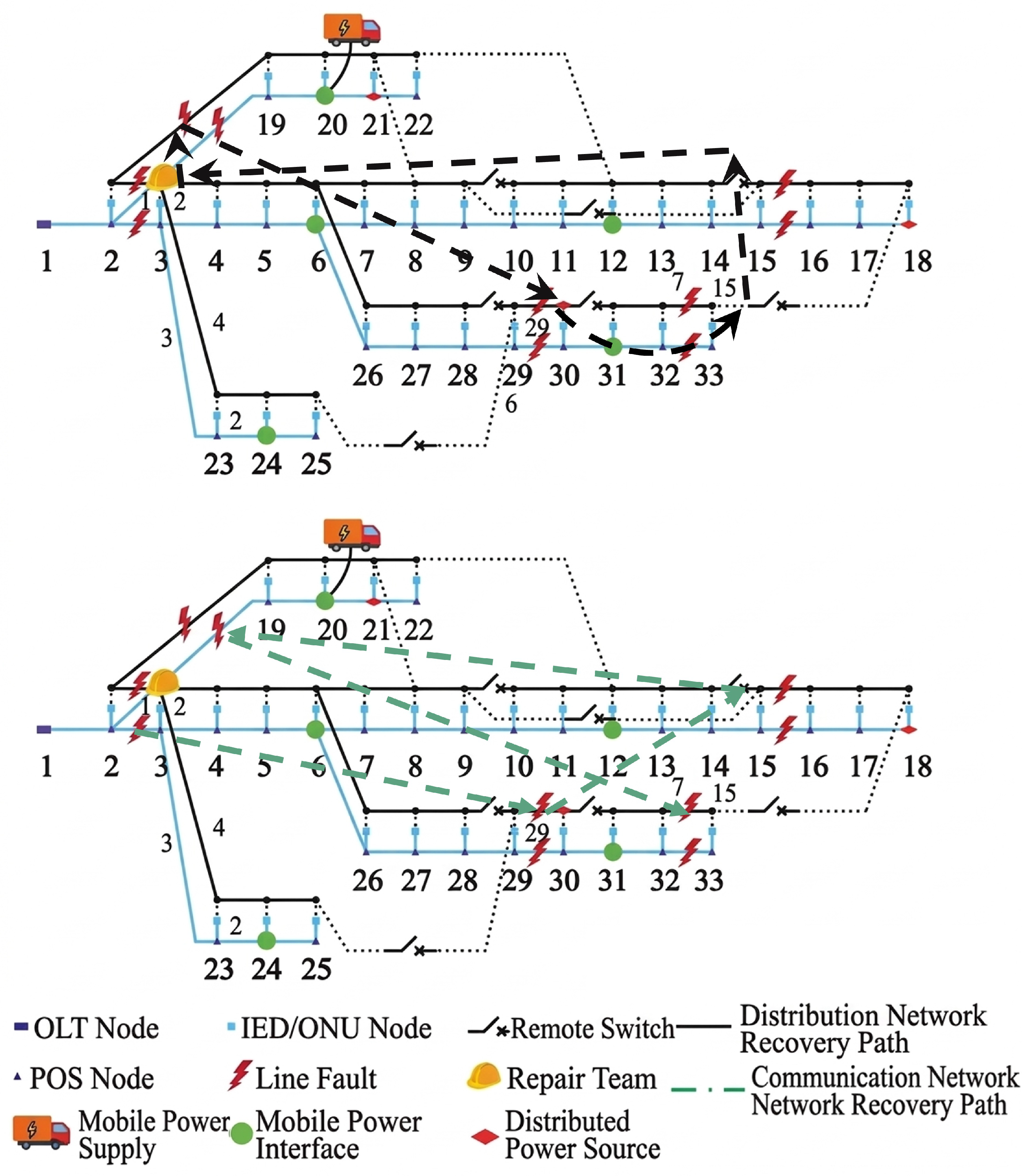
The schematic diagram of the deployment and restoration results for the worst case is illustrated in Figure 3. The pre-disaster deployment locations under the proposed method are summarized as follows. The repair crew for the distribution network is pre-positioned at depot node 2, and the crew for the communication network is pre-positioned at node 2, both near the most failure-prone corridors. The mobile power source is pre-deployed at node 20 to provide rapid coverage of the heavily loaded mid-feeder region.

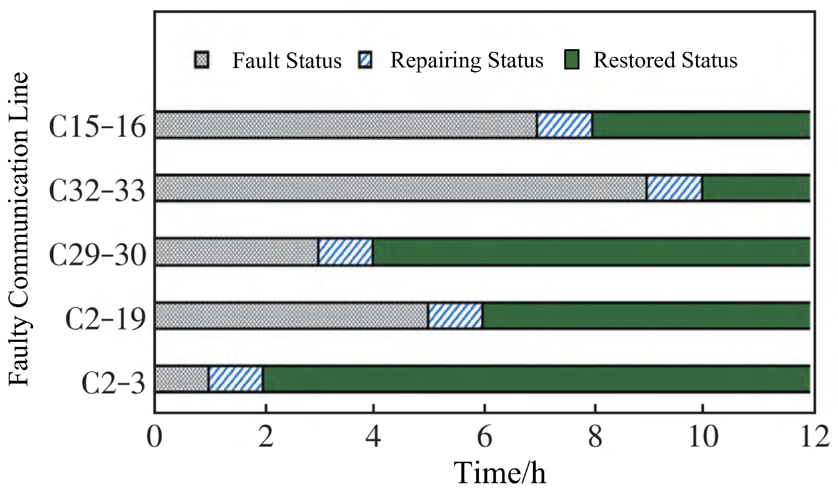
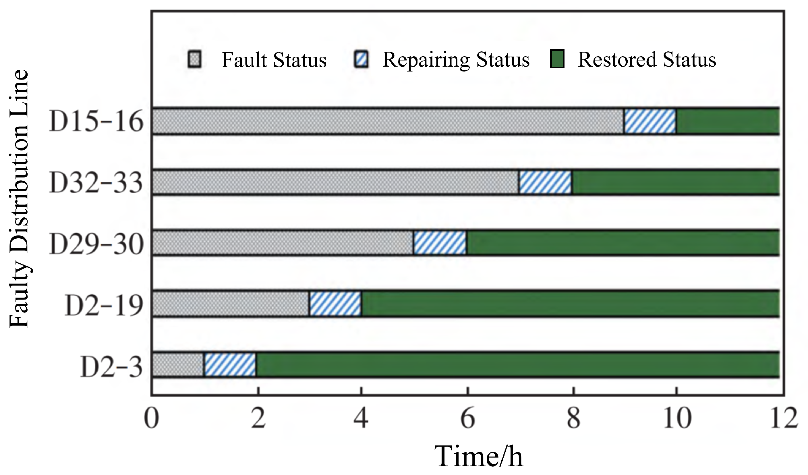
The detailed restoration schedules of the faulted lines are presented in Figure 4 and Figure 5. At hour 1, distribution line D2-3 and communication cable C2-3 are damaged, resulting in the loss of communication between the OLT and all network nodes except nodes 1 and 2. Consequently, all distributed generation (DG) units enter islanded operating mode and can only function independently. Due to the failure of distribution line D2-3, the feeder supplies power only to nodes 1 and 2, leaving a large number of customers without electricity. Repair crews are dispatched to D2-3 and C2-3, respectively, while the mobile power source begins supplying power at node 20 to balance local load demand and provide essential energy support for communication restoration.

At hour 2, D2-3 and C2-3 are repaired. Although some nodes temporarily remain without grid power, the mobile power source sustains electricity supply for critical communication nodes, ensuring partial restoration of communication functions. During this stage, the mobile power source effectively operates as a microgrid controller, maintaining communication services in the disaster-affected area. The priority at this stage is to restore critical distribution and communication lines to enhance load and communication recovery as rapidly as possible.

At hour 3, with D2-3 and C2-3 fully restored, most nodes gradually regain both power supply and communication capability. The repair crews proceed toward distribution line D2-19 and communication cable C29-30, while the mobile power source moves toward node 6. If communication line C2-19 were intact, closing the remote-controlled switches of distribution lines D8-21 or D12-22 (as shown in Figure 3) would fully satisfy the load demand of buses 19, 20, 21, and 22. However, due to the failure of C2-19, the remote-controlled switch of D8-21 remains open because the DG at bus 21 operates in island mode, and the switch of D12-22 remains open since the corresponding control node at bus 22 is de-energized. Meanwhile, through coordinated microgrid dispatch, the mobile power source supports these buses and alleviates power shortages.

At hour 4, D2-19 and C29-30 are under repair, and the mobile power source begins supplying power at node 6. Since the DG at bus 21 remains disconnected from the communication network, it continues operating in island mode, and bus 22 remains de-energized. At hour 5, the two repair crews move toward D29-30 and C15-16, further advancing system restoration.

At hour 6, the mobile power source relocates to node 24, while repair crews conduct restoration of D29-30 and C15-16. Upon completion, they proceed at hour 7 toward D32-33 and C2-19. As shown in Figure 3, buses 16, 17, and 18 are not directly connected to the feeder. Since communication with the DG at bus 18 has been restored, the critical load at bus 16 is preferentially supplied by this DG, which forms a local microgrid to support regional power supply and dynamically coordinates with other microgrids. Although bus 33 can be connected to bus 18 by closing the remote-controlled switch on line D18-33, the limited capacity of the DG prevents it from satisfying all loads at buses 16, 17, 18, and 33 simultaneously.

At hour 8, the mobile power source begins supplying power at node 24. Repair crews restore distribution line D32-33 and communication cable C2-19, and subsequently complete restoration of D15-16 and C32-33 at hour 10. At this point, system load demand is largely satisfied. The loads at buses 16, 17, and 18 are fully restored through the remote-controlled switch on D18-33. Both the power distribution network and communication network return to normal operation, effectively mitigating the large-scale outage caused by the disaster.

5.1.2. Pre-Disaster Resource Deployment Comparative Analysis

To evaluate the effectiveness of the proposed pre-disaster deployment strategy, three resource allocation schemes are compared under a Monte Carlo-based multi-scenario framework comprising 100 randomly generated damage scenarios:

• Proposed method: Pre-disaster resource positions are optimized via the progressive hedging algorithm across all generated scenarios.
• Heuristic strategy: Resources are preferentially allocated to components with the highest damage probability; i.e., those ranked by vulnerability index.
• Random strategy: Resources are randomly assigned to candidate positions without scenario information.

For the heuristic deployment strategy, emergency resources are allocated according to the vulnerability ranking of system components. The distribution repair crew is positioned at node 3, which is adjacent to the high-risk distribution lines D2-3 and D3-4. The communication repair crew is deployed at node 4 near the communication cables with relatively high failure probability. The mobile power source is placed at node 25 to provide backup support to the downstream feeder region with considerable load demand.

For the random deployment strategy, emergency resources are assigned to candidate nodes without considering vulnerability or load distribution. In this study, the distribution repair crew is randomly placed at node 12, the communication repair crew at node 20, and the mobile power source at node 30.

A quantitative comparison of average load shedding and restoration completion time across scenarios is presented in

Table 2. Comparison of pre-disaster deployment strategies.

Strategy	Avg. Load Shedding (kW·h)	Avg. Restoration Time (min)
Proposed	1153.2	500
Heuristic	1731.8	580
Random	2153.2	680

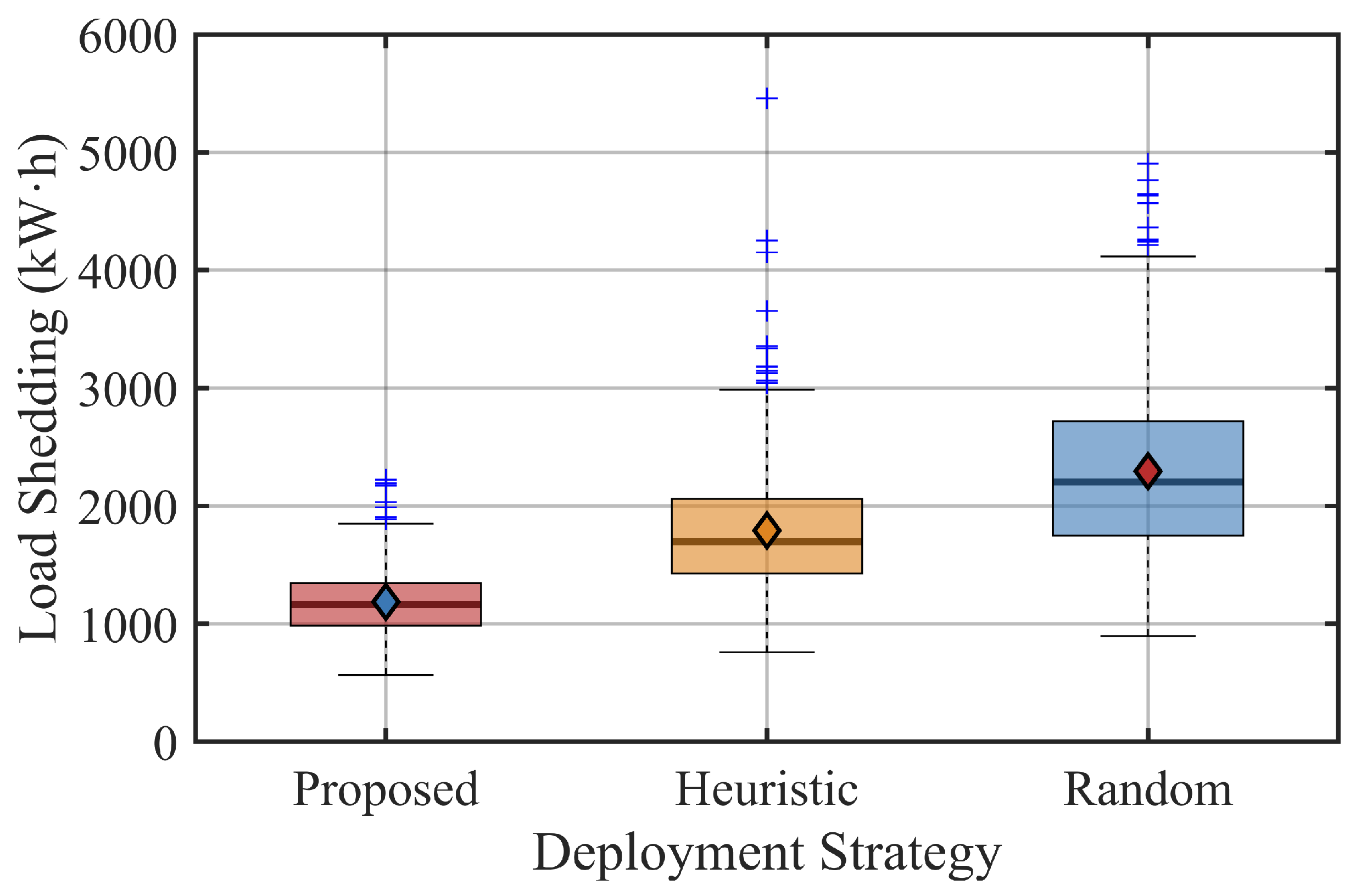
. Figure 6 illustrates the load shedding distributions under the three strategies.

As shown in Table 2 and Figure 6, the proposed deployment strategy achieves the lowest average load shedding and the shortest restoration time among the three compared schemes. Specifically, the average load shedding under the proposed method is 1153.2 kW·h, which is 33.4% lower than that of the heuristic strategy and 46.5% lower than that of the random strategy. In terms of restoration efficiency, the proposed strategy completes system restoration within 540 min, reducing the restoration time by 6.9% compared with the heuristic strategy and by 20.6% compared with the random strategy.These results demonstrate that the proposed pre-disaster deployment strategy can effectively reduce system load loss and accelerate post-disaster recovery. The heuristic strategy performs moderately because allocating resources based on component vulnerability partially reflects the spatial distribution of failure risk. However, it does not account for the coordinated routing and scheduling of restoration resources, which limits its overall effectiveness. In contrast, the random strategy lacks scenario-oriented optimization and therefore results in the largest load shedding and the longest restoration time. Overall, the proposed method significantly improves both restoration efficiency and system resilience by optimizing resource pre-positioning under multiple disaster scenarios.

5.1.3. Post-Disaster Restoration Comparative Analysis

To demonstrate the superiority of the proposed approach, four restoration strategies are compared under the same disaster scenario.

Method 1: Coordinated repair crew and MPS dispatch without considering the communication network [9].

Method 2: Cyber-physical coupled restoration where the communication network influences only remote switching operations but does not affect repair scheduling [14].

Method 3: Cyber-physical restoration with switching coordination but without mobile power sources [16].

Method 4 (proposed): Jointly considers repair crew routing, MPS deployment, and distribution-communication network coordination.

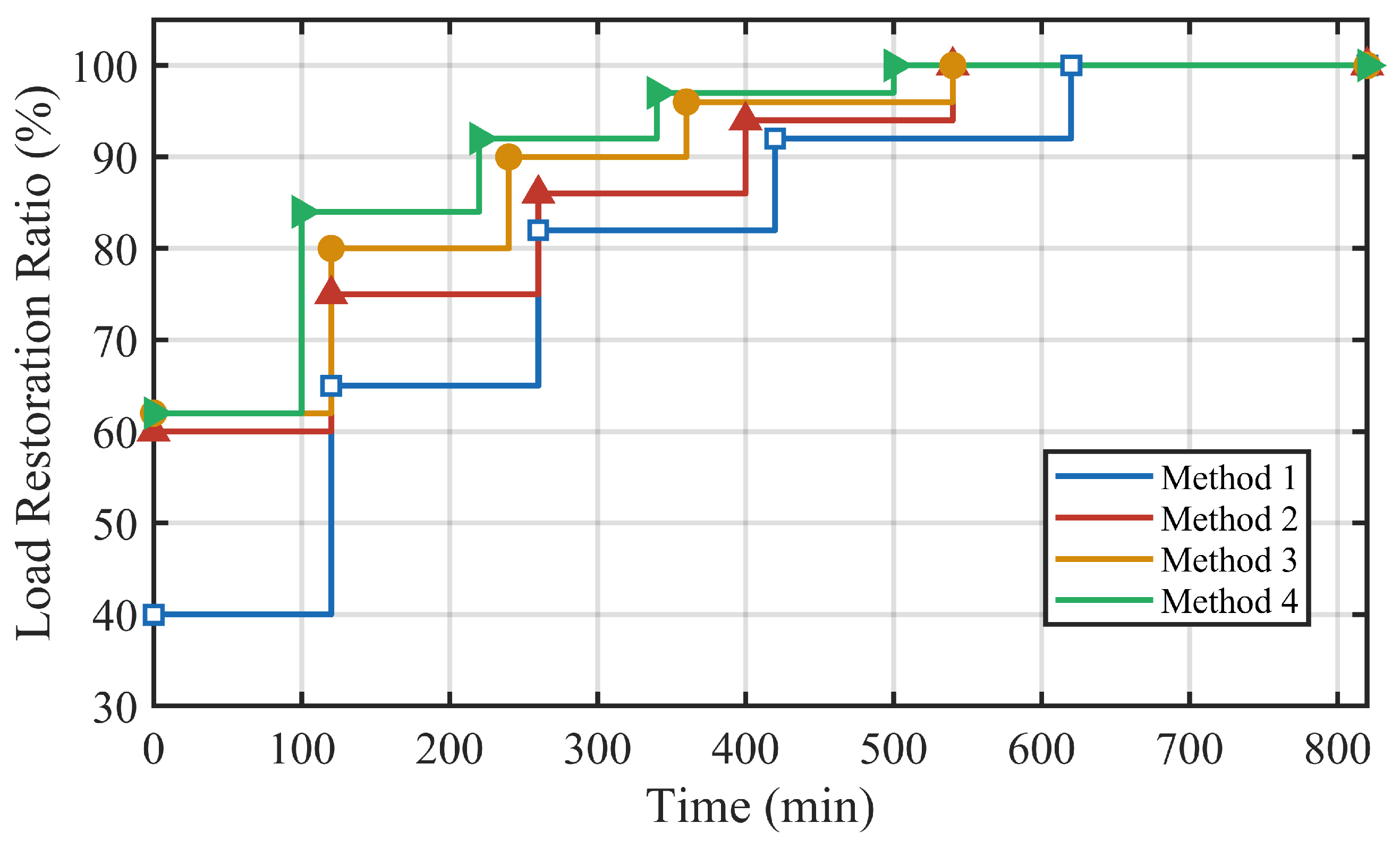
The load restoration ratio of the four strategies under the worst-case scenario is shown in Figure 7. As illustrated in Figure 7, the proposed method outperforms the other three strategies in terms of both restoration speed and overall recovery performance.

The load restoration ratio of the four strategies under the worst-case scenario is illustrated in Figure 7. As shown in the figure, the restoration trajectories of the four methods exhibit noticeable differences in both the restoration speed and the achievable load recovery level.

For Method 1, the absence of communication network support limits the coordination between repair actions and system operation. As a result, the restoration process proceeds relatively slowly. As shown in Figure 7, the restored load ratio is only 40% at the initial stage, and increases to 65% after approximately 2 h. Even after 6 h, the restored load reaches only about 82%, which is significantly lower than the other strategies during the same period. The load restoration ratio gradually increases to around 92% at approximately 7 h, and full restoration is not achieved until about 10 h. This result indicates that the lack of communication-assisted coordination significantly reduces restoration efficiency.

For Method 2, the communication system enables remote switching coordination, which partially improves restoration efficiency. As shown in Figure 7, the restored load ratio reaches approximately 75% within the first 2 h, which is higher than that of Method 1. At around 6 h, the load restoration ratio increases to approximately 86%, and further rises to about 95% at around 7 h. Although the restoration performance is improved compared with Method 1, the absence of communication-assisted repair scheduling still limits the overall restoration speed.

For Method 3, the restoration process benefits from the coordination between the distribution and communication networks. However, the absence of mobile power sources restricts the system’s ability to provide temporary power supply to isolated load areas during the early restoration stage. As a result, the initial load restoration level is higher than that of Method 2 but still increases at a moderate pace. Although the restoration performance continues to improve as faults are gradually repaired, the lack of mobile power support limits the flexibility of the restoration process.

Method 4 simultaneously considers repair crew routing, mobile power source deployment, and the coordinated restoration of the distribution and communication networks. By jointly optimizing repair scheduling, network switching operations, and temporary power supply support, the proposed strategy significantly accelerates the restoration process. As shown in Figure 7, Method 4 achieves the fastest load recovery among the four strategies. A relatively high restoration level is achieved during the early stage, and the load restoration ratio continues to increase steadily as repair operations progress. Eventually, the system approaches full restoration earlier than the other methods.

Overall, the results demonstrate that the proposed coordinated restoration strategy significantly improves both the restoration speed and load recovery level. By integrating repair crew dispatching, mobile power support, and communication–distribution network coordination, the proposed method provides a more efficient and resilient recovery framework under extreme disaster conditions.

Table 3. Quantitative comparison of four restoration methods.

Method	Total Load Loss (kW·h)	Restoration Time (min)
Method 1 (MPS, no comm.)	2283.6	620
Method 2 (comm.→switch only)	1612.3	540
Method 3 (no MPS)	1583.8	540
Method 4 (proposed)	1153.2	500

presents a quantitative comparison of the four restoration strategies in terms of total load loss and restoration time. As shown in the table, Method 4 (the proposed strategy) achieves the best performance among all methods. Specifically, the total load loss is reduced to 1153.2 kW·h, which represents a reduction of 49.5%, 28.5%, and 27.2% compared with Method 1, Method 2, and Method 3, respectively. In addition, the restoration time is shortened to 500 min, which is 120 min earlier than Method 1 and 40 min earlier than both Method 2 and Method 3. These results indicate that the joint optimization of repair crew routing, mobile power source deployment, and distribution–communication network coordination significantly improves restoration efficiency and effectively reduces load loss during the recovery process.

5.2. Sensitivity Analysis

To systematically evaluate the robustness of the proposed model, a multi-dimensional parameter sweep is conducted covering fault severity and mobile power source capacities, as described below.

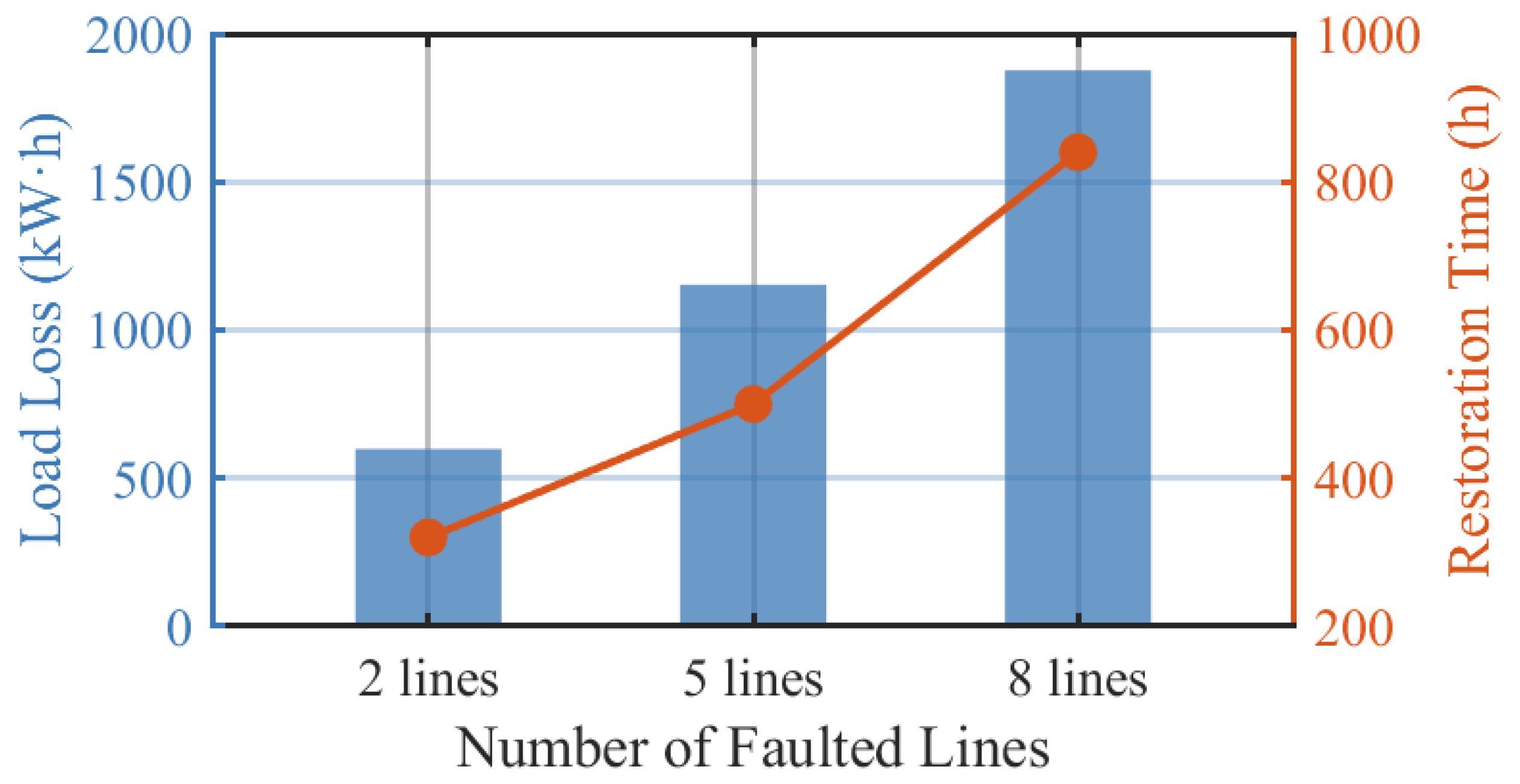
Three fault severity levels are considered: 2, 5, and 8 simultaneously faulted distribution lines (with corresponding communication cables co-located on the same corridors also failing).

Table 4. Impact of fault severity on restoration performance.

Faulted Lines	Load Loss (kW·h)	Restoration Time (min)
2	598.4	320
5	1153.2	500
8	1876.3	840

and Figure 8 present the results.

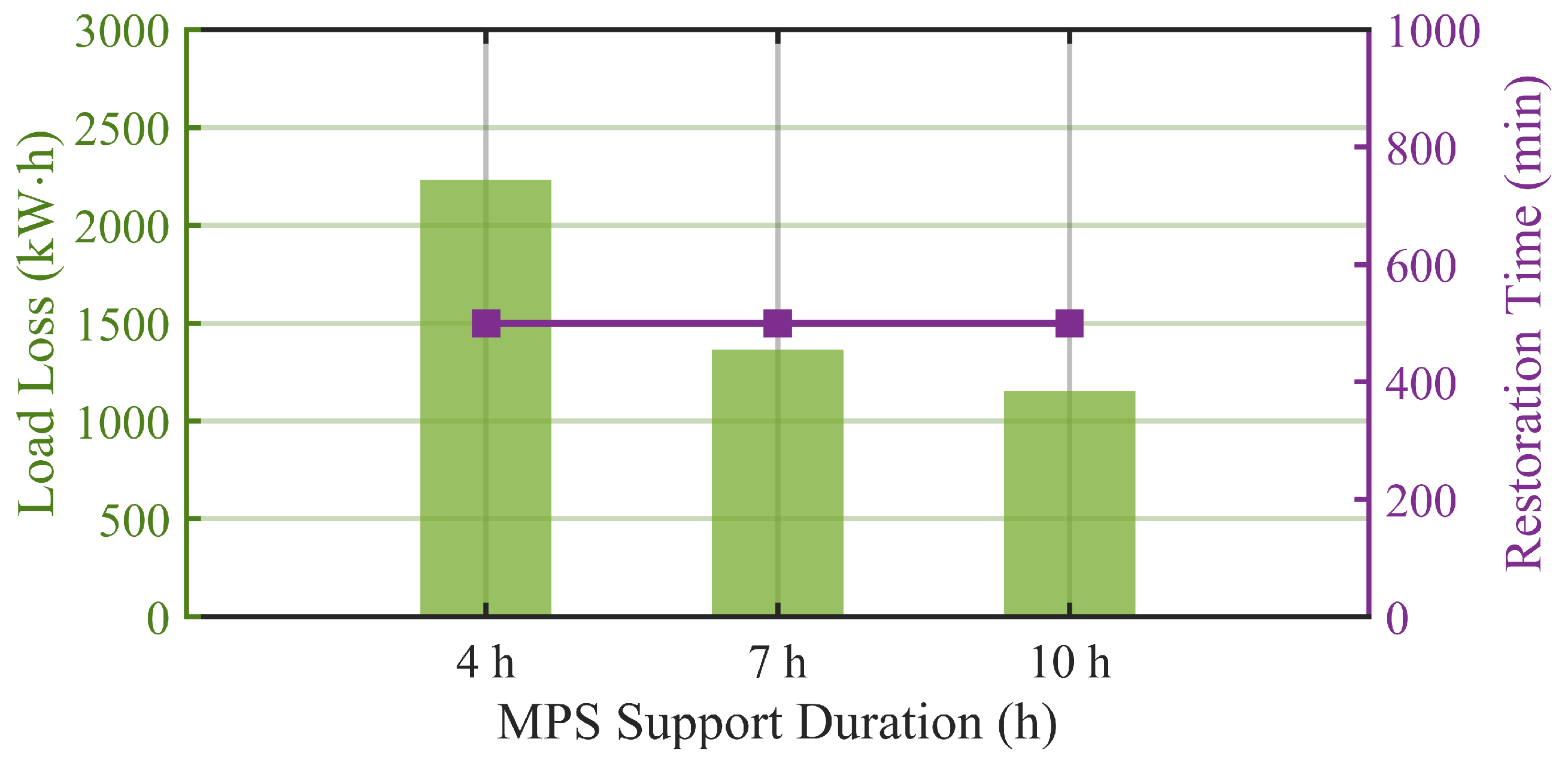
Three mobile power source capacity levels are considered, corresponding to load support durations of 4 h, 7 h, and 10 h. The results are presented in

Table 5. Impact of mobile power source capacities on restoration performance.

MPS Support Duration (h)	Load Loss (kW·h)	Restoration Time (min)
4	2231.6	500
7	1364.7	500
10	1153.2	500

and Figure 9.

As fault severity increases from 2 to 8 damaged lines, load loss grows nonlinearly from 598.4 to 1876.3 kW·h, representing an overall increase of approximately 213.5%. Restoration time likewise extends from 320 to 840 min, a growth of 162.5%. Notably, the marginal impact accelerates with fault scale: escalating from 2 to 5 faulted lines raises load loss by 92.7% (from 598.4 to 1153.2 kW·h), whereas a further increase from 5 to 8 lines adds another 62.7% (reaching 1876.3 kW·h), accompanied by a disproportionate jump in restoration time from 500 to 840 min (+68.0%). This nonlinear growth reflects the compounding effect of simultaneous communication and distribution failures: each additional co-located fault further isolates both power and communication infrastructure, reducing the effectiveness of MPS dispatch and remote switching. Even under the most severe scenario (8 faulted lines), the proposed method maintains systematic restoration progress, validating its scalability under large-scale contingencies.

Regarding MPS capacity, extending the support duration from 4 h to 10 h reduces load loss from 2231.6 to 1153.2 kW·h, a reduction of approximately 48.3%. The improvement is most pronounced in the first capacity increment: increasing support duration from 4 h to 7 h alone cuts load loss by 38.8% (from 2231.6 to 1364.7 kW·h), while the subsequent increase from 7 h to 10 h yields a more moderate additional reduction of 15.5%. In contrast, restoration time remains stable at 500 min across all three capacity scenarios, indicating that the routing and scheduling logic can fully exploit additional energy within the same time horizon. These results highlight the diminishing-returns nature of MPS capacity expansion: substantial initial gains can be achieved with moderate capacity increases, while further enlargement provides incrementally smaller benefits. Consequently, the 7 h configuration offers a favorable cost-effectiveness trade-off, capturing the majority of available load-loss reduction without requiring maximum-capacity deployment.

6. Conclusions

This study proposes a unified framework for pre-disaster deployment and post-disaster restoration of coupled distribution and communication networks under extreme disaster conditions. Case studies conducted on a modified IEEE 33-bus cyber–physical distribution system validate the effectiveness of the proposed method under coupled failure scenarios. The results show that the proposed coordinated planning strategy reduces load loss by 33.4% and 46.5% compared with the heuristic deployment strategy and the random deployment strategy, respectively. In addition, the proposed coordinated restoration strategy is capable of restoring approximately 50% of critical loads within the first three hours after the disaster, which is of great practical significance for maintaining the operation of essential infrastructures such as hospitals, emergency shelters, and communication hubs during the early stage of disaster recovery.

Despite the promising results, several directions remain for future research. First, future work may consider integrating emerging emergency communication technologies, such as unmanned aerial vehicle (UAV)-based communication stations and emergency communication vehicles, to further improve adaptability in complex disaster environments. Second, the influence of transportation network disruptions on repair crew mobility could be explicitly modeled to enhance practical applicability. Finally, to address computational challenges in large-scale systems, advanced solution techniques such as decomposition algorithms or machine learning-assisted optimization methods may be explored to improve computational efficiency while maintaining solution quality.