Unmasking Biases and Reliability Concerns in Convolutional Neural Networks Analysis of Cancer Pathology Images

Abstract

Convolutional Neural Networks have shown promising effectiveness in identifying different types of cancer from radiographs. However, the opaque nature of CNNs makes it difficult to fully understand the way they operate, limiting their assessment to empirical evaluation. Here we study the soundness of the standard practices by which CNNs are evaluated for the purpose of cancer pathology. Thirteen highly used cancer benchmark datasets were analyzed, using four common CNN architectures and different types of cancer, such as melanoma, carcinoma, colorectal cancer, and lung cancer. We compared the accuracy of each model with that of datasets made of cropped segments from the background of the original images that do not contain clinically relevant content. Because the rendered datasets contain no clinical information, the null hypothesis is that the CNNs should provide mere chance-based accuracy when classifying these datasets. The results show that the CNN models provided high accuracy when using the cropped segments, sometimes as high as 93%, even though they lacked biomedical information. These results show that some CNN architectures are more sensitive to bias than others. The analysis shows that the common practices of machine learning evaluation might lead to unreliable results when applied to cancer pathology. These biases are very difficult to identify, and might mislead researchers as they use available benchmark datasets to test the efficacy of CNN methods.

1. Introduction

Pathology benchmark datasets play a critical role in advancing automatic diagnostic systems through the use of deep learning and other machine learning models [1,2,3,4,5,6,7,8,9,10]. These biomedical images can be used to train machine learning systems to identify cancer through different types of imaging modalities, such as X-rays [11], Magnetic Resonance Imaging (MRI) [12,13], Positron Emission Tomography (PET) [14], Computed Tomography (CT) [15,16], Optical Coherence Tomography (OCT) [17], ultrasound [18], and endoscopy [19].

Artificial Intelligence (AI), and specifically deep neural networks, have been advancing rapidly, with a significant impact on various scientific domains. Convolutional neural networks [20,21] have become the dominant approach to image recognition and analysis tasks. Their ability to learn features directly from the data has led to significant advancements in various fields related to computer vision, including automated image-based pathology [22].

However, despite their numerous strengths, CNNs also have some notable drawbacks. Unlike feature-engineered models that are structured to make predictions from hand-crafted features, CNNs’ extraction of features is fully automated. This fully integrated learning ability is useful in domains such as biomedical imaging, which involve complex data-driven feature selection [23,24,25].

However, because CNNs are practically not interpretable, the common means of performance evaluation is through empirical experiments. These evaluation practices are commonly used in the field of machine learning, and include performance indicators such as the classification accuracy, sensitivity, specificity, F-1, confusion matrix, and more.

However, the widespread development and adoption of CNNs in fields such as healthcare requires strict scrutiny beyond mere performance metrics. Therefore, the experimental design used in the field of machine learning might not be fully suitable for cancer pathology.

CNN architectures can exhibit biases that may lead to inaccurate clinical and research results, and can mislead even experienced researchers [26,27,28]. For instance, unnoticeable changes in factors such as the position of the scanner or patient, the temperature of the charged-coupled device sensor used for the collection of images, and even the different technicians who acquire the data can lead to certain differences that are difficult to detect with the naked eye but can have a significant influence on CNNs [28].

In this study we examine the presence and impact of dataset bias on CNN analysis applied to cancer pathology. This is achieved by testing the ability of CNN models to identify cancer based purely on extracted background regions of original cancer pathology images that do not contain medically relevant information. The ability of a CNN to identify cancer from these background sections indicates that their performance demonstrated might be driven by bias rather than a true ability to identify cancer.

This study uses 13 well-known cancer pathology benchmark datasets that have already been cited thousands of times in the cancer pathology literature. The study examines these datasets in combination with some of the most common CNN architectures to profile the differences between these architectures in the context of dataset bias.

The analysis reveals a concerning trend, which further underscores the significance of understanding what CNN models are learning in biomedical image analysis. The classification accuracies of CNNs trained on cropped background images are noticeably higher than mere chance accuracy and are close to the classification accuracy of the trained original images in some cases.

These findings show that traditional machine learning performance evaluation practices might not be ideal for the field of cancer pathology. Testing CNNs using some of the common benchmark datasets might lead to biased results that do not reflect the true ability of CNNs to identify cancer. These findings should be used as a recommendation to conduct empirical evaluations of CNN with caution.

Related Work

Dataset bias has been discussed in the context of machine learning before deep neural networks were introduced [29]. Unbalanced datasets have been a known source of dataset bias, and several approaches have been proposed to handle unbalanced data [30]. Other biases, driven by the annotation of the dataset or the dataset design, were also noted before CNNs became common [29,31].

As CNNs became the primary solution to image analysis, other biases driven by the method of acquisition of the images were reported [27,32,33]. These biases showed that CNNs are sensitive to information that cannot be sensed by the unaided human eye, yet allow CNNs to provide good classification accuracy.

Biases were also observed in biomedical images [26,27,28,34]. Studies have shown that CNN models often learn to exploit superficial correlations or background artifacts in training data, learning features and patterns that are highly predictive but not directly associated with the underlying disease pathology [28,35,36]. For example, CNNs rely on hospital-origin metadata tags and radiographic positioning rather than lung pathology, as shown when trained on chest X-rays [36].

This phenomenon, known as shortcut learning, refers to the situation when machine learning models do not learn from meaningful features to make decisions, but instead focus on easy-to-learn features that can lead to good performance on training datasets but poor generalization on unseen data. However, this has not been profiled in the context of cancer pathology via a thorough analysis of different datasets and CNN architectures.

2. Methods

We performed a series of experiments on thirteen highly used biomedical image datasets. The experiments focused on the automatic classification of radiographs using four commonly used CNN models: ResNet50 [37], DenseNet121 [38], Inception V3 [39], and VGG16 [40]. These architectures were selected because they are among the most commonly used CNN architectures. While they are used extensively in all domains, these architectures are widely used for the purpose of cancer pathology [41,42,43,44].

2.1. Experimental Design

In many cases, a radiograph has some clinically relevant parts, while other parts of the radiograph do not contain information that can allow for diagnosis. The presence of some regions that do not contain clinical information allow for the reliability of CNNs to be tested when applied to cancer pathology. If the performance evaluation is undertaken using only the parts of the radiographs that are not clinically relevant, it can provide an indication of bias in the analysis.

Naturally, parts of the radiograph that do not contain parts of the body or other relevant medical information are not expected to allow for the diagnosis of cancer. Therefore, if the standard performance evaluation provides satisfactory results when using only medically irrelevant parts of the radiographs, that can indicate that the evaluation might be unsound. Such deceiving performance evaluation can be driven by biases that are very difficult to identify.

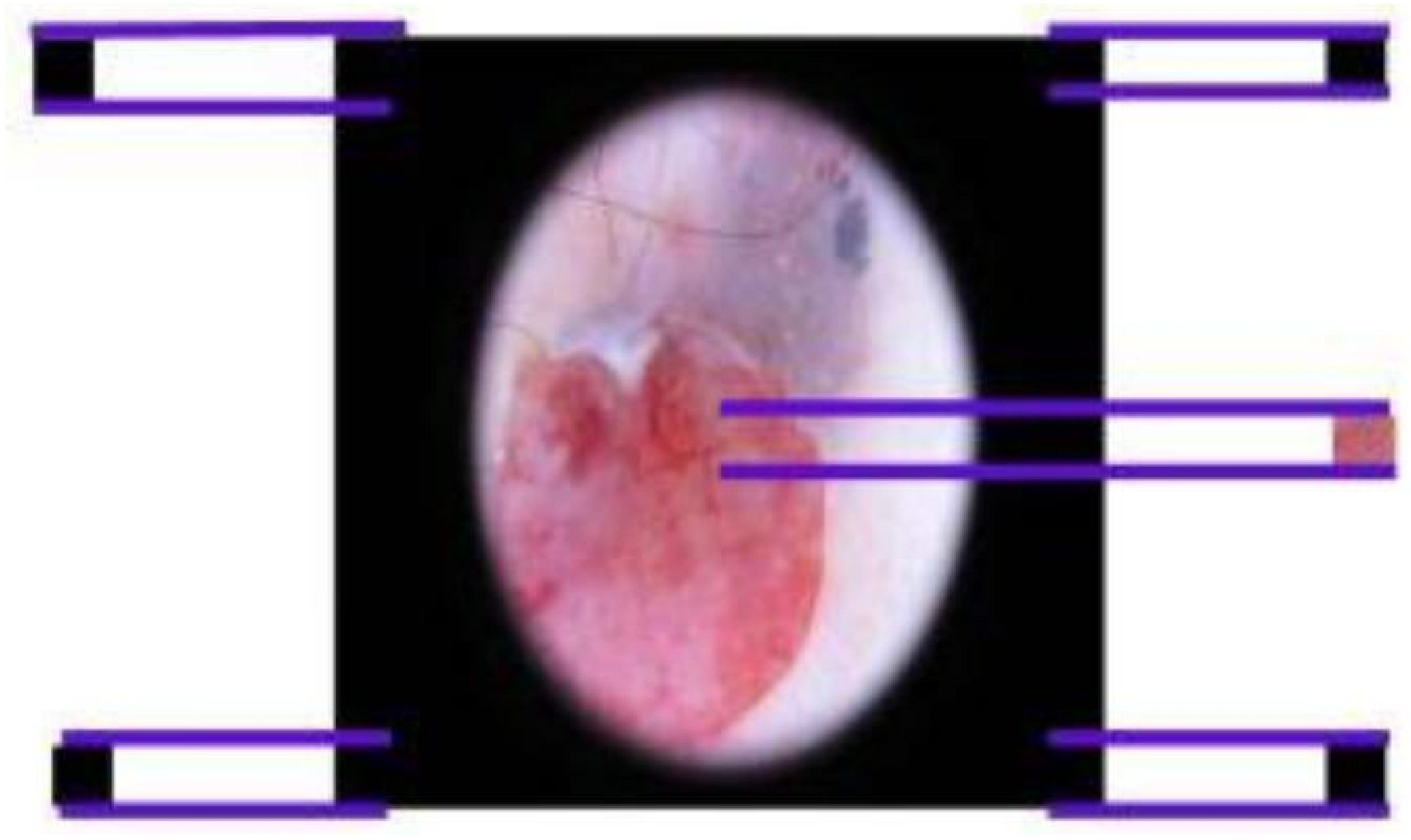
To test for such biases, we compare the performance achieved with the original images to the performance observed with small sub-images that do not contain medical information. These cropped images are 20 × 20 pixel sub-images [27,33] from five different parts of each original image: upper-left, upper-right, center, bottom-left, and bottom-right. That is, from each dataset, we create five new datasets with the same number of classes and the same number of images. Instead of the original images, the dataset contains small images separated from the non-medical parts of the original images. In this study, the cropping of the images was achieved with the Python Imaging Library (PIL) 11.2.1, which is a common library for basic image processing [45]. All cropping was done in a fully automatic manner to avoid any possible human bias.

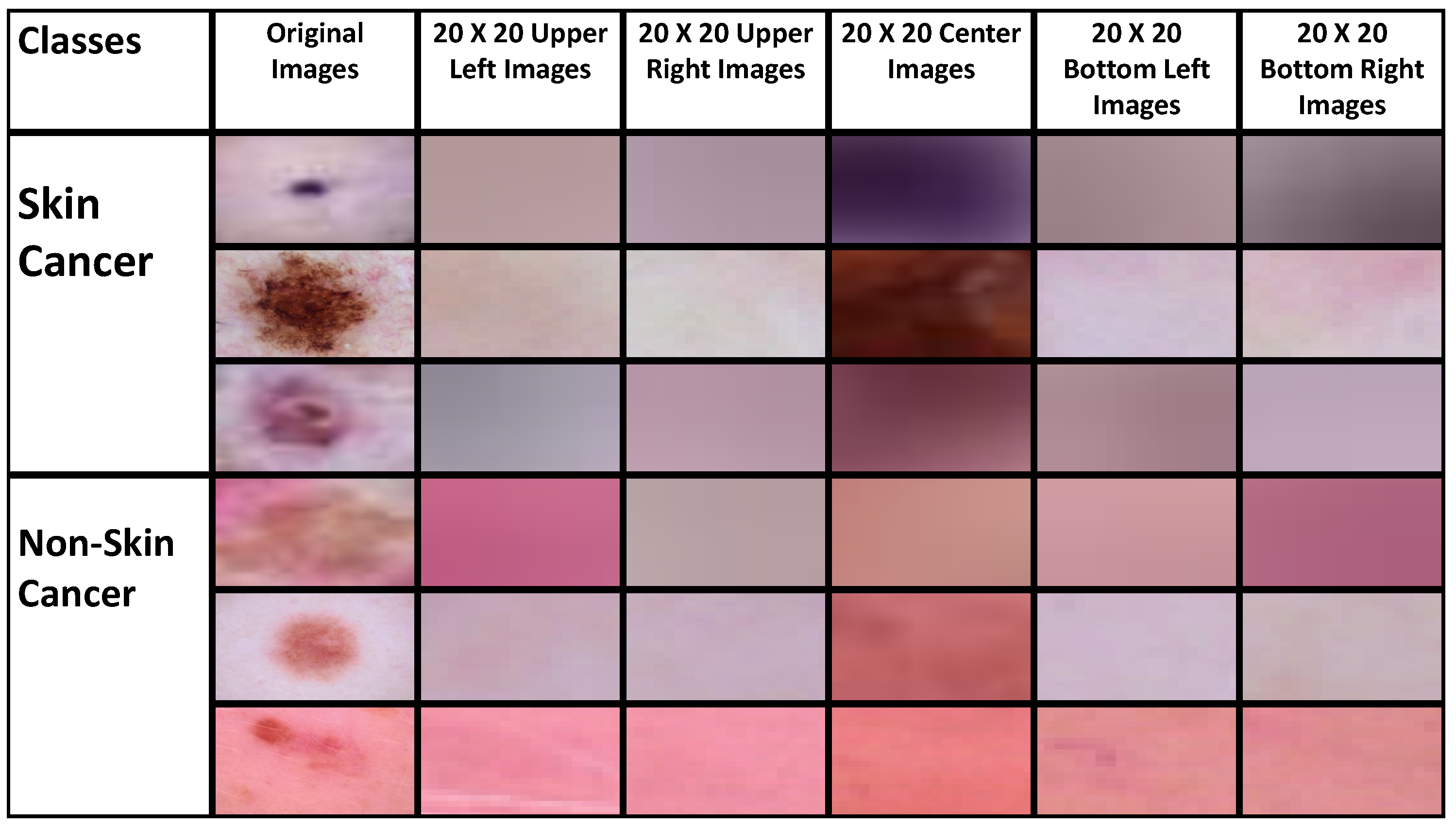
Figure 1 shows how and where each of the five 20 × 20 sub-images were cropped from the original image. Figure 2 shows examples of the original image, with corresponding cropped five sections that depict both benign and malignant tissues, forming the basis for two classes. While the full original image allows for diagnostics, the five new datasets created from it are too small to analyze the structure of the tissue, and are not sufficiently informative to provide a reliable diagnostics.

To test the ability of the CNNs to classify the images, we first split the original dataset into training and test/validation datasets using the standard 80/10/10 practice. The dataset is then tested by using the neural network architecture to evaluate the ability of the neural network to identify between positive and negative cases. The same process is repeated with each of the five datasets generated from the original dataset. The ability of the neural network to identify cancer from each of these datasets is compared to the performance when using the original dataset with the full images.

2.2. Model Architecture

Unless stated otherwise, the training was performed with the commonly used practice of transfer learning using pre-trained ImageNet weights. The input image resolution is model-dependent, and the images were adjusted to the model input. A standardized input resolution of 224 × 224 was used for ResNet-50, DenseNet-121, and VGG16, while 299 × 299 was used for Inception V3 in line with the training convention of each model.

Modifications were made by replacing the final classification layer of each model with a fully connected layer, producing two logit models to support a two-class classification task (cancer present or cancer absent). A softmax layer was applied as the final layer to produce a probability distribution that facilitates decision-making.

All four models were trained using the standard Adam optimizer [46]. A constant learning rate of 0.0001 was used for each model across all experiments. This can help to achieve better stability and convergence, further improving generalization accuracy [47]. Unless stated otherwise, the training was conducted over five epochs, which is sufficient for convergence and the use of transfer learning models. Furthermore, a batch size of 32 training samples was used in one iteration during training, balancing the models’ performance between computational efficiency and quality of learning.

As discussed above, each dataset provided five additional datasets, such that each new dataset was made from only cropped images containing a certain part of the original images. For consistency, the exact same practices were used for each of these new datasets, including the cropping, resolution, and architecture parameter settings as described above. The same parameters were also used for testing the original images.

The computing was carried out using the Beocat computing facility [48]. Beocat is a powerful cluster with over 11,000 CPU cores. To train the CNNs, we used GPUs. Beocat has 90 GPU-enabled nodes that host 170 GPUs, with models ranging from the simple GeForce GTX 1080 Ti to the advanced nVidia L40S. This cluster provides powerful computing that can enable a large number of CNN experiments.

2.3. Biomedical Images Datasets

We obtained thirteen publicly available benchmark biomedical image datasets frequently used for developing and testing CNN methodology for cancer diagnosis. In these experiments, we use these datasets to evaluate the performance of CNN architectures on cancerous versus noncancerous tissues.

The datasets were selected based on their prevalence as benchmarks for developing and testing CNN-based methods for cancer pathology. The datasets that were chosen were all highly cited in the literature, and therefore an analysis of these datasets is required to ensure that they provide a sound platform for the development and testing of reliable CNNs.

These datasets also represent a diversity of types of cancers, modalities, magnifications, and more.

Table 1. The description, class modification, and distribution of samples from the MedMNIST Dataset.

Cancer MedMNIST Dataset
Dataset	Data Modality	Initial Class	Modified Binary Class	Total Samples	Cancer Present Samples	Cancer Absent Samples
PathMNIST	Histopatology	Multi-Class (9)	1. Cancer-Associated Stroma; 2. Colorectal Adenocarcinoma Epithelium = Cancer Present; 3. Adipose Tissue; 4. Background; 5. Debris; 6. Lymphocytes; 7. Mucus; 8. Smooth Muscle and Normal Colon Mucosa = Cancer Absent	107,180	95,435	11,745
DermaMNIST	Dermatoscope	Multi-Class (7)	1. Melanoma; 2. Basal cell carcinoma = Cancer Present; 3. Melanocytic nevi; 4. Benign keratosis-like lesions; 5. Dermatofibroma; 6. Vascular lesions; 7. Actinic keratoses = Cancer Absent	10,015	656	9359
BreastMNIST	Breast Ultrasound	Multi-Class (3)	1. Malignant = Cancer Present; 2. Normal; 3. Benign = Cancer Absent	780	570	210
NoduleMNIST3D	Chest CT	Binary-Class (2)	1. Malignant = Cancer Present; 2. Benign = Cancer Absent	1633	401	1232

shows the different types of cancers included in the experiments, including colorectal tissues, lung tumors, and skin and breast cancer. Modalities include microscopy Hematoxylin and Eosin (H&E) such as in BreakHis, as well as Computed Tomography (CT), X-ray, and ultrasound, as included in the MedMNIST datasets, or the digital camera dermoscopic images included in the ISIC datasets. These cover a broad range of modalities, which are the common modalities used for cancer pathology.

2.4. MedMNIST Datasets

The MedMNIST+ dataset [49] is a larger version of the MedMNIST dataset in terms of image resolution. This improves on the 28 × 28 and 28 × 28 × 28 of the MedMNIST dataset [49,50]. MedMNIST is a standardized collection of eighteen biomedical image datasets for classification with various settings, diversifying the evaluation across pixel size, modalities, and classification tasks [49].

Four datasets from MedMNIST+ were used. These are pathological images suitable for the classification of positive or negative cancer cases. They include the PathMNIST [51], DermaMNIST [52], BreastMNIST [53], and NoudleMNIST [54] datasets. Table 1 shows the structure of these datasets and their respective modification into a binary class. These datasets can be publicly accessed https://zenodo.org/records/10519652 (accessed on 9 March 2026).

2.5. BreakHis Datasets

BreakHis, the Breast Cancer Histopathological Image Classification, is publicly available at https://www.kaggle.com/datasets/ambarish/breakhis (accessed on 9 March 2026). It is a breast cancer histopathology dataset widely used for machine learning research, specifically for classifying images of breast cancer tissues. These histopathology images were collected from 82 patients, containing 7909 image samples [55]. The BreakHis dataset contains different magnification levels: $40\times$, $100\times$, $200\times$, and $400\times$. Each magnification level consists of eight classes, which we modified to suit a binary classification task as described in

Table 2. The Description, class modification, and distribution of samples of the BreakHis Dataset. Figures assigned to each class are as follows: Adenosis = 1; Fibroadenoma = 2; Phyllodes tumor = 3; Tubular adenoma = 4; Ducta carcinoma = 5; Lobular carcinoma = 6; Mucinous carcinoma = 7; and Papillary carcinoma = 8.

BreakHis Dataset
Magnification	Modality	Initial Class	Modified Binary Class	Total Samples	Cancer Present Samples	Cancer Absent Samples
$40\times$	Microscopy Histopathology	Multi-Class (8)	1 to 4 = Cancer Absent/ 5 to 8 = Cancer Present	1995	1370	652
$100\times$				2081	1437	644
$200\times$				2013	1390	623
$400\times$				1820	1232	588

.

2.6. International Skin Imaging Collaboration Datasets

The International Skin Imaging Collaboration (ISIC) is a benchmark dataset associated with a yearly competition for machine learning experts. It consists of a yearly release of dermatoscopic images from 2016 to 2020. This provide standardization for skin imaging, creating an open-access repository of biomedical images. We obtained four datasets, ISIC-2016 [56], ISIC-2017 [57], ISIC-2018 [52,57], and ISIC-2019 [52,57,58], for evaluation, as shown in

Table 3. The description, class modification, and distribution of samples of the ISIC dataset.

The ISIC (2016–2019) Dataset
Dataset	Data Modality	Initial Class	Modified Binary Class	Total Samples	Cancer Present Samples	Cancer Absent Samples
ISIC-2016	Dermatoscope	Binary Class	1. Melanoma = Cancer Present; 2. Benign = Cancer Absent	1279	248	1031
ISIC-2017	Dermatoscope	Multi-Class (3)	1. Melanoma = Cancer Present; 2. Seborrheic_keratosis; 3. Nevus = Cancer Absent	11,527	3736	7790
ISIC-2018	Dermatoscope	Multi-Class (7)	1. Melanoma; 2. Basal cell carcinoma = Cancer Present; 3. Melanocytic nevi; 4. Benign keratosis-like lesions; 5. Dermatofibroma; 6. Vascular lesions; 7. Actinic keratoses = Cancer Absent	10,015	7007	1003
ISIC-2019	Dermatoscope	Multi-Class (8)	1. Malanoma; 2. Besal Cell Carcinoma; 3. Antinic Keratosis; 4. Squamous Cell Carcinoma = Cancer Present; 5. Melanocytic Nevus; 6. Benign Keratosis; 7. Dermotafibroma; 8. Vascular Lesion = Cancer Absent	780	546	78

. These datasets are publicly available at https://challenge.isic-archive.com/ (accessed on 9 March 2026).

2.7. Breast Histopathology Images for Invasive Ductal Carcinoma (IDC) Dataset

The Breast Histopathology Image (IDC) [59] dataset is a benchmark for Invasive Ductal Carcinoma (IDC) detection, specifically designed to classify breast histopathological images as either cancerous (IDC-positive) or non-cancerous (IDC-negative), as shown in

Table 4. Distribution of samples of the Breast Histopathology Image (IDC) Dataset.

Breast Histopathology Image (IDC) Dataset
Dataset	Modality	Initial Class	Modified Binary Class	Total Samples	Cancer Present Samples	Cancer Absent Samples
Breast Histopathology Image (IDC)	Microscopy Histopathology	Binary	IDC-Nagative = Cancer Absent/IDC-Positive = Cancer Present	277,524	78,786	198,738

. The dataset comprises 162 whole-slide images (WSIs) obtained from breast cancer patients, totaling 277,524 images [60]. The dataset is publicly available at https://www.kaggle.com/datasets/paultimothymooney/breast-histopathology-images (accessed on 9 March 2026).

3. Results

3.1. CNNs and MedMNIST+ Datasets

The experiments evaluated the four CNN architectures (ResNet50, DenseNet121, InceptionV3, and VGG16) across four MedMNIST+ datasets. Each MedMNIST+ dataset represents a different type of cancer and imaging modality.

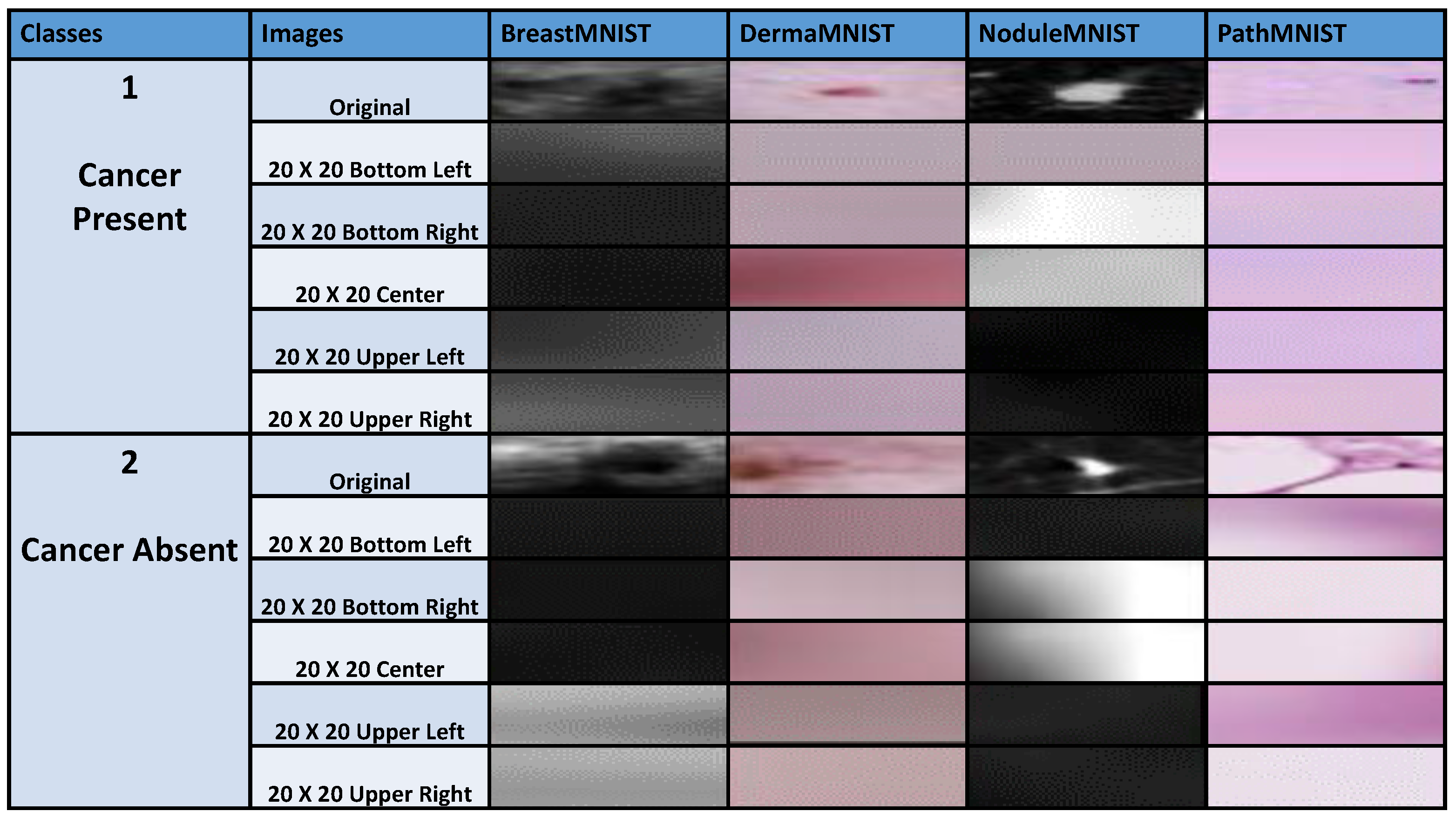
The cropped-image datasets consisted of 20 × 20 pixel extractions from five different sections of the original images (bottom-left, bottom-right, center, upper-left, and upper-right). Due to the differences in lesion size, shape, and location, they often include only background or imaging artifacts, as shown in Figure 3.

3.1.1. BreastMNIST (Ultrasound Scan Imaging)

The BreastMNIST [53] dataset contains two classes: benign and malignant breast tumors. The images are in grayscale echotextures consisting of tissue layers, shadow artifacts, and boundaries. Figure 3 shows sample images, comparing the original and the 20 × 20 cropped-image datasets. Each cropped-image dataset consists of black or gray background images. These background images do not contain tumor structures that would be visible to an expert radiologist to allow for meaningful diagnostics. We do not expect deep neural networks to identify positive and negative cases from these cropped images.

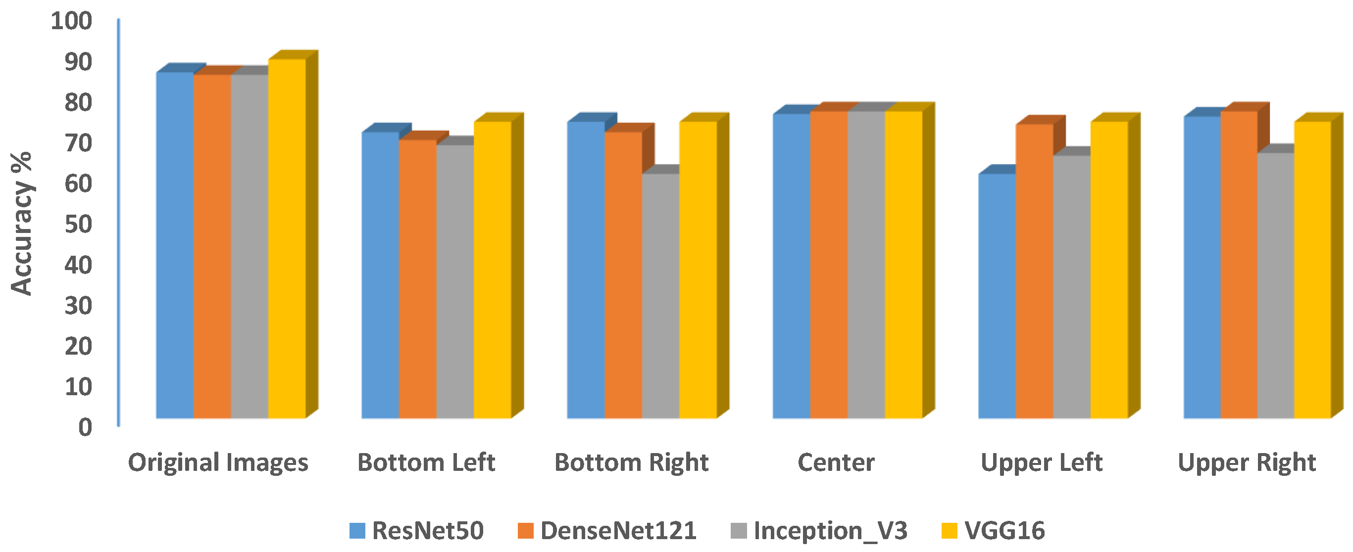
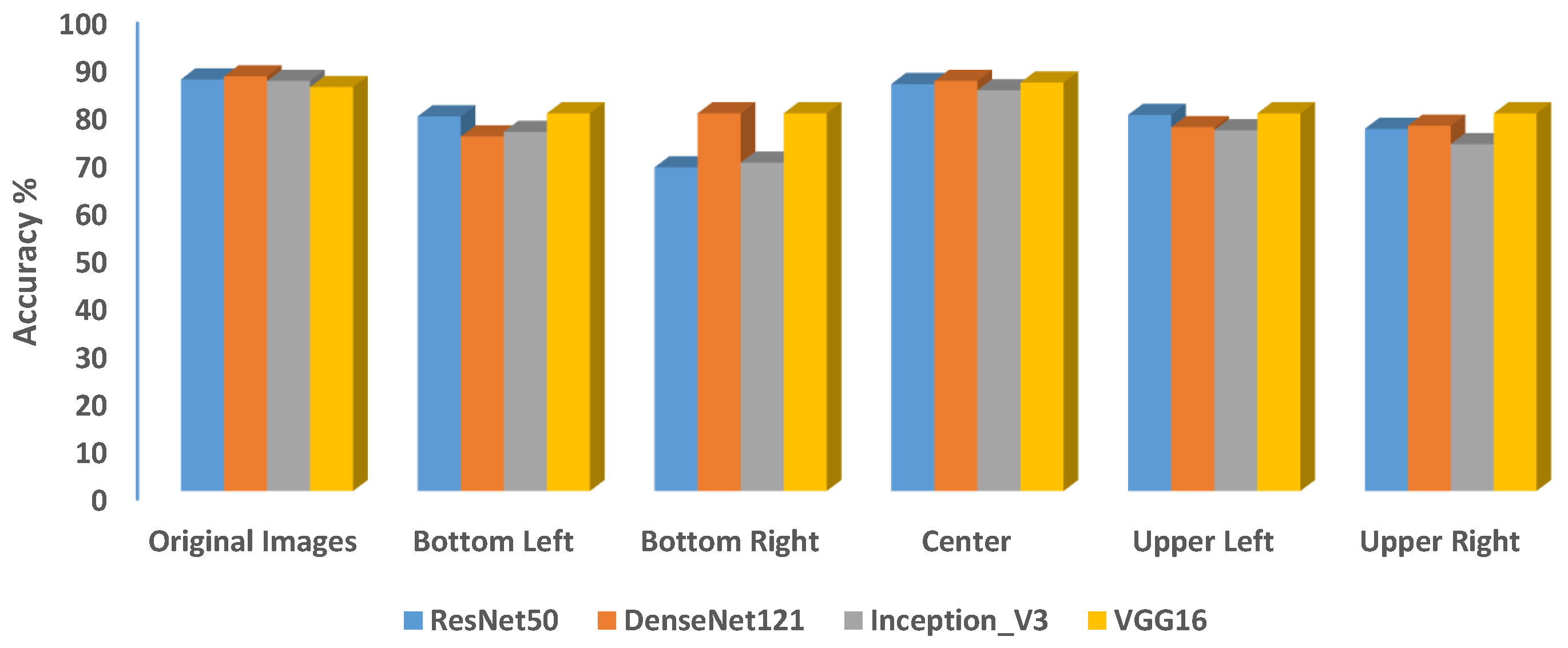
The results from the original images show that CNN architectures can achieve a classification accuracy as high as ∼88.46%. To test for bias, we also experimented on the 20 × 20 pixel image datasets. The results revealed that all CNN models can classify the cropped images with an accuracy well above the mere chance of $50\%$. This performance for a binary classification is not expected, because the cropped images often exclude the tumor region. For example, Figure 4 shows that CNNs can identify cancerous and noncancerous tumors from background images with an accuracy as high as ∼75.64%. That shows that cancer can be identified with an accuracy better than mere chance even when no clinically relevant information is included in the data. Interestingly, VGG16 achieved a consistent performance of ∼73.08% across all cropped-image datasets except the center images.

Table 5. Accuracy, precision, recall, and F-1 results of the analysis of the balanced BreastMNIST.

Model	Sub Dataset	Accuracy	Recall	F1	Precision
DENSENET121	Bottom Left	85.8372	85.5634	81.9552	78.7535
DENSENET121	Bottom Right	62.8590	4.4366	7.4707	28.3412
DENSENET121	Center	62.7399	3.9437	6.8230	35.0489
DENSENET121	Original Images	61.2442	6.5141	10.0572	64.2105
DENSENET121	Upper Left	62.9782	4.6479	7.9069	57.9132
DENSENET121	Upper Right	62.8855	4.7887	7.9559	42.9699
INCEPTION_V3	Bottom Left	84.8312	84.7887	80.8230	77.6369
INCEPTION_V3	Bottom Right	62.6208	2.8169	4.5410	41.0638
INCEPTION_V3	Center	62.7796	2.6761	4.5365	24.9397
INCEPTION_V3	Original Images	62.2766	2.3592	4.1722	19.4480
INCEPTION_V3	Upper Left	62.7929	2.5000	4.2595	29.0031
INCEPTION_V3	Upper Right	62.7929	2.6761	4.5215	25.6140
RESNET50	Bottom Left	85.1621	83.2042	80.8063	78.8106
RESNET50	Bottom Right	63.0443	6.9014	11.4470	58.2067
RESNET50	Center	63.0841	5.8451	9.9479	44.7500
RESNET50	Original Images	61.7737	1.6197	2.8298	13.2013
RESNET50	Upper Left	63.6929	8.2042	13.4575	57.7125
RESNET50	Upper Right	63.6664	7.9930	13.1650	68.3775
VGG16	Bottom Left	82.9385	82.4296	78.4074	74.9589
VGG16	Bottom Right	63.0311	7.9930	11.7898	42.2358
VGG16	Center	63.0179	7.2183	10.9649	32.5476
VGG16	Original Images	62.8326	6.6549	11.3717	62.9896
VGG16	Upper Left	63.3091	7.8521	11.8730	63.5431
VGG16	Upper Right	63.2694	7.6056	11.5838	53.5498

shows the classification accuracy, precision, recall, and F-1 scores of the BreastMNIST dataset when the dataset is balanced. The observation that the CNN is able to identify cancer with an accuracy higher than mere chance indicates that information in these images that is not medical or related to cancer can be used by the CNN to make a detection. That shows that the detection of cancer using the dataset might not necessarily prove that the CNN can indeed detect cancer, but that it uses other information in these images that is not related to the presence of cancer.

3.1.2. DermaMNIST (Dermoscopic Skin Lesion Imaging)

The DermaMNIST [52] dataset was collected from two different sites spanning over 20 years. Some of the images were collected before the use of digital cameras. It consists of 10015 dermoscopic images from the HAM10000, a collection of common pigmented skin lesions. As described above, we derived the cropped-image datasets from the original image dataset. The bottom-left, bottom-right, center, upper-left, and upper-right images predominantly contained skin-tone background, and did not contain structures related to the skin lesion. In contrast, the center image dataset occasionally included small portions of the lesion. However, these tissue structures are too small to allow for meaningful diagnostics, as shown in Figure 3.

All CNN architectures can classify the original images with very high accuracy, ranging from ∼94.36% to ∼95.01%. These scores are expected, and were achieved by VGG16 and DenseNet121, respectively. However, CNNs are not expected to classify the cropped-datasets, as those are mostly skin-colored background images that lack medical content.

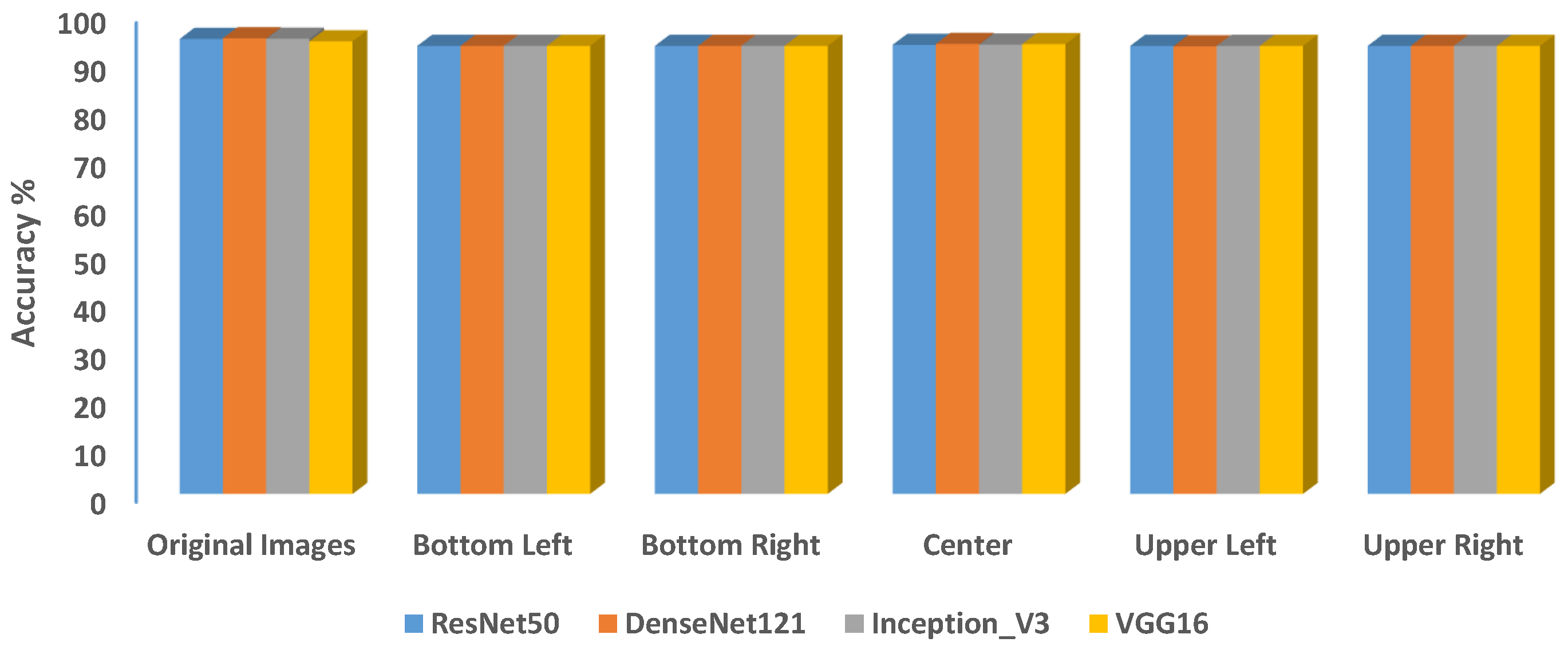
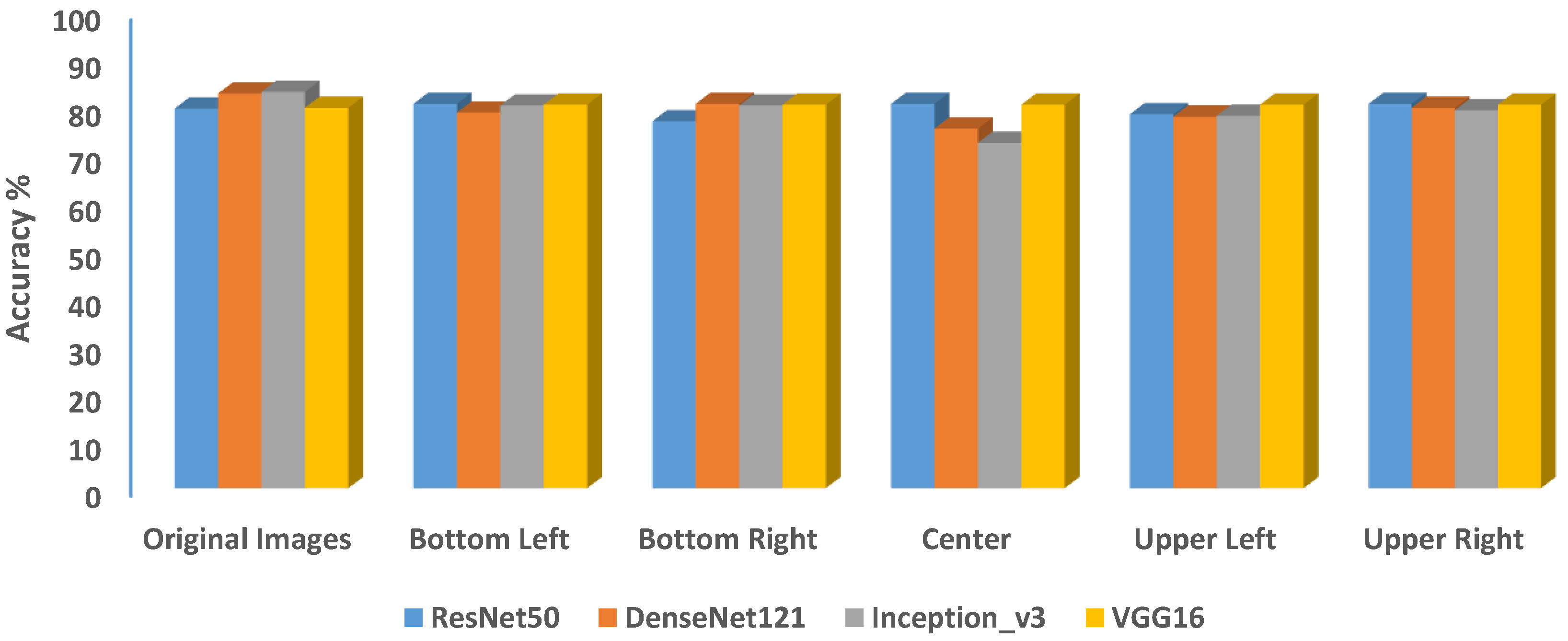
Surprisingly, all CNN models can also identify positive and negative cases across the cropped-image datasets, with an accuracy very close to that achieved by the original images. The results are shown in Figure 5. Furthermore, all CNN models achieved a consistent accuracy score of ∼93.42% across the cropped-image datasets, except for the center image datasets. Here, performance varied across CNN models and was slightly higher than their performance on the corresponding cropped images datasets.

The results reveal that the classification accuracy is consistently biased across the four corners crops (bottom-left, bottom-right, Upper-left, and upper-right). That is, cancer can be identified even when it is clear that the images do not include any medically relevant information. This suggests that the neural networks identify the presence of the disease not merely through clinical information, but also from other pieces of information and artifacts that might be linked to the way the datasets were collected rather than the clinical condition of the patient. Therefore, the classification accuracy observed when using CNNs to identify cancer might be overoptimistic, and not a direct reflection of the CNN models to automatically identify cancer.

In contrast to the small corner patches, the performance varied across all CNN models on the center images. This reflects the structural characteristics of the dataset, where the corners are generally uniform and homogeneous, while the center often contains lesion content. However, as shown through the corner patches, even in the absence of lesion structures in the cropped-image datasets, classification accuracy remained high.

3.1.3. NoduleMNIST (CT Scan Imaging)

NodueMNIST [54] dataset consists of thoracic CT scan slices. The images are centered on lung nodules labeled for binary classification (benign and malignant cases). The images show high contrast between lung functional tissues and surrounding tissues. If present, nodules are typically centered in the field of view. This is due to standardized radiology workflow and processing, ensuring the lesion is in view. We extracted cropped-image datasets from the original images. The resulting datasets consist of small images that are too visually subtle to contain any medical content to the unaided eye, as shown in Figure 3.

The performance across all models when using the original images is between ∼87.1% and ∼84.84%, achieved by DenseNet121 and VGG16, respectively. When using the five cropped-image datasets, the performance was well above mere chance, as shown in Figure 6. The performance observed with the patches taken from the center of each image closely matched those of the original images. In a particular instance, it was slightly higher than the original images. For example, VGG16 achieved a performance of ∼84.84% and ∼85.81% on original and center images, respectively. That shows that these architectures can identify cancer without medical information.

While the high performance by CNN models on full CT images can be expected, it is surprising that CNN architectures can also accurately classify the cropped images. The classification accuracy observed when using patches taken from the center of the images is higher than the accuracy observed with patches taken from the corner of the images. This could be linked to the spatial structure of the image, where center-cropped images may contain parts of the nodule, while corner patches mostly contain only background lung tissues. These cropped-image datasets do not contain medical information that is diagnostically relevant to an expert radiologist. This suggests that deep neural networks may rely on positional cues rather than learning from pathology-specific features.

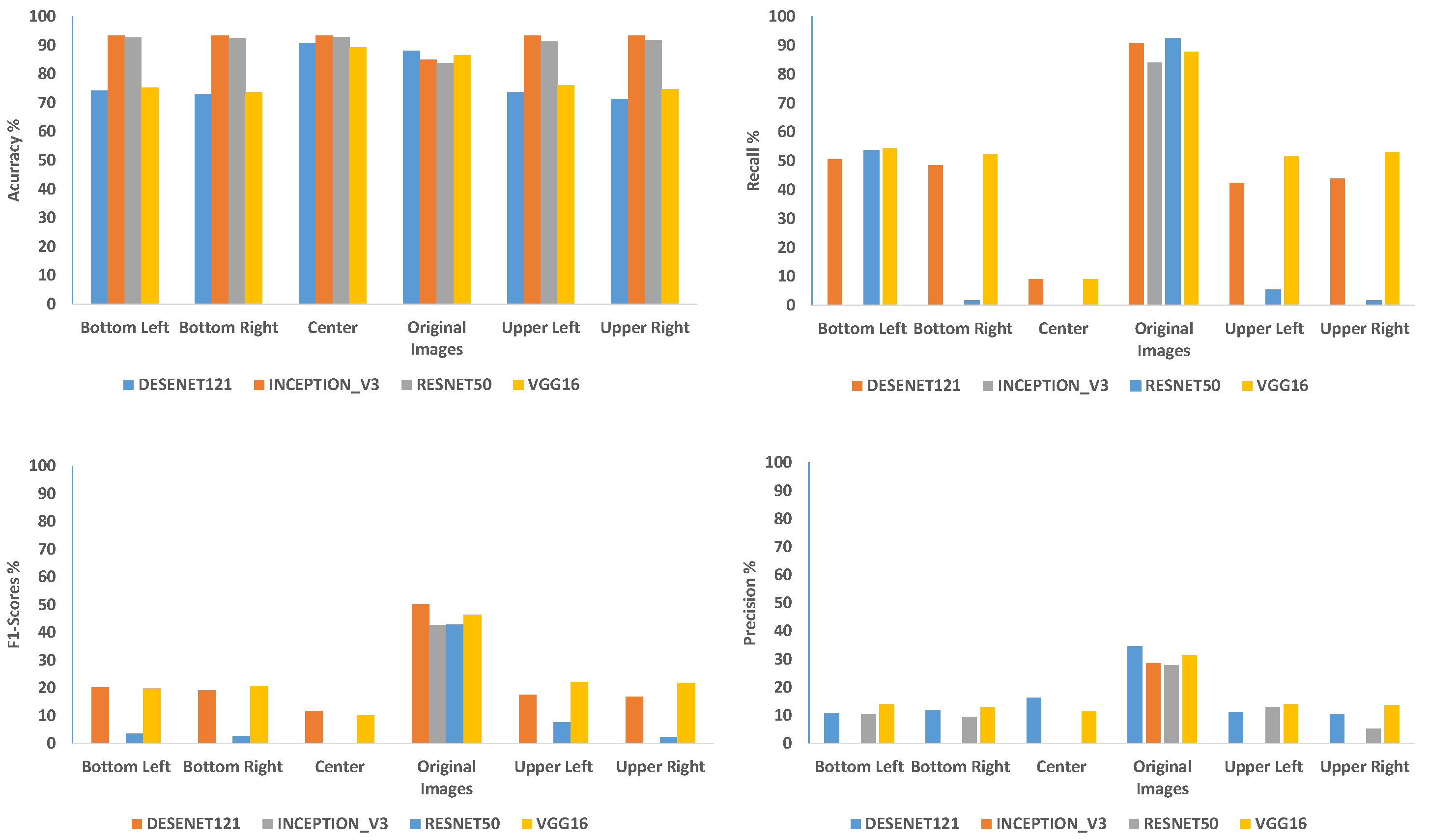
Another experiment was performed where the number of images in each class was equal, and set to 458. Figure 7 shows the classification accuracy, precision, recall and F-1 scores when each class contains exactly 458 images. The training and testing used the same settings as all other experiments. As the figure shows, the classification accuracy is far higher than mere chance. Even when using the background patches, the classification accuracy was, in many cases, higher than 90%.

3.1.4. PathMNIST (Histopathology Slides Imaging)

PathMNIST [51] consists of colored histopathology whole-slide images (WSIs) of colorectal cancer tissues. Each image is a single patch of tissue stained with hematoxylin and eosin (H&E). The generation and digitization of these WSIs are achieved using a standardized microscopy workflow in clinical labs. The images exhibit consistent staining, color balance, and pattern textures across the same class.

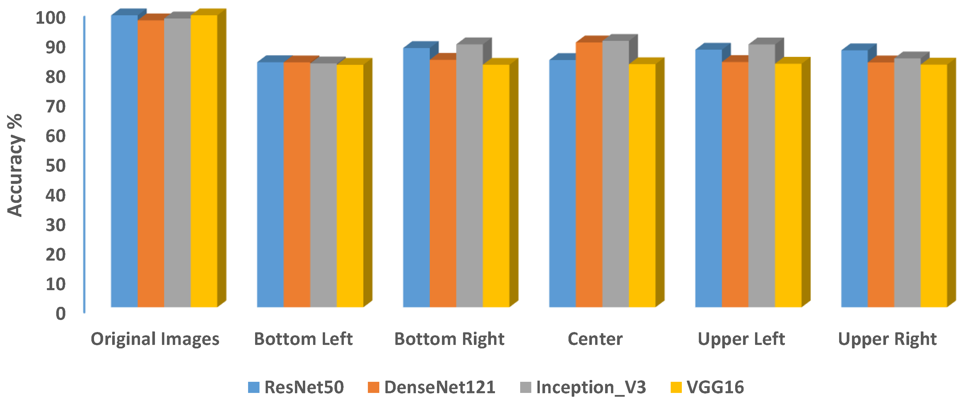
The results of the experiment on the original histopathology images, as expected, show that CNNs can classify the images with an accuracy as high as ∼98.72%. Figure 8 shows the results when the experiment was performed on the cropped-image datasets. InceptionV3 achieved an accuracy performance as high as ∼90.07% on the center-cropped images, while VGG16 achieved the lowest performance of ∼81.98% on the bottom-left cropped images.

The results of the experiments reveal that CNN models can identify positive cases even when using small patches from the corner of the images. A possible explanation for this is that cropped images retain color and texture features that correlate with class labels, even when they lack disease-related features. This may affect the model’s performance in real-world clinical settings, where test data may differ in structure.

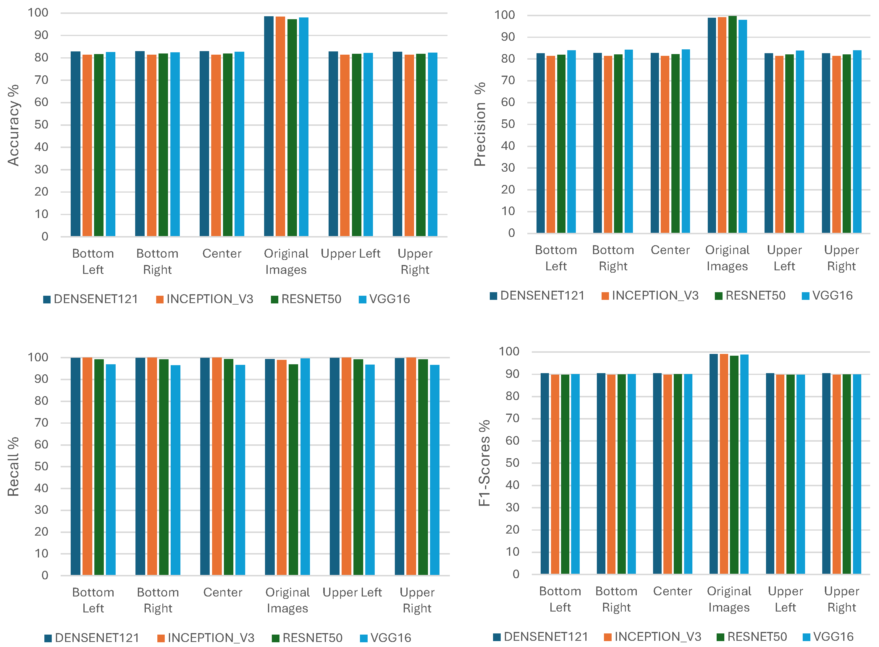
Figure 9 and

Table 6. Accuracy, precision, recall, and F-1 results of the analysis of the balanced PathMNIST.

Model	Sub Dataset	Accuracy	Recall	F-1	Precision
DENSENET121	Original Images	98.5376	98.8588	99.3495	99.1036
DENSENET121	Bottom Left	82.7994	82.6044	99.8973	90.4315
DENSENET121	Bottom Right	82.8830	82.6653	99.9144	90.4751
DENSENET121	Center	82.9109	82.6795	99.9315	90.4906
DENSENET121	Upper Left	82.7994	82.5952	99.9144	90.4330
DENSENET121	Upper Right	82.7855	82.6481	99.7946	90.4156
INCEPTION_V3	Original Images	98.4540	99.1425	98.9558	99.0491
INCEPTION_V3	Bottom Left	81.3649	81.3649	100	89.7251
INCEPTION_V3	Bottom Right	81.3649	81.3649	100	89.7251
INCEPTION_V3	Center	81.3928	81.3876	100	89.7389
INCEPTION_V3	Upper Left	81.3788	81.3762	100	89.7320
INCEPTION_V3	Upper Right	81.3649	81.3649	100	89.7251
RESNET50	Original Images	97.2423	99.6656	96.9360	98.2818
RESNET50	Bottom Left	81.6435	81.9582	99.2982	89.7988
RESNET50	Bottom Right	81.8524	82.1413	99.2811	89.9016
RESNET50	Center	81.9916	82.2122	99.3667	89.9791
RESNET50	Upper Left	81.7270	82.0187	99.3153	89.8421
RESNET50	Upper Right	81.7827	82.1378	99.1784	89.8573
VGG16	Original Images	97.9944	97.9307	99.6405	98.7782
VGG16	Bottom Left	82.5209	84.0231	96.9531	90.0262
VGG16	Bottom Right	82.4373	84.2223	96.4909	89.9402
VGG16	Center	82.6602	84.2804	96.7306	90.0773
VGG16	Upper Left	82.2006	83.8275	96.7990	89.8475
VGG16	Upper Right	82.2563	83.9578	96.6621	89.8631

show the classification accuracy, precision, recall and F-1 scores when the number of images in each class is equal, and set to 9366. The results shows that all architectures could identify cancer with an accuracy much higher than mere chance, and the classification accuracy in all cases was higher than 80%.

3.2. CNNs and BreakHis Datasets (Histopathology Imaging)

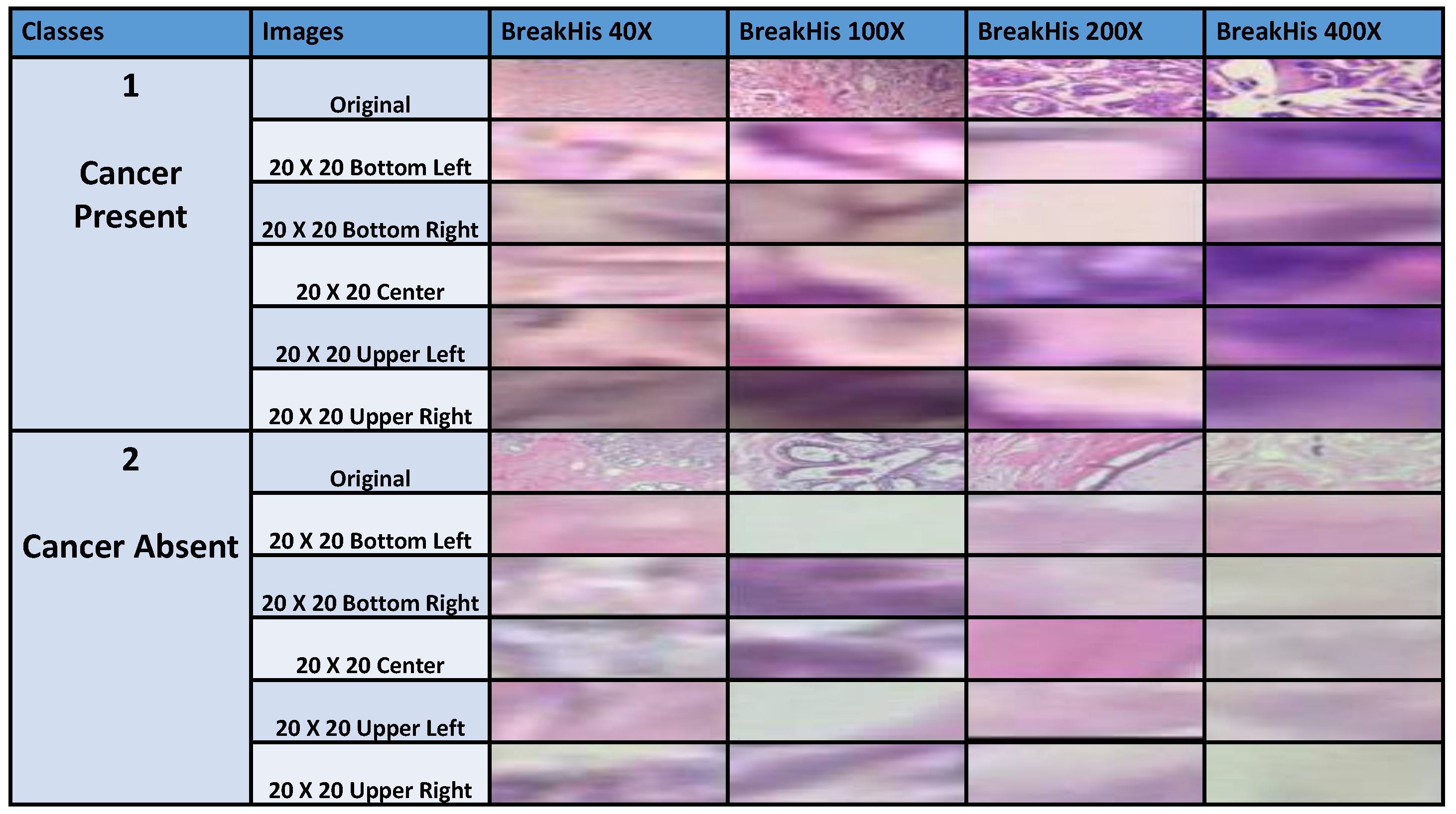
In the BreakHis datasets, at a specific magnification level, each image displays tissue structure divided into benign and malignant classes. Images are similar at each magnification level, with consistent color stains and background patterns. Here, lesions may not be centered, and the images contain mainly lesions and background, as shown in Figure 10.

We evaluated the classification performance of the four CNN models (ResNet50, DenseNet121, InceptionV3, and VGG16) on the BreakHis datasets across the four magnification levels ($40\times$, $100\times$, $200\times$, and $400\times$). The experiment was first performed on the original image dataset and then on the cropped-image datasets. The cropped-image datasets were generated by extracting five 20 × 20 pixel sections from the original images. Each cropped dataset (bottom-left, bottom-right, center, upper-left, and upper-right) contains images that are too small to contain any meaningful tissue structure for pathology analysis.

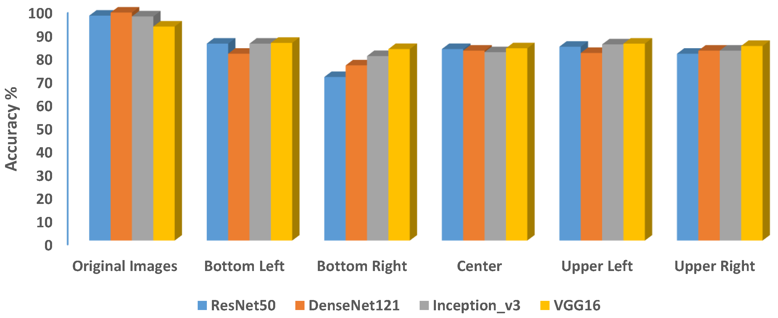
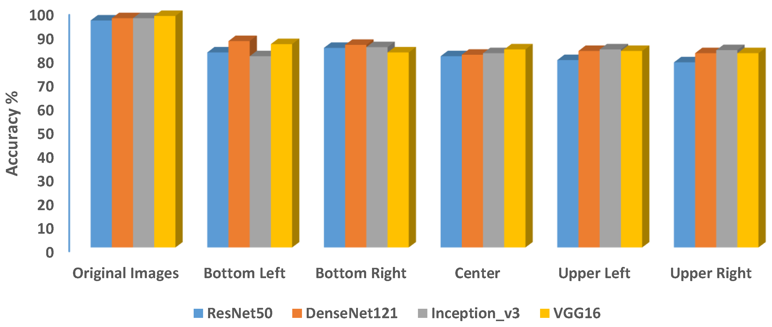
The results revealed the same pattern across all magnification levels. Figure 11, Figure 12, Figure 13 and Figure 14 show the results from each magnification level of $40\times$, $100\times$, $200\times$, and $400\times$, respectively.

Table 7. Summary of the results of the analysis of the BreakHis dataset with 40× magnification.

Model	Sub Dataset	Accuracy	Recall	F-1	Precision
DENSENET121	Original Images	97.69	97.97	98.30	98.64
DENSENET121	Bottom Left	55.48	51.58	49.49	64.49
DENSENET121	Bottom Right	55.35	50.48	48.87	65.09
DENSENET121	Center	56.41	52.64	50.93	84.84
DENSENET121	Upper Left	55.93	52.25	50.27	85.12
DENSENET121	Upper Right	54.74	49.95	48.53	65.76
INCEPTION_V3	Original Images	97.12	97.45	97.90	98.37
INCEPTION_V3	Bottom Left	69.08	92.23	80.13	71.81
INCEPTION_V3	Bottom Right	68.27	90.87	79.29	71.58
INCEPTION_V3	Center	69.14	91.79	80.05	71.89
INCEPTION_V3	Upper Left	68.00	90.88	79.14	71.50
INCEPTION_V3	Upper Right	68.03	90.08	78.99	71.85
RESNET50	Original Images	96.06	96.63	97.12	97.66
RESNET50	Bottom Left	57.43	57.72	60.75	77.25
RESNET50	Bottom Right	56.04	54.53	58.46	77.37
RESNET50	Center	57.99	58.94	61.45	77.00
RESNET50	Upper Left	57.30	57.09	60.91	77.40
RESNET50	Upper Right	55.16	52.54	57.09	77.34
VGG16	Original Images	95.15	94.80	96.35	98.01
VGG16	Bottom Left	72.18	99.79	83.22	71.38
VGG16	Bottom Right	72.66	99.67	83.45	71.79
VGG16	Center	72.19	99.75	83.21	71.39
VGG16	Upper Left	71.65	99.83	82.95	70.97
VGG16	Upper Right	72.22	99.71	83.22	71.43

summarizes the results for the 40× magnification.

In these results, the CNN models are shown to be able to classify the original images with an accuracy as high as $95\%$. The results also show that CNNs can identify the classes in the cropped-image datasets with a classification accuracy as high as $88\%$. Achieving a classification accuracy well above that of mere chance, $50\%$, when using the cropped images is unexpected.

The consistent ability of deep neural networks to correctly classify the cropped images across all magnification levels suggests potential bias. Each CNN model can identify class-unique features even when the images contain no visible tissue samples. Deep neural networks may exploit location-based features rather than the generalized learning of disease characteristics. This may occur if certain histological patterns, staining colors, or texture features are consistently present in specific regions of the slides. This raises concerns about the reliability of CNN performance in real-world clinical settings in situations where the tissue presentation of the test distribution may differ from the training distribution.

Another experiment was performed to test the effect of class balancing. Figure 15 shows the classification accuracy, precision, recall and F-1 scores of the 40× magnification of the BreakHis images. Each class contained 405 images, and the training and testing were carried out using the same settings as the other experiments. As the figure shows, the architectures are still able to identify cancer with an accuracy much higher than mere chance, with the classification accuracy of the original images being close to 100%, and the background patches provide an accuracy of 70–80% for most architectures.

3.3. CNN and ISIC Datasets (Dermoscopic Lesion Skin Imaging)

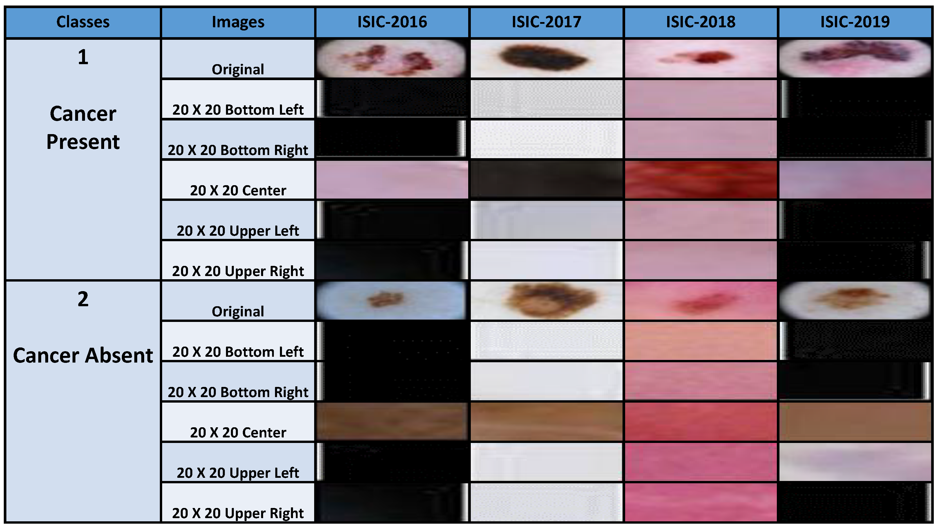
The application of deep neural networks for the classification of dermoscopic images is standard practice. However, when we extract 20 × 20 cropped images from the ISIC original images (four corners and the center), CNNs are not expected to identify cancerous and non-cancerous lesions. These cropped images contain black or skin-toned backgrounds that are not related to the disease pathology. In some cases, the center-cropped images contain pigmentation that is diagnostically meaningless to an expert dermatologist. Figure 16 shows sample images of the original images and their corresponding 20 × 20 cropped images across the ISIC datasets.

Despite this, the results of the experiments across ISIC datasets (ISIC-2016 to ISIC-2019) show that CNNs can distinguish malignant from benign cases in these cropped images. In some cases, CNNs achieved a marginally higher accuracy score on the cropped images than on the original images.

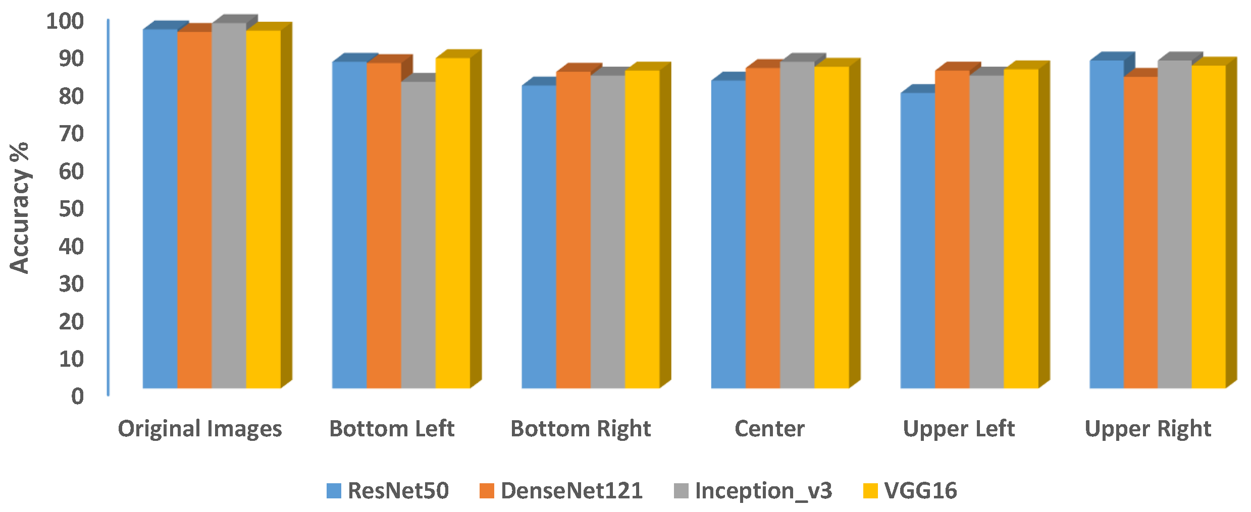
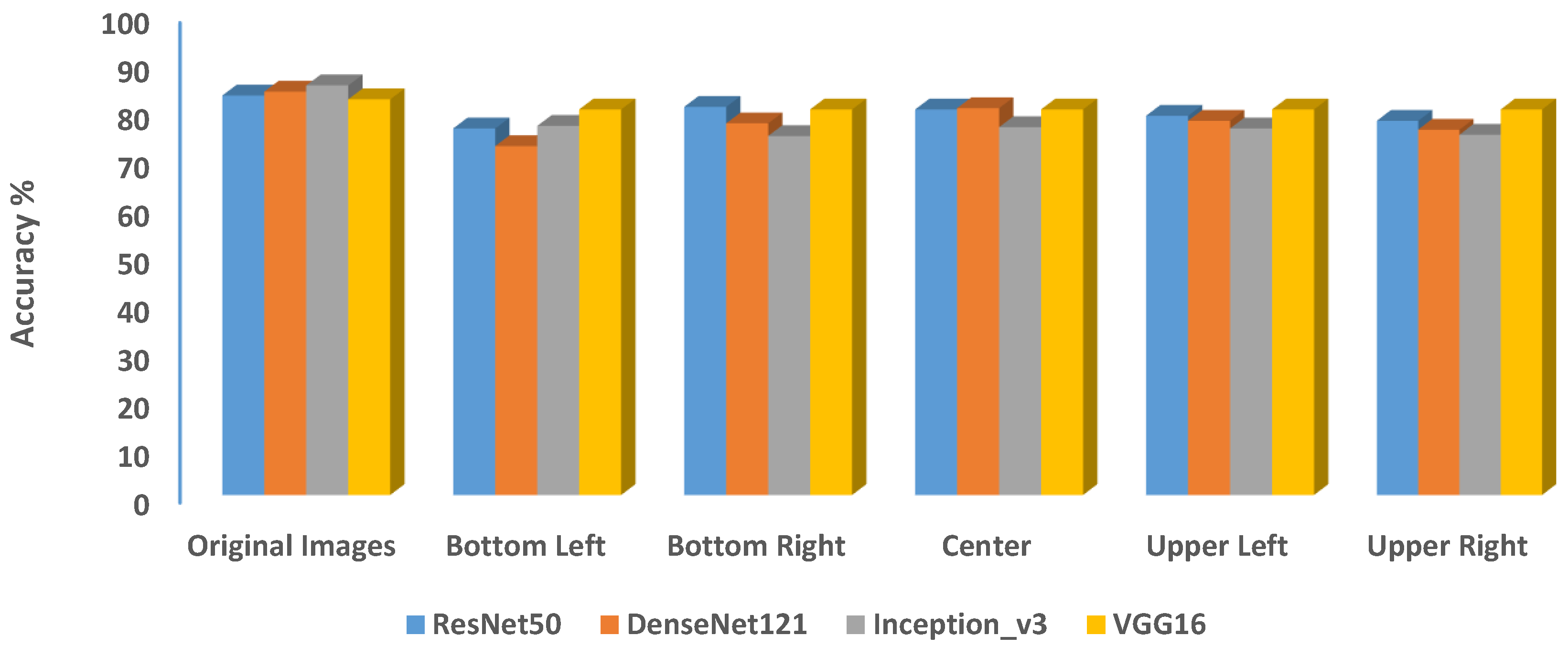
For example, VGG16 exhibited a consistent accuracy performance of ∼80.5% across all cropped images datasets of ISIC-2017, as shown in Figure 17. This performance is slightly higher than the performance of ∼79.83% it achieved on the original images. ResNet50 also showed a similar trend by achieving a consistent accuracy score of ∼80.67% for bottom-left, center-, and upper-right cropped images, which is slightly higher than the accuracy it achieved on the original images.

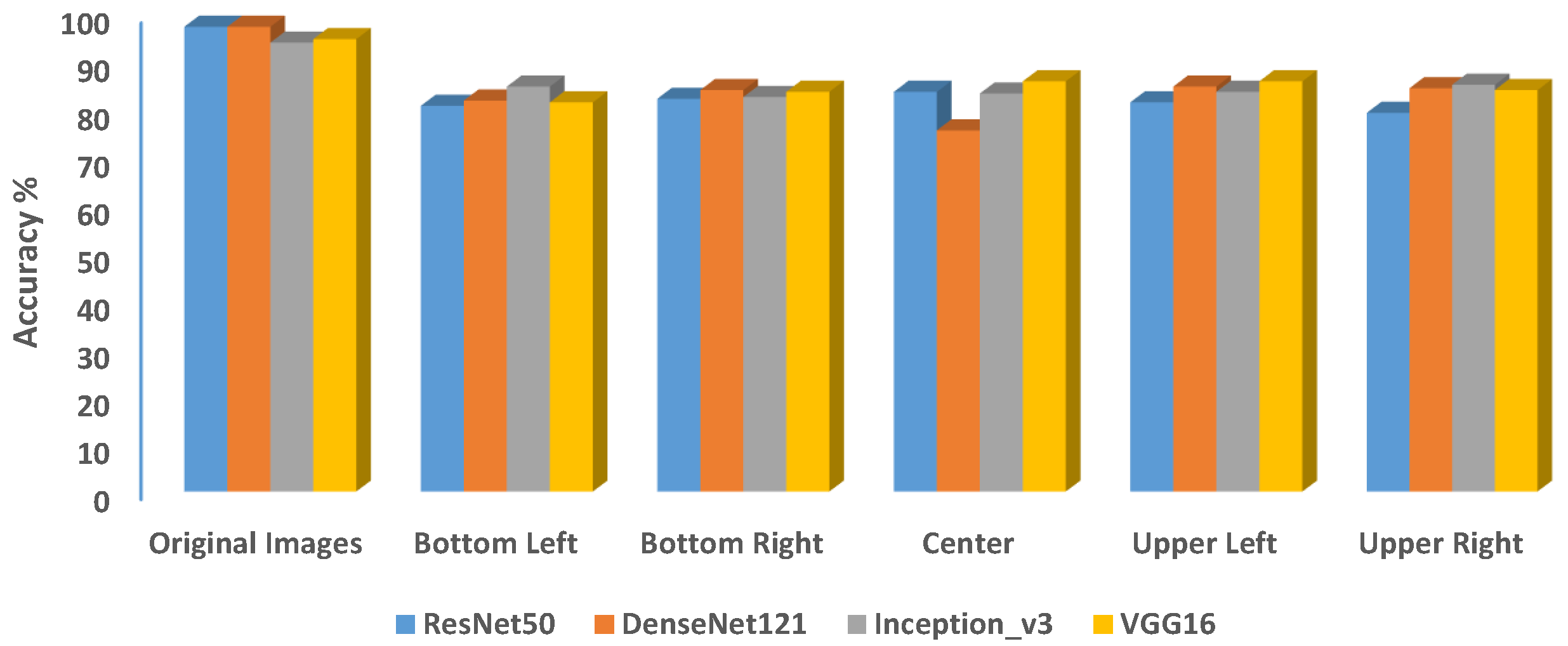
As shown in Figure 18, VGG16 also achieved a consistent accuracy performance of ∼80.21% when applied to all the cropped-image datasets of ISIC-2016, in contrast to its performance on the ISIC-2017 dataset, where it achieved a slightly lower performance than that achieved on the original images.

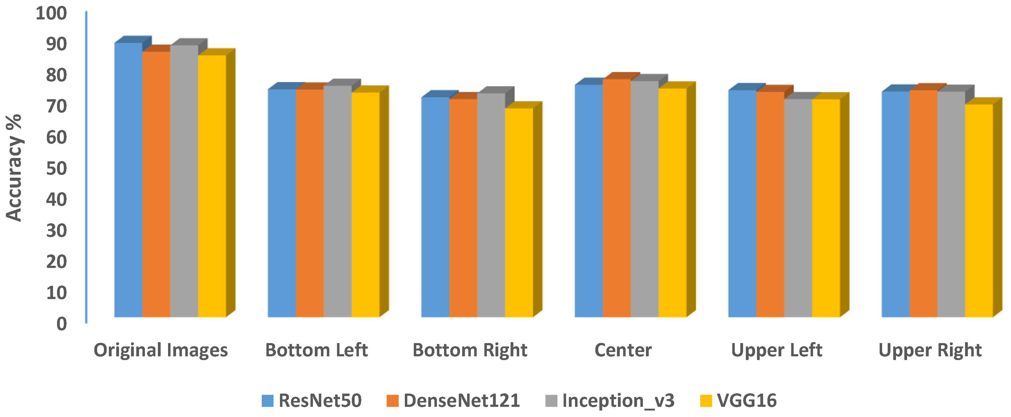
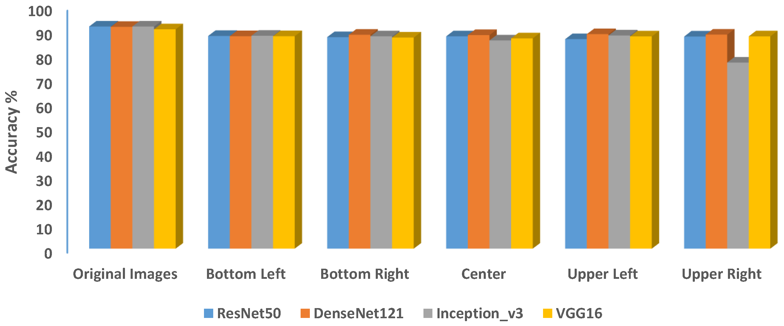
Another dataset we tested is the ISIC-2018. The results also reveal the ability of CNN models to identify classes from the cropped images. However, the margin between the performance across models on the original images and the cropped-image datasets increased. This suggests little resistance to potential bias compared to the results from previous years (ISIC-2016 and ISIC-2017). For example, Figure 19 shows that deep neural networks can classify both the original and cropped images with accuracy as high as ∼88.29% and ∼76.57%, respectively.

Table 8. Accuracy, precision, recall, and F-1 results of the analysis of the balanced ISIC-2018 dataset.

Model	Sub Dataset	Accuracy	Recall	F-1	Precision
DENSENET121	Original Images	85.8372	85.5634	81.9552	78.7535
DENSENET121	Bottom Right	62.8590	4.4366	7.4707	28.3412
DENSENET121	Bottom Left	62.7399	3.9437	6.8230	35.0489
DENSENET121	Center	61.2442	6.5141	10.0572	64.2105
DENSENET121	Upper Left	62.9782	4.6479	7.9069	57.9132
DENSENET121	Upper Right	62.8855	4.7887	7.9559	42.9699
INCEPTION_V3	Original Images	84.8312	84.7887	80.8230	77.6369
INCEPTION_V3	Bottom Right	62.6208	2.8169	4.5410	41.0638
INCEPTION_V3	Bottom Left	62.7796	2.6761	4.5365	24.9397
INCEPTION_V3	Center	62.2766	2.3592	4.1722	19.4480
INCEPTION_V3	Upper Left	62.7929	2.5000	4.2595	29.0031
INCEPTION_V3	Upper Right	62.7929	2.6761	4.5215	25.6140
RESNET50	Original Images	85.1621	83.2042	80.8063	78.8106
RESNET50	Bottom Right	63.0443	6.9014	11.4470	58.2067
RESNET50	Bottom Left	63.0841	5.8451	9.9479	44.7500
RESNET50	Center	61.7737	1.6197	2.8298	13.2013
RESNET50	Upper Left	63.6929	8.2042	13.4575	57.7125
RESNET50	Upper Right	63.6664	7.9930	13.1650	68.3775
VGG16	Original Images	82.9385	82.4296	78.4074	74.9589
VGG16	Bottom Right	63.0311	7.9930	11.7898	42.2358
VGG16	Bottom Left	63.0179	7.2183	10.9649	32.5476
VGG16	Center	62.8326	6.6549	11.3717	62.9896
VGG16	Upper Left	63.3091	7.8521	11.8730	63.5431
VGG16	Upper Right	63.2694	7.6056	11.5838	53.5498

shows the classification accuracy. precision, recall and F-1 scores of the ISIC-2018 dataset when the classes are balanced. As before, different parts of each image are used. As the table shows, in all cases the classification accuracy is higher than mere chance-based accuracy, even when using sub-images with no medical information. The classification accuracy is consistent across different parts of the images at around 63%.

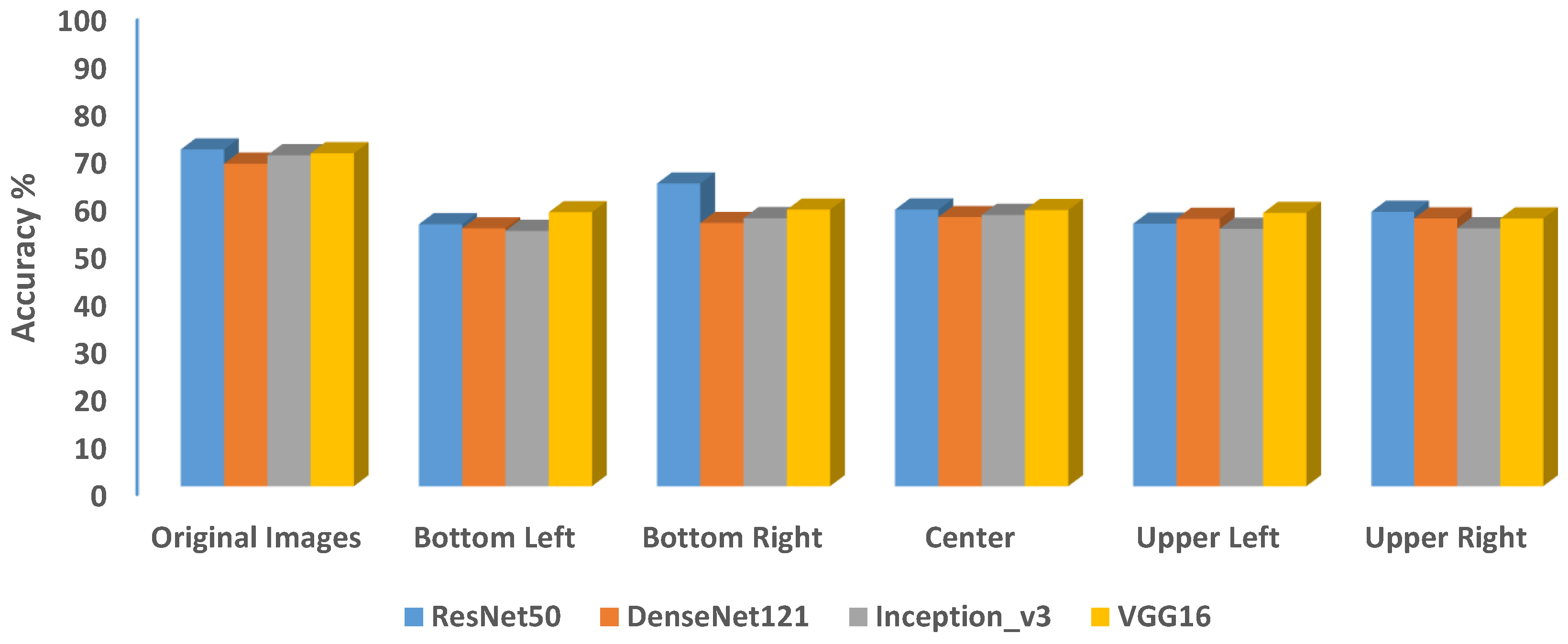
When the experiment was performed on the ISIC-2019 dataset, the results reveal a significant drop in overall performance. All CNN architectures achieved lower accuracy scores compared to previous years, both on the original and cropped-image datasets. The performance of the models on the original images is between ∼70.93% and ∼67.93%, with these results achieved by ResNet50 and DenseNet121, respectively. Most CNN models showed a moderate performance when applied to the cropped-image datasets. In most cases, performance was only slightly higher than that of mere chance, 50%. InceptionV3 achieved the lowest performance of ∼54.33% and ResNet50 achieved the maximum performance of ∼63.75%, as shown in Figure 20. This shows that these results might be less subjected to bias.

Table 9. Accuracy, precision, recall, and F-1 results of the analysis of the balanced ISIC-2019 dataset.

Model	Sub Dataset	Accuracy	Recall	F-1	Precision
DENSENET121	Original Images	0.68	0.53	0.78	0.63
DENSENET121	Bottom Left	0.48	0.38	0.80	0.52
DENSENET121	Bottom Right	0.48	0.38	0.82	0.52
DENSENET121	Center	0.48	0.30	0.40	0.34
DENSENET121	Upper Left	0.48	0.38	0.82	0.52
DENSENET121	Upper Right	0.49	0.39	0.84	0.53
INCEPTION_V3	Original Images	0.68	0.53	0.80	0.64
INCEPTION_V3	Bottom Left	0.41	0.35	0.84	0.50
INCEPTION_V3	Bottom Right	0.43	0.36	0.85	0.51
INCEPTION_V3	Center	0.46	0.37	0.78	0.50
INCEPTION_V3	Upper Left	0.45	0.37	0.85	0.52
INCEPTION_V3	Upper Right	0.44	0.37	0.85	0.51
RESNET50	Original Images	0.67	0.51	0.84	0.63
RESNET50	Bottom Left	0.55	0.40	0.67	0.50
RESNET50	Bottom Right	0.54	0.40	0.66	0.50
RESNET50	Center	0.52	0.31	0.31	0.31
RESNET50	Upper Left	0.55	0.40	0.67	0.51
RESNET50	Upper Right	0.55	0.40	0.66	0.50
VGG16	Original Images	0.61	0.46	0.90	0.61
VGG16	Bottom Left	0.57	0.41	0.58	0.48
VGG16	Bottom Right	0.56	0.41	0.62	0.49
VGG16	Center	0.64	0.37	0.05	0.09
VGG16	Upper Left	0.56	0.41	0.64	0.50
VGG16	Upper Right	0.55	0.41	0.67	0.51

shows the accuracy, precision, recall, and F-1 results when the classes are balanced. As with the previous experiments with that dataset, the classification accuracy using the background sub-images with no medical information, in most cases, was approximately the same as the expected accuracy when using only chance. These results are not necessarily surprising, given the results shown in Figure 20.

The results across all datasets (ISIC-201 to ISIC-2017) indicate that neural networks may be learning from irrelevant background features in the original images. This may influence their ability to classify images lacking disease-related features. In later years (ISIC-2018 and ISIC-2019), the noticeable drop in the performance of CNN on the cropped-image datasets points to reduced susceptibility to bias compared to the results from previous years. This indicates that the bias in the performance of deep neural networks may be related to the complexity of biomedical image datasets.

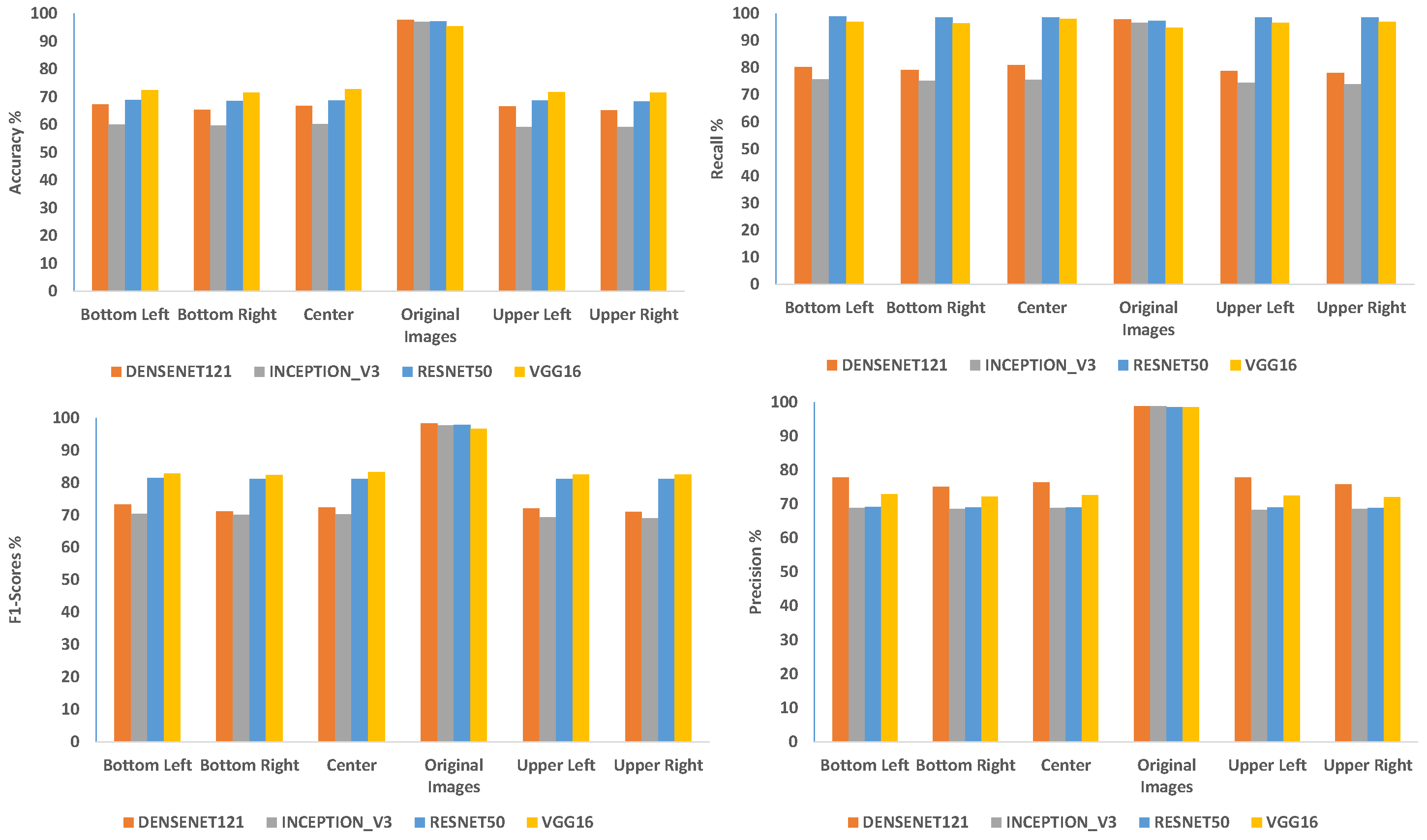
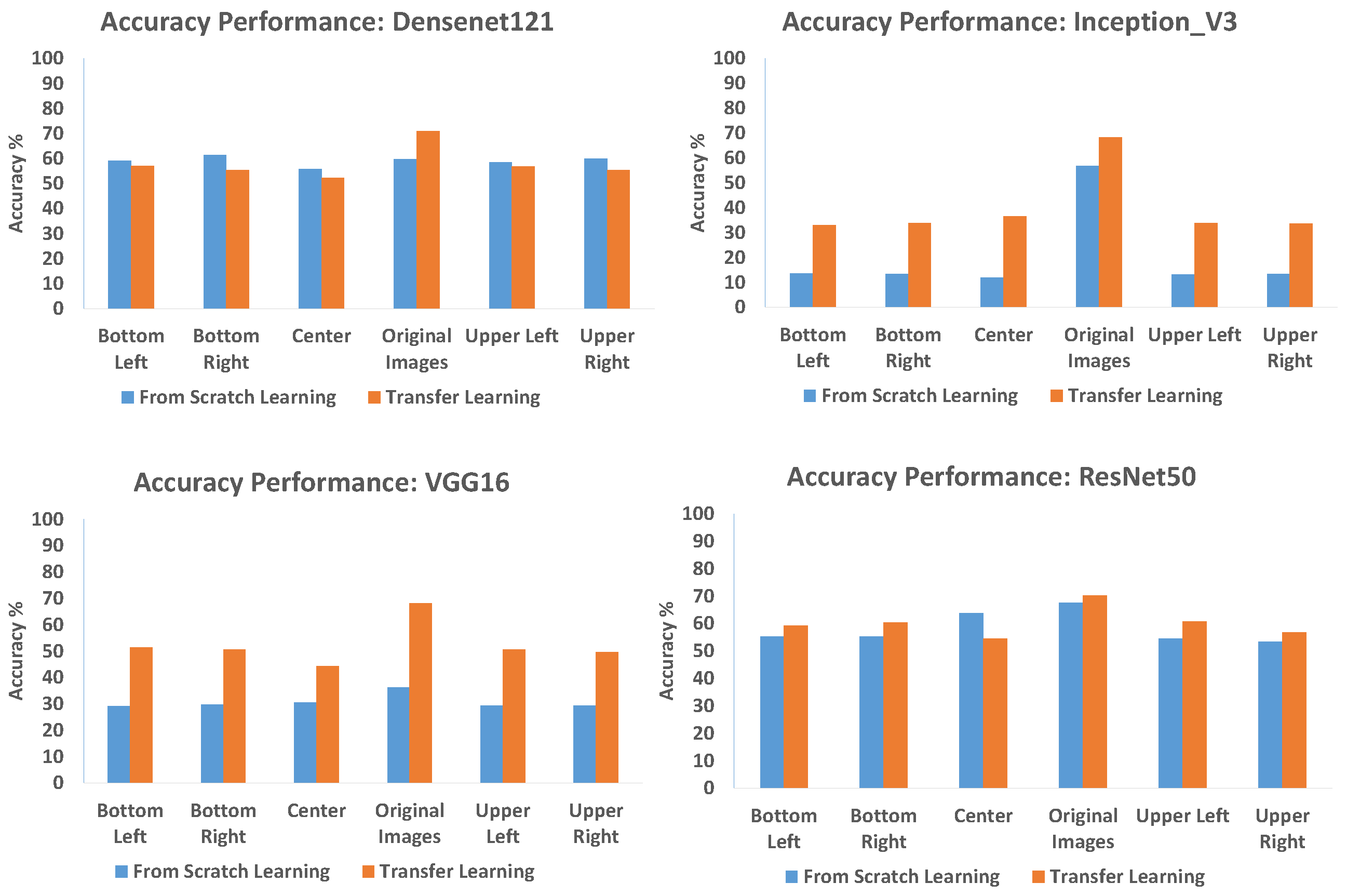
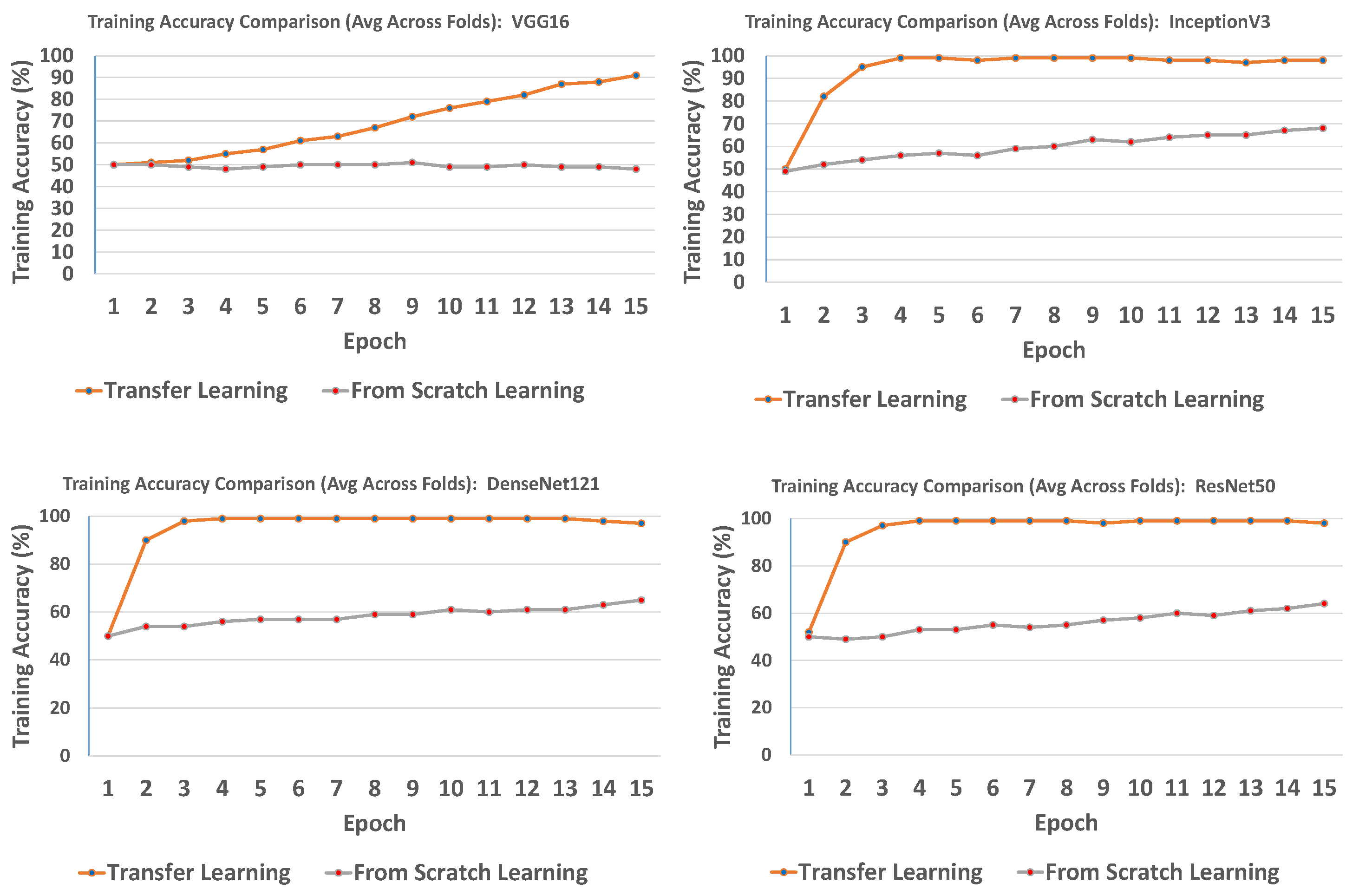
We also used ISIC to test the effect of transfer learning. Transfer learning is the standard practice for training deep neural networks, and therefore the experiments above were performed with transfer learning. However, to test if the bias derived from the practice of transfer learning, we also tested ISIC-2016 with and without transfer learning. That was achieved by using 15 epochs when training with or without transfer learning to ensure that the only difference between the experiments was the use of transfer learning. Figure 21 shows the classification accuracy of the different parts with or without transfer learning. The analysis was carried out for the different CNNs architectures.

As the figure shows, transfer learning performed better when classifying the original images. That is expected, as transfer learning is known to improve the training; therefore, the common practice is to use transfer learning.

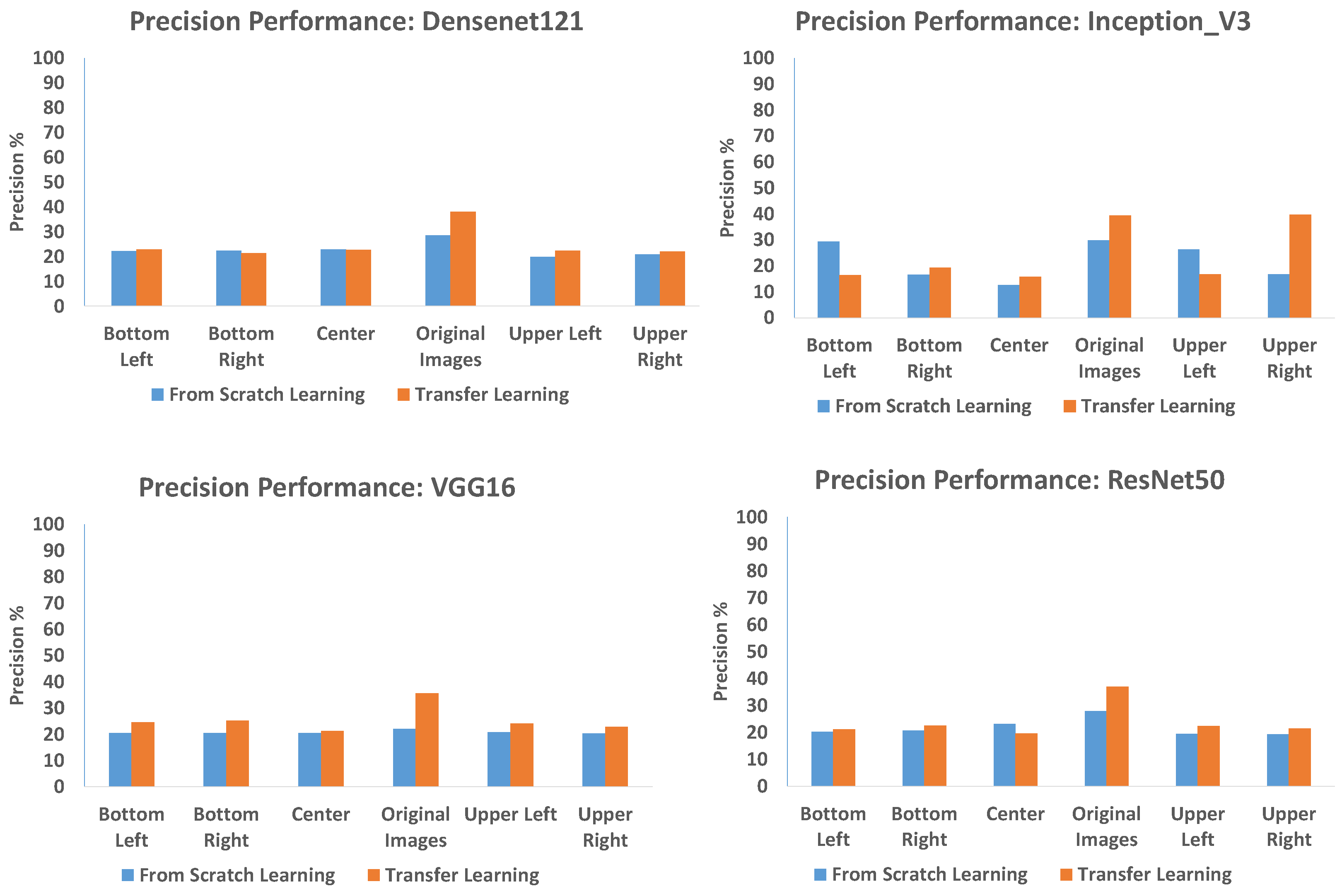
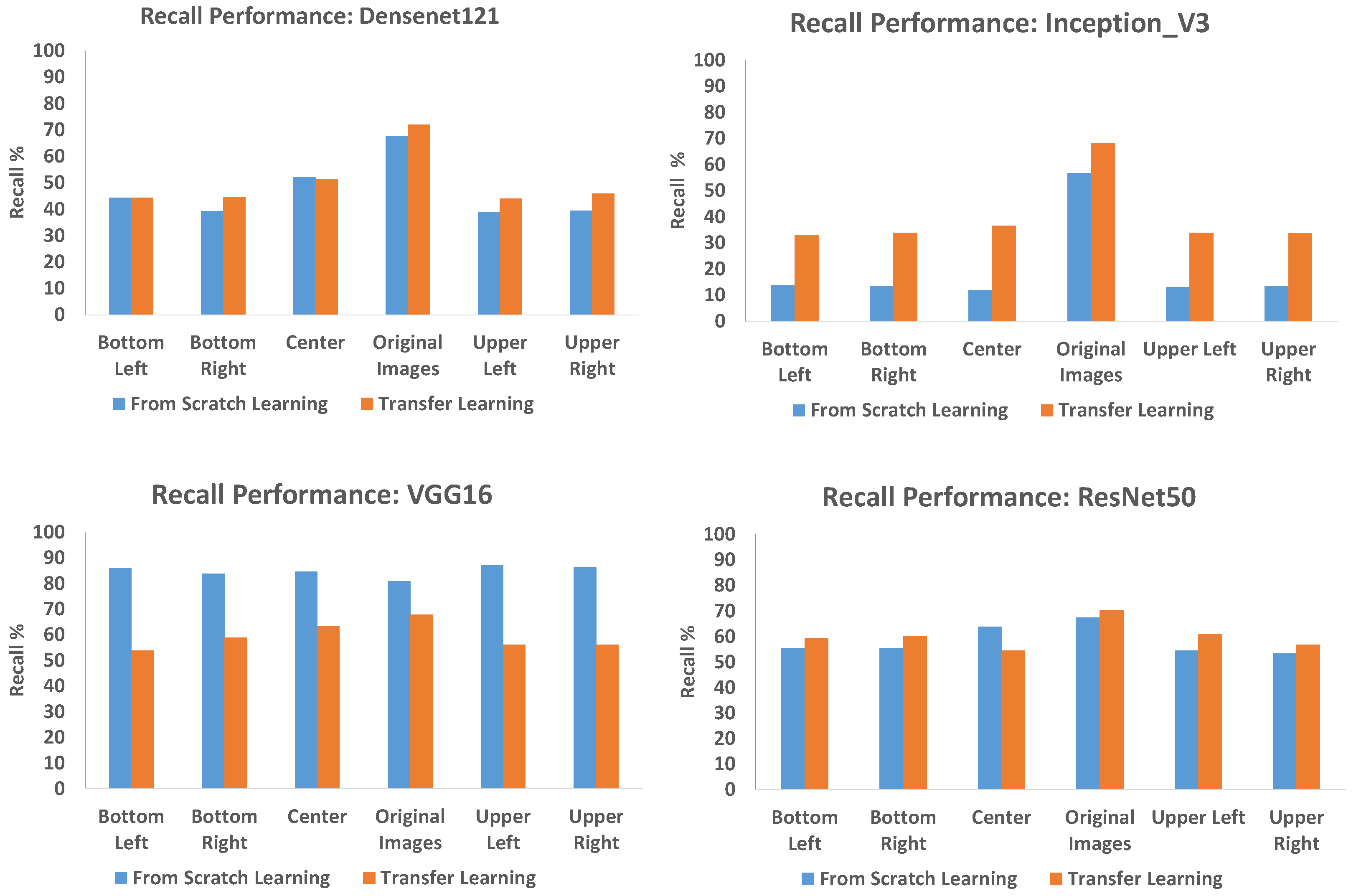
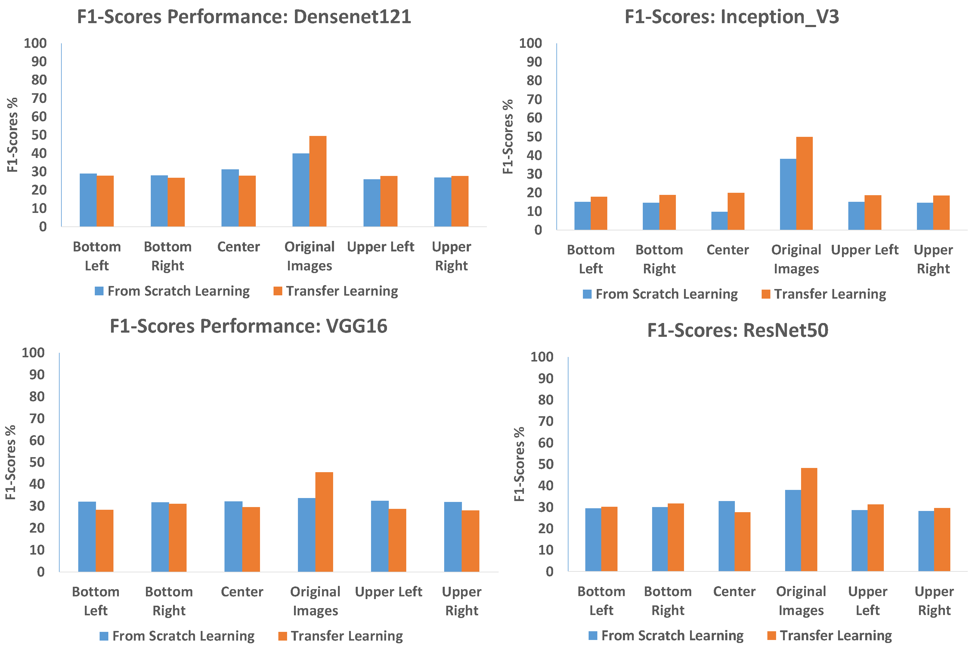
Interestingly, with the exception of VGG-16, the bias did not increase substantially when using transfer learning, and in the case of Inception V3 it even decreased. That shows that the bias is not driven by the information that is present in common natural images, but is specific to the image dataset. Figure 22, Figure 23 and Figure 24 show the precision, recall, and F-1 scores when using different parts of the images and different architectures.

Figure 25 shows the learning with different numbers of epochs for the different architectures. As expected, transfer learning makes the learning substantially faster compared to starting with random weights. For the deeper architectures such as Densenet-121 and Resnet-50, the difference between transfer learning and random weights is even more substantial.

3.4. CNN and Breast Histopathology Images for Invasive Ductal Carcinoma (IDC) Dataset (Histopathology Imaging)

The IDC datasets contain H&E-stained breast tissue slides of histopathology image tiles. Each image is labeled either cancerous or noncancerous, making them suitable for binary classification.

To test for bias, we further cropped each original image into 20 × 20 patches from five regions. These cropped-image datasets contain only plain tissues or small fractions of breast tissues, instead of the full cancer structure. The information contained in these cropped images is not sufficient for accurate diagnostics.

An accuracy score of above 89% was observed with all deep neural networks on the Breast Histopathology Image (IDC) original image dataset. However, all models also achieved far higher than the random accuracy across all cropped 20 × 20 subset datasets, with ResNet50 having showing the lowest performance of ∼85%, as shown in Figure 26. The ability of these CNN models to successfully identify the classes in the cropped images that do not contain sufficient clinical information shows that the results observed with the full images could be biased. These results are aligned with other histopathology image datasets, such as PathMNIST and BreakHis, as shown above.

4. Conclusions

CNNs have become a widely adopted tool for automatic pathology. Due to the availability of easy-to-use libraries, CNNs have become powerful tools for cancer pathology. This study highlights a weakness in the common practice of the use of CNNs for biomedical image analysis, unmasking their vulnerability to bias when applied to cancer diagnostics.

We examined whether deep neural networks learn solely from meaningful diagnostic features, or also rely on background details/dataset-specific artifacts. To investigate this, we evaluated the performance of four commonly used CNN models across thirteen diverse biomedical datasets. These datasets are widely used by machine learning experts and the medical AI community, representing different types of cancer and imaging modalities. We then compared the performance of each CNN model on the original image to that observed when using 20 × 20 pixel regions. These cropped images contain little or no medical content useful for meaningful diagnosis.

Surprisingly, the results across all datasets showed that CNNs consistently achieved an accuracy higher than random chance on the cropped image. In some cases, CNNs achieved a matching or better performance than that achieved the original images, even when the images lacked relevant diagnostic features. In other cases, the original images allowed for better classification accuracy compared to the small background sub-images, which is expected given that the original images are larger and therefore contain more information that allows for classification, including the medically relevant parts of the images. However, the fact that the background sub-images provided a classification accuracy that is better than random chance, despite containing no medically relevant information, shows that the CNN models did not solely learn from cancer-specific visual features during training. This effect cuts across all types of cancer and imaging modalities, underscoring that the bias issue is both widespread and modality-independent.

The findings show that CNNs make use of information that is not necessarily clinical to identify between the classes. Therefore, the results observed by applying CNNs to cancer pathology might be substantially biased, and do not necessarily represent the real ability of the CNN to identify cancer. While the use of CNN models on benchmark datasets appears promising, such performance may not reflect true pathology interpretation. This may pose a risk in critical medical contexts, such as cancer diagnosis, where incorrect diagnoses can have severe consequences.

Although this study exposes potential bias in the common practice of using deep neural networks for biomedical image analysis, it does not scientifically investigate the root causes of the bias. The analysis is limited to four CNN architectures and thirteen widely used biomedical image datasets. Although these architectures and benchmarks are commonly used, it is definitely possible that some benchmarks and architectures are not biased. The size of the sub-images is 20 × 20, which is based on previous experiments on datasets from other domains [27,31,33]. While other sizes could provide different results, the fact that classification accuracy can be observed with no medical information indicates the possible presence of bias. Since all images are processed in the same way, artifacts that are derived from the image processing should affect all classes equally, and therefore should not lead to differences between the classes.

Since CNNs are not intuitive, and work largely as a “black box”, interpretation of the sources of bias is not trivial, and requires understanding the conditions under which the benchmark datasets were prepared. That is, while the outcome of this experiment across all datasets revealed bias, the study did not explore why such bias exists or how it can be addressed.

Future research work will focus on profiling not merely the presence of bias, but also the reasons for it. That will involve collecting biomedical image datasets instead of relying on publicly available datasets. Control over the image acquisition process will allow for the proper documentation of relevant clinical variables such as temperature, camera settings, staining protocols, lighting, and acquisition devices during image processing and clinical workflow. This creates the possibility for researchers to systematically analyze how these clinical and acquisition factors contribute to CNN model bias.

Furthermore, this will serve as a foundation for developing methods for reducing or totally mitigating such bias in the use of deep neural networks for cancer diagnosis. That will be achieved using explainable AI tools and engineered features such as textures or polynomial decomposition of the images, as well as common tools such as saliency maps.

References

1. Echle, A.; Rindtorff, N.T.; Brinker, T.J.; Luedde, T.; Pearson, A.T.; Kather, J.N. Deep learning in cancer pathology: A new generation of clinical biomarkers. Br. J. Cancer 2021, 124, 686–696. [Google Scholar] [CrossRef] [Scilit]
2. Zhu, X.; Yao, J.; Huang, J. Deep convolutional neural network for survival analysis with pathological images. In Proceedings of the 2016 IEEE International Conference on Bioinformatics and Biomedicine (BIBM); IEEE: Piscataway, NJ, USA, 2016; pp. 544–547. [Google Scholar]
3. Orlov, N.V.; Chen, W.W.; Eckley, D.M.; Macura, T.J.; Shamir, L.; Jaffe, E.S.; Goldberg, I.G. Automatic classification of lymphoma images with transform-based global features. IEEE Trans. Inf. Technol. Biomed. 2010, 14, 1003–1013. [Google Scholar] [CrossRef] [Scilit] [PubMed]
4. Xiao, M.; Li, Y.; Yan, X.; Gao, M.; Wang, W. Convolutional neural network classification of cancer cytopathology images: Taking breast cancer as an example. In Proceedings of the 2024 7th International Conference on Machine Vision and Applications, Singapore, 12–14 March 2024; pp. 145–149. [Google Scholar]
5. Xu, Y.; Khan, T.M.; Song, Y.; Meijering, E. Edge deep learning in computer vision and medical diagnostics: A comprehensive survey. Artif. Intell. Rev. 2025, 58, 93. [Google Scholar] [CrossRef] [Scilit]
6. Ciga, O.; Xu, T.; Martel, A.L. Self supervised contrastive learning for digital histopathology. Mach. Learn. Appl. 2022, 7, 100198. [Google Scholar] [CrossRef] [Scilit]
7. De Matos, J.; Ataky, S.T.M.; de Souza Britto, A., Jr.; Soares de Oliveira, L.E.; Lameiras Koerich, A. Machine learning methods for histopathological image analysis: A review. Electronics 2021, 10, 562. [Google Scholar] [CrossRef] [Scilit]
8. Rajadurai, S.; Perumal, K.; Ijaz, M.F.; Chowdhary, C.L. Precisionlymphonet: Advancing malignant lymphoma diagnosis via ensemble transfer learning with cnns. Diagnostics 2024, 14, 469. [Google Scholar] [CrossRef] [Scilit] [PubMed]
9. Chen, H.; Li, X.; Li, C.; Rahaman, M.M.; Li, X.; Wu, J.; Sun, H.; Grzegorzek, M.; Li, X. What can machine vision do for lymphatic histopathology image analysis: A comprehensive review. Artif. Intell. Rev. 2024, 57, 71. [Google Scholar] [CrossRef] [Scilit]
10. Shen, D.; Wu, G.; Suk, H.I. Deep learning in medical image analysis. Annu. Rev. Biomed. Eng. 2017, 19, 221–248. [Google Scholar] [CrossRef] [Scilit] [PubMed]
11. Irede, E.L.; Aworinde, O.R.; Lekan, O.K.; Amienghemhen, O.D.; Okonkwo, T.P.; Onivefu, A.P.; Ifijen, I.H. Medical imaging: A critical review on X-ray imaging for the detection of infection. Biomed. Mater. Devices 2024, 4, 1–45. [Google Scholar] [CrossRef] [Scilit]
12. Weigel, M. Extended phase graphs: Dephasing, RF pulses, and echoes-pure and simple. J. Magn. Reson. Imaging 2015, 41, 266–295. [Google Scholar] [CrossRef] [Scilit]
13. Haris, M.; Yadav, S.K.; Rizwan, A.; Singh, A.; Wang, E.; Hariharan, H.; Reddy, R.; Marincola, F.M. Molecular magnetic resonance imaging in cancer. J. Transl. Med. 2015, 13, 313. [Google Scholar] [CrossRef] [Scilit]
14. Schwenck, J.; Sonanini, D.; Cotton, J.M.; Rammensee, H.G.; la Fougère, C.; Zender, L.; Pichler, B.J. Advances in PET imaging of cancer. Nat. Rev. Cancer 2023, 23, 474–490. [Google Scholar] [CrossRef] [Scilit]
15. Reuveni, T.; Motiei, M.; Romman, Z.; Popovtzer, A.; Popovtzer, R. Targeted gold nanoparticles enable molecular CT imaging of cancer: An in vivo study. Int. J. Nanomed. 2011, 6, 2859–2864. [Google Scholar] [CrossRef] [Scilit] [PubMed]
16. Ahmed, T.; Parvin, M.S.; Haque, M.R.; Uddin, M.S. Lung cancer detection using CT image based on 3D convolutional neural network. J. Comput. Commun. 2020, 8, 35. [Google Scholar] [CrossRef]
17. Schwartz, D.; Sawyer, T.W.; Thurston, N.; Barton, J.; Ditzler, G. Ovarian cancer detection using optical coherence tomography and convolutional neural networks. Neural Comput. Appl. 2022, 34, 8977–8987. [Google Scholar] [CrossRef] [Scilit]
18. Ayana, G.; Dese, K.; Choe, S.W. Transfer learning in breast cancer diagnoses via ultrasound imaging. Cancers 2021, 13, 738. [Google Scholar] [CrossRef] [Scilit]
19. Islam, M.M.; Poly, T.N.; Walther, B.A.; Yeh, C.Y.; Seyed-Abdul, S.; Li, Y.C.; Lin, M.C. Deep learning for the diagnosis of esophageal cancer in endoscopic images: A systematic review and meta-analysis. Cancers 2022, 14, 5996. [Google Scholar] [CrossRef] [Scilit] [PubMed]
20. LeCun, Y.; Bengio, Y.; Hinton, G. Deep learning. Nature 2015, 521, 436–444. [Google Scholar] [CrossRef] [Scilit]
21. Gu, J.; Wang, Z.; Kuen, J.; Ma, L.; Shahroudy, A.; Shuai, B.; Liu, T.; Wang, X.; Wang, G.; Cai, J. Recent advances in convolutional neural networks. Pattern Recognit. 2018, 77, 354–377. [Google Scholar] [CrossRef] [Scilit]
22. Yamashita, R.; Nishio, M.; Do, R.K.G.; Togashi, K. Convolutional neural networks: An overview and application in radiology. Insights Into Imaging 2018, 9, 611–629. [Google Scholar] [CrossRef] [Scilit] [PubMed]
23. Litjens, G.; Kooi, T.; Bejnordi, B.E.; Setio, A.A.A.; Ciompi, F.; Ghafoorian, M.; Van Der Laak, J.A.; Van Ginneken, B.; Sánchez, C.I. A survey on deep learning in medical image analysis. Med. Image Anal. 2017, 42, 60–88. [Google Scholar] [CrossRef] [Scilit]
24. Anwar, S.M.; Majid, M.; Qayyum, A.; Awais, M.; Alnowami, M.; Khan, M.K. Medical image analysis using convolutional neural networks: A review. J. Med. Syst. 2018, 42, 1–13. [Google Scholar] [CrossRef] [Scilit]
25. Chen, M.; Shi, X.; Zhang, Y.; Wu, D.; Guizani, M. Deep feature learning for medical image analysis with convolutional autoencoder neural network. IEEE Trans. Big Data 2017, 7, 750–758. [Google Scholar] [CrossRef] [Scilit]
26. Obermeyer, Z.; Powers, B.; Vogeli, C.; Mullainathan, S. Dissecting racial bias in an algorithm used to manage the health of populations. Science 2019, 366, 447–453. [Google Scholar] [CrossRef] [Scilit]
27. Dhar, S.; Shamir, L. Evaluation of the benchmark datasets for testing the efficacy of deep convolutional neural networks. Vis. Inform. 2021, 5, 92–101. [Google Scholar] [CrossRef] [Scilit]
28. Ball, P. Is AI leading to a reproducibility crisis in science? Nature 2023, 624, 22–25. [Google Scholar] [CrossRef] [Scilit]
29. Torralba, A.; Efros, A.A. Unbiased look at dataset bias. In Proceedings of the Computer Vision and Pattern Recognition 2011; IEEE: Piscataway, NJ, USA, 2011; pp. 1521–1528. [Google Scholar]
30. Ganganwar, V. An overview of classification algorithms for imbalanced datasets. Int. J. Emerg. Technol. Adv. Eng. 2012, 2, 42–47. [Google Scholar]
31. Shamir, L. Evaluation of face datasets as tools for assessing the performance of face recognition methods. Int. J. Comput. Vis. 2008, 79, 225–230. [Google Scholar] [CrossRef] [Scilit]
32. Erukude, S.T.; Joshi, A.; Shamir, L. Identifying Bias in Deep Neural Networks Using Image Transforms. Computers 2024, 13, 341. [Google Scholar] [CrossRef] [Scilit]
33. Dhar, S.; Shamir, L. Systematic biases when using deep neural networks for annotating large catalogs of astronomical images. Astron. Comput. 2022, 38, 100545. [Google Scholar] [CrossRef] [Scilit]
34. Shamir, L. Assessing the efficacy of low-level image content descriptors for computer-based fluorescence microscopy image analysis. J. Microsc. 2011, 243, 284–292. [Google Scholar] [CrossRef] [Scilit]
35. DeGrave, A.J.; Janizek, J.D.; Lee, S.I. AI for radiographic COVID-19 detection selects shortcuts over signal. Nat. Mach. Intell. 2021, 3, 610–619. [Google Scholar] [CrossRef] [Scilit]
36. Zech, J.R.; Badgeley, M.A.; Liu, M.; Costa, A.B.; Titano, J.J.; Oermann, E.K. Variable generalization performance of a deep learning model to detect pneumonia in chest radiographs: A cross-sectional study. PLoS Med. 2018, 15, e1002683. [Google Scholar] [CrossRef] [Scilit]
37. Behar, N.; Shrivastava, M. ResNet50-Based Effective Model for Breast Cancer Classification Using Histopathology Images. CMES—Comput. Model. Eng. Sci. 2022, 130, 824–839. [Google Scholar] [CrossRef] [Scilit]
38. Pattanaik, R.K.; Mishra, S.; Siddique, M.; Gopikrishna, T.; Satapathy, S. Breast cancer classification from mammogram images using extreme learning machine-based DenseNet121 model. J. Sens. 2022, 2022, 2731364. [Google Scholar] [CrossRef] [Scilit]
39. Al Husaini, M.A.S.; Habaebi, M.H.; Gunawan, T.S.; Islam, M.R.; Hameed, S.A. Automatic breast cancer detection using inception V3 in thermography. In Proceedings of the 2021 8th International Conference on Computer and Communication Engineering (ICCCE); IEEE: Piscataway, NJ, USA, 2021; pp. 255–258. [Google Scholar]
40. Manasa, K.; Murthy, G.V. Skin Cancer Detection Using VGG-16. Eur. J. Mol. Clin. Med. 2021, 8, 1419–1427. [Google Scholar]
41. Çakmak, Y.; Pacal, N. Deep learning for automated breast cancer detection in ultrasound: A comparative study of four cnn architectures. Artif. Intell. Appl. Sci. 2025, 1, 13–19. [Google Scholar] [CrossRef] [Scilit]
42. Desai, A.; Mahto, R. Multi-class classification of breast cancer subtypes using ResNet architectures on histopathological images. J. Imaging 2025, 11, 284. [Google Scholar] [CrossRef] [Scilit] [PubMed]
43. Emegano, D.I.; Mustapha, M.T.; Ozsahin, D.U.; Ozsahin, I.; Uzun, B. Histopathology-based prostate cancer classification using ResNet: A comprehensive deep learning analysis. J. Imaging Inform. Med. 2025, 39, 604–619. [Google Scholar] [CrossRef] [Scilit] [PubMed]
44. Jusman, Y.; Nurkholid, M.A.F.; Ramadani, D.A. Comparison of Prostate Cell Image Classification Using CNN; Xception and DenseNet-201. In Proceedings of the 2025 International Conference on Computer Sciences, Engineering, and Technology Innovation (ICoCSETI); IEEE: Piscataway, NJ, USA, 2025; pp. 25–29. [Google Scholar]
45. Siahaan, V.; Sianipar, R.H. Implementasi OpenCV dan PIL (Python Imaging Library) dengan Python/MySQL; Balige Publishing: Balige, Indonesia, 2021. [Google Scholar]
46. Kingma, D.P.; Ba, J. Adam: A method for stochastic optimization. arXiv 2014, arXiv:1412.6980. [Google Scholar]
47. Wilson, D.R.; Martinez, T.R. The need for small learning rates on large problems. In Proceedings of the IJCNN’01. International Joint Conference on Neural Networks. Proceedings (Cat. No. 01CH37222); IEEE: Piscataway, NJ, USA, 2001; Volume 1, pp. 115–119. [Google Scholar]
48. Hutson, K.; Andresen, D.; Tygart, A.; Turner, D. Managing a heterogeneous cluster. In Practice and Experience in Advanced Research Computing 2019: Rise of the Machines (Learning); Association for Computing Machinery: Chicago, IL, USA, 2019; pp. 1–6. [Google Scholar]
49. Yang, J.; Shi, R.; Wei, D.; Liu, Z.; Zhao, L.; Ke, B.; Pfister, H.; Ni, B. MedMNIST v2-A large-scale lightweight benchmark for 2D and 3D biomedical image classification. Sci. Data 2023, 10, 41. [Google Scholar] [CrossRef] [Scilit] [PubMed]
50. Doerrich, S.; Di Salvo, F.; Brockmann, J.; Ledig, C. Rethinking model prototyping through the MedMNIST+ dataset collection. Sci. Rep. 2025, 15, 7669. [Google Scholar] [CrossRef] [Scilit]
51. Kather, J.N.; Krisam, J.; Charoentong, P.; Luedde, T.; Herpel, E.; Weis, C.A.; Gaiser, T.; Marx, A.; Valous, N.A.; Ferber, D. Predicting survival from colorectal cancer histology slides using deep learning: A retrospective multicenter study. PLoS Med. 2019, 16, e1002730. [Google Scholar] [CrossRef] [Scilit] [PubMed]
52. Tschandl, P.; Rosendahl, C.; Kittler, H. The HAM10000 dataset, a large collection of multi-source dermatoscopic images of common pigmented skin lesions. Sci. Data 2018, 5, 180161. [Google Scholar] [CrossRef] [Scilit] [PubMed]
53. Al-Dhabyani, W.; Gomaa, M.; Khaled, H.; Fahmy, A. Dataset of breast ultrasound images. Data Brief 2020, 28, 104863. [Google Scholar] [CrossRef] [Scilit]
54. Samuel, G. The Lung Image Database Consortium (LIDC) and Image Database resource initiative (IDRI): A completed reference database of lung nodules on CT scans. Med. Phys. 2011, 38, 2. [Google Scholar]
55. Spanhol, F.A.; Oliveira, L.S.; Petitjean, C.; Heutte, L. A dataset for breast cancer histopathological image classification. IEEE Trans. Biomed. Eng. 2015, 63, 1455–1462. [Google Scholar] [CrossRef] [Scilit]
56. Gutman, D.; Codella, N.C.; Celebi, E.; Helba, B.; Marchetti, M.; Mishra, N.; Halpern, A. Skin lesion analysis toward melanoma detection: A challenge at the international symposium on biomedical imaging (ISBI) 2016, hosted by the international skin imaging collaboration (ISIC). arXiv 2016, arXiv:1605.01397. [Google Scholar] [CrossRef] [Scilit]
57. Codella, N.C.; Gutman, D.; Celebi, M.E.; Helba, B.; Marchetti, M.A.; Dusza, S.W.; Kalloo, A.; Liopyris, K.; Mishra, N.; Kittler, H. Skin lesion analysis toward melanoma detection: A challenge at the 2017 international symposium on biomedical imaging (isbi), hosted by the international skin imaging collaboration (isic). In Proceedings of the 2018 IEEE 15th International Symposium on Biomedical Imaging (ISBI 2018); IEEE: Piscataway, NJ, USA, 2018; pp. 168–172. [Google Scholar]
58. Combalia, M.; Codella, N.C.; Rotemberg, V.; Helba, B.; Vilaplana, V.; Reiter, O.; Carrera, C.; Barreiro, A.; Halpern, A.C.; Puig, S. Bcn20000: Dermoscopic lesions in the wild. arXiv 2019, arXiv:1908.02288. [Google Scholar] [CrossRef] [Scilit]
59. Abdallah, N.; Marion, J.M.; Tauber, C.; Carlier, T.; Hatt, M.; Chauvet, P. Enhancing histopathological image classification of invasive ductal carcinoma using hybrid harmonization techniques. Sci. Rep. 2023, 13, 20014. [Google Scholar] [CrossRef] [Scilit]
60. Janowczyk, A.; Madabhushi, A. Deep learning for digital pathology image analysis: A comprehensive tutorial with selected use cases. J. Pathol. Inform. 2016, 7, 29. [Google Scholar] [CrossRef] [Scilit] [PubMed]
Figure 1. Example of 20 × 20 cropped images from the ISIC 2017 Skin cancer diagnosis dataset and five sections of the original image: upper-left, upper-right, center, bottom-left, and bottom-right. These small sub-image contain no medical information, and therefore are not expected to be useful for identifying cancer to a level beyond mere chance. The empirical classification accuracy of each section is compared with that of the classification accuracy observed when using the original image.
Electronics 15 01182 g001
Figure 2. Sample images from the different classes of the DermaMNIST dataset and their respective 20 × 20 cropped sections that have no meaningful medical content. Since they do not have any medically relevant information, these non-informative sub-images are not expected to be able to identify cancer.
Electronics 15 01182 g002
Figure 3. Sample images across the MedMNIST datasets, showing the original images and their 20 × 20 cropped images. Mostly, the cropped images contain little or no medical content useful for correct diagnostics.
Electronics 15 01182 g003
Figure 4. The classification accuracy of the BreastMNIST original image dataset alongside cropped 20 × 20 pixel sections. As expected, CNNs models can classify the original images. Surprisingly, all CNN models performed better than the random chance accuracy of 50%, when applied to the cropped sections, highlighting that these models can classify images that lack lesion-specific features.
Electronics 15 01182 g004
Figure 5. The classification accuracy of the original image alongside a cropped 20 × 20 pixel of the DermaMNIST datasets. All CNN models achieved a consistent classification accuracy of 93.42% on all four corner-cropped-image datasets, even when they contained only skin-toned background images. However, performance is slightly higher and varied on center-cropped images across all models; these images may contain small fractions of the lesion structure.
Electronics 15 01182 g005
Figure 6. The classification accuracy performance of CNN models on the NoduleMNIST original images and their 20 × 20 pixel subset images. Unexpectedly, neural networks can identify positive and negative cases from the cropped-image datasets, despite the lack of sufficient nodule structures to make adequate diagnostics.
Electronics 15 01182 g006
Figure 7. The classification accuracy, precision, recall, and F-1 scores for the DermaMNIST dataset when each class contains 458 images.
Electronics 15 01182 g007
Figure 8. The classification accuracy performance of CNN models on the PathMNIST original dataset and its 20 × 20 pixel subsets, suggesting that these models may be classifying histopathology images as either cancerous or noncancerous based on non-informative medical cues.
Electronics 15 01182 g008
Figure 9. The classification accuracy, precision, recall, and F-1 scores for the PathMNIST dataset when the size of each class is set to 9366 images.
Electronics 15 01182 g009
Figure 10. Sample images across different magnification levels of the BreakHis datasets, showing the original images and their 20 × 20 cropped images. Cropped images show staining protocols that often lack clear histopathological structures.
Electronics 15 01182 g010
Figure 11. The classification accuracy of the BreakHis 40 × magnification level of the original images and its corresponding 20 × 20 cropped sections, showing that CNNs can classify images that contain non-informative medical content.
Electronics 15 01182 g011
Figure 12. All the CNN models can accurately classify the original images as well as all the 20 × 20 cropped sections when applied using BreakHis 100 × , suggesting that neural networks may be learning from staining color or texture pattern not related to the actual disease.
Electronics 15 01182 g012
Figure 13. The results from BreakHis 200 × show that CNN models can classify cancerous or noncancerous tumors from both the original images and their 20 × 20 cropped sections.
Electronics 15 01182 g013
Figure 14. The classification accuracy score of all the CNN architectures across BreakHis 400 × datasets (the original image and cropped sections) is far higher than accuracy when using only random chance.
Electronics 15 01182 g014
Figure 15. The classification accuracy, precision, recall, and F-1 scores for the BreakHis dataset with 40× magnification when each class contains exactly 405 images.
Electronics 15 01182 g015
Figure 16. Sample images across the ISIC datasets, showing the original images and their 20 × 20 cropped images. Mostly, the cropped images contain a black or skin-toned background. Sometimes, center-cropped images include lesion structures that lack meaningful diagnostic features for an expert dermatologist.
Electronics 15 01182 g016
Figure 17. All CNN models can classify the ISIC_2017 cropped-image datasets with an accuracy higher than the 50% of mere chance. VGG16 consistently performs slightly better on the cropped images than on the original images.
Electronics 15 01182 g017
Figure 18. The classification accuracy of the ISIC_2016 original image dataset alongside its 20 × 20 cropped sections; VGG16 exhibited consistent accuracy performance across all cropped datasets, suggesting that neural networks may be learning from background artifacts during training.
Electronics 15 01182 g018
Figure 19. The classification accuracy scores on the ISIC_2018 original images and the cropped sections show that CNN models can also identify skin cancer from a small fraction of the full dermatoscope image containing only skin-toned background.
Electronics 15 01182 g019
Figure 20. Classification accuracy scores on the ISIC_2019 original images and cropped sections. Performance reveals a significant drop compared to previous years, but CNN can still classify cropped images with an accuracy slightly higher than mere chance of 50%.
Electronics 15 01182 g020
Figure 21. Classification accuracy of ISIC-2016 using different parts of the image with or without using transfer learning. The number of epochs was set to 15 in both cases.
Electronics 15 01182 g021
Figure 22. Precision observed when using different deep neural network architectures when using ISIC-2016 with different parts of the image, with and without using transfer learning.
Electronics 15 01182 g022
Figure 23. Recall of different architectures when using ISIC-2016 with different parts of the image, with or without using transfer learning.
Electronics 15 01182 g023
Figure 24. F-1 of different architectures when using ISIC-2016 with different parts of the image, with or without using transfer learning.
Electronics 15 01182 g024
Figure 25. Learning as a function of the number of epochs for different CNN architectures.
Electronics 15 01182 g025
Figure 26. The classification accuracy scores on the breast histopathology original images and cropped images show that the models can accurately detect the classes, whether IDC-positive or IDC-negative, on cropped images containing little or no medical content.
Electronics 15 01182 g026