Domain Adaptation with Contrastive Group Construction for Human Activity Recognition in Multi-Sensor

Abstract

Multi-sensor-based human activity recognition (HAR) models trained with deep learning often exhibit limited generalization when applied to data collected under conditions different from those seen during training. To alleviate this issue, we present an adversarial domain adaptation framework that incorporates contrastive group construction to promote class-aware feature alignment. Specifically, augmented and perturbed sample groups are generated in both source and target domains and optimized through contrastive learning objectives, allowing the feature extractor to compact semantically similar representations while separating dissimilar ones without relying on target-domain annotations. This joint design preserves semantic structure while reducing cross-domain distribution discrepancies, resulting in representations that are both domain-invariant and discriminative. Experiments conducted on the Opportunity dataset validate the effectiveness of the proposed approach, demonstrating consistent performance gains over representative unsupervised domain adaptation methods.

1. Introduction

Human activity recognition (HAR), applied in domains like fall detection and sports monitoring, enables machines to understand human behavior. This capability is critical for advanced scenarios such as robot-assisted surgery in low-visibility environments [1]. Recent advances in deep learning have significantly improved human activity recognition in multi-sensor, offering powerful feature extraction from complex sensor signals [2]. However, deep learning models often overfit domain-specific characteristics related to particular subjects, environments, or sensor types, resulting in degraded performance when deployed in unseen domains [3]. This limitation motivates the need for unsupervised domain adaptation (UDA), which adapts models to unlabeled target domains without costly manual annotation, thereby enhancing the generalization of human activity recognition in multi-sensor system.

Compared with models trained on fully labeled data, unsupervised domain adaptation (UDA) can learn effective representations and achieve comparable performance on an unlabeled target domain by leveraging labeled data from a source domain. To alleviate the domain shift induced by variations in environments, subjects, or sensor configurations, UDA methods commonly minimize a discrepancy loss that measures the distributional divergence between source and target features. Such approaches are typically referred to as discrepancy-based methods. For example, DeepCORAL [4] aligns second-order feature statistics by matching covariance matrices across domains. With the advent of generative adversarial networks (GANs) [5], adversarial learning has demonstrated strong capability in extracting domain-invariant representations by introducing a domain discriminator that distinguishes the origin of extracted features. 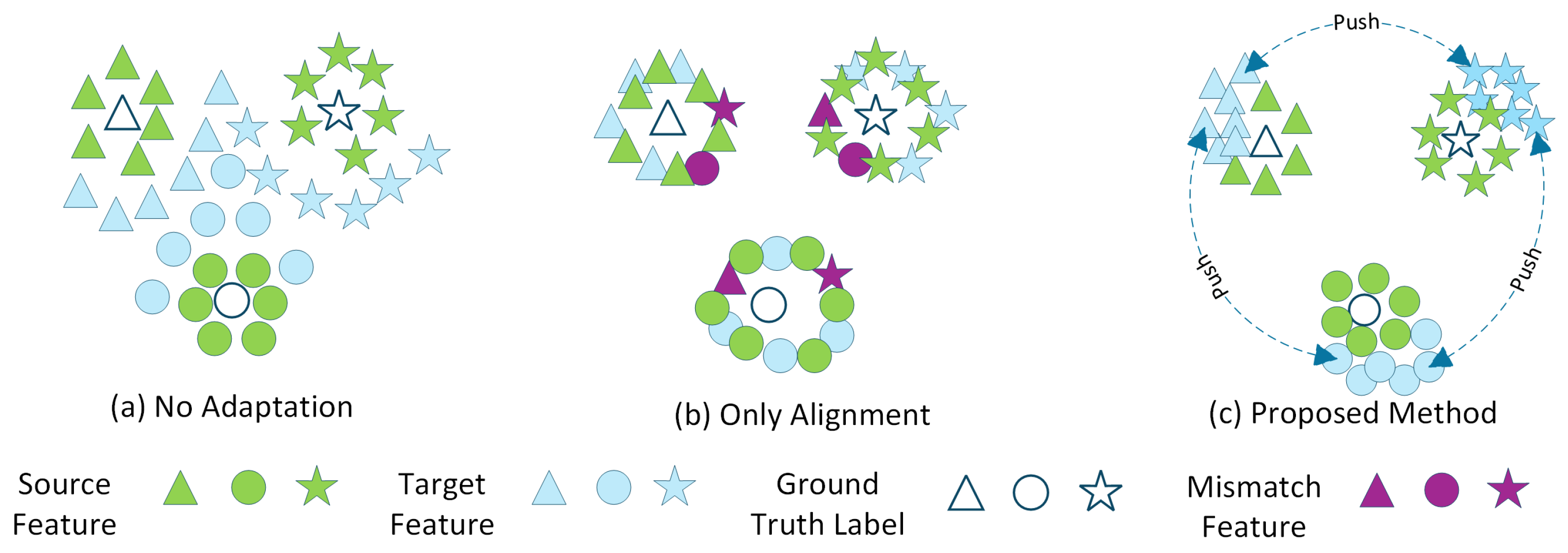Conditional Domain Adversarial Networks (CDAN) [6], for instance, employ a conditional domain discriminator and a multilinear conditioning strategy to adversarially train the feature extractor, thereby encouraging domain-invariant feature learning. Despite their effectiveness, existing approaches—irrespective of their methodological paradigm—generally assume that the learned feature space inherently exhibits a semantically meaningful structure that can be directly aligned across domains. In practice, however, global feature alignment may induce class-level mismatches, as illustrated in Figure 1b, where features from different classes remain entangled across domains. Consequently, samples belonging to different categories may become mixed in the latent space, leading to degraded classification performance.

In this work, we propose a contrastive domain adaptation framework that enhances class-level feature alignment for multi-sensor activity recognition. Motivated by the success of contrastive learning in self-supervised time-series representation learning [7], we design a structured sample grouping strategy that incorporates original samples together with carefully constructed positive and negative counterparts through augmentation and disturbance. Specifically, augmented samples that share the same class label are regarded as positive samples, whereas samples associated with different labels are treated as negative samples. For positive samples, we perform frequency-domain augmentation by transforming the signals using the Fourier transform and injecting Gaussian noise with a controlled magnitude, followed by an inverse Fourier transform to reconstruct the augmented signals in the temporal domain. For negative samples, since class labels in the target domain are unavailable, there exists an inherent risk of inadvertently selecting samples belonging to the same class as the anchor. To mitigate this issue, we introduce random disturbances to the selected negative samples by partially replacing segments of the original signal with synthetic perturbations. These disturbances are categorized into four types—local, global, trend and seasonal perturbations—thereby increasing the likelihood of semantic discrepancy between negative sample and the anchor. After constructing the sample groups, a contrastive loss is employed to promote class-consistent feature alignment while preserving inter-class separability [8]. By integrating this contrastive structure within an adversarial learning framework, the proposed method facilitates the learning of a feature space that is both domain-invariant and class-discriminative. Our contributions are summarized as follows:

• We introduce a contrastive discrimination paradigm integrated with adversarial learning for multi-sensor domain adaptation. The proposed framework incorporates a structured sample grouping strategy with contrastive loss constraints to enhance classification performance in the target domain.
• We propose an augmentation–disturbance strategy for constructing positive and negative samples. Specifically, Gaussian noise is injected into positive samples in the frequency domain, while negative samples are generated by partially perturbing the original signals with structured disturbances, thereby increasing semantic separability.
• We validate our approach on a real-world multi-sensor dataset, demonstrating superior performance compared to other UDA methods across different feature extractors.

2. Related Work

Domain adaptation for sensor-based human activity recognition (HAR) has attracted increasing attention due to distribution shifts caused by variations in subjects, sensor placement, environmental conditions, and device configurations. Existing approaches can generally be grouped into three methodological categories: discrepancy-driven, adversarial-learning-based, and reconstruction-oriented methods.

Discrepancy-driven approaches reduce cross-domain divergence by aligning statistical properties of feature representations extracted from multi-sensor signals. For example, HoMM [9] mitigates domain shift by matching higher-order moments of feature distributions, while DSAN [10] aligns subdomain-level statistics to reduce fine-grained discrepancies. Such strategies aim to enforce feature consistency across domains, which is particularly important in HAR scenarios where motion patterns vary significantly across individuals. Adversarial-learning-based methods introduce domain discriminators to encourage sensor features from different domains to become indistinguishable. DANN [11] employs a gradient reversal layer to guide the feature extractor toward domain-invariant representations, whereas DIRT [12] further enhances invariance through iterative adversarial refinement. CDAN [6] extends this paradigm by conditioning the discriminator on classifier outputs, facilitating multimodal alignment. In HAR settings, these methods help alleviate distribution mismatch induced by heterogeneous sensor characteristics and subject-dependent motion variability. Reconstruction-oriented approaches assume that reconstructing input signals can preserve domain-specific structure while promoting shared representations. SDA [13], for instance, learns unified representations capable of reconstructing data from multiple domains using a shared network. Although originally proposed for visual tasks, such strategies have been adapted to sequential sensor data to maintain temporal coherence.

Despite these advances, many existing methods are either originally designed for image-based applications or do not fully exploit the intrinsic properties of multi-sensor time-series signals, such as temporal continuity and cross-sensor correlation. To address time-series-specific challenges, several dedicated approaches have been proposed. AdvSKM [14] employs a kernel-based metric to quantify domain discrepancy in sequential representations. CoDATS [15] aligns temporal feature distributions through adversarial training with temporal consistency constraints. CoTMix [16] introduces contrastive learning with sequence-level mixup to generate synthetic time-series samples. However, when domain gaps are substantial, mixed sequences may deviate from realistic motion dynamics, limiting their effectiveness in HAR scenarios.

Motivated by these limitations, we develop a unified framework that integrates adversarial learning with a structured contrastive grouping mechanism tailored for multi-sensor sequential data. By explicitly enhancing class-level alignment while preserving temporal and semantic structure, the proposed approach facilitates the learning of discriminative and domain-robust representations for sensor-based HAR.

3. Problem Definition

We denote a multi-sensor dataset as $\mathcal{D}={\left\{(x_i,y_i)\right\}}_{i=1}^n$, where n is the number of multivariate time-series samples. Each sample $x_i\in {\mathbb{R}}^{T\times d}$ consists of readouts from d sensors over T time steps, while $y_i\in \{1,2,\dots ,N\}$ represents the corresponding label, where N denotes the number of classes, denoted as $\mathcal{C}$. Therefore, we define the labeled source domain dataset as ${\mathcal{D}}_s={\left\{(x_i^s,y_i^s)\right\}}_{i=1}^{n_s}$, where $n_s$ refer to the number of the source domain samples, $x_i^s$ represents the i-th source domain sample, and $y_i^s$ denotes the associated label. The target domain dataset is unlabeled and is denoted as ${\mathcal{D}}_t={\left\{\left(x_i^t\right)\right\}}_{i=1}^{n_t}$, where $n_t$ represents the number of unlabeled target domain samples. Source and target domains have samples drawn from source and target distributions, ${\mathcal{D}}_s\sim p_s(x^s,y^s)$ and ${\mathcal{D}}_t\sim p_t(x^t,y^t)$. Considering the assumption of the domain shift problem, we focus on the scenario where the marginal probability distributions of x differ, $p_s\left(x\right)\ne p_t\left(x\right)$, while conditional probability distributions remain constant across domains, $p_s\left(y\right|x)=p_t\left(y\right|x)$. However, when class-conditional distributions vary significantly between domains, domain alignment may result in suboptimal or biased decision boundaries. Such violations correspond to conditional shift and can lead to performance degradation. Accordingly, we adopt a model $h_{\theta }=g_{\theta }\circ f_{\theta }$, parameterized by $\theta$, where $f_{\theta }:\mathcal{X}\to \mathcal{Z}$ is a feature extractor mapping input data to a latent space $\mathcal{Z}$, and $g_{\theta }:\mathcal{Z}\to \mathcal{C}$ is a classifier mapping features to class predictions.

Following the domain adaptation theory in [17], let $\mathcal{H}$ be the hypothesis space and let $({\mathcal{D}}_s,{ϵ}_s)$ and $({\mathcal{D}}_t,{ϵ}_t)$ represent the two domains and their corresponding generalization error functions. Then for any $h\in \mathcal{H}$, we have the following inequality:

$${ϵ}_t\left(h\right)\le {ϵ}_s\left(h\right)+{\displaystyle \frac{1}{2}}{d}_{\mathcal{H}\Delta \mathcal{H}}({\mathcal{D}}_s,{\mathcal{D}}_t)+\lambda$$

(1)

where $\lambda ={min}_{h^{\prime }\in \mathcal{H}}[{ϵ}_t\left(h^{\prime }\right)+{ϵ}_s\left(h^{\prime }\right)]$, and $d_{\mathcal{H}\Delta \mathcal{H}}$ denotes the $\mathcal{H}\Delta \mathcal{H}$-distance between two domains, and is defined as

$$d_{\mathcal{H}\Delta \mathcal{H}}=2\underset{h,h^{\prime }\in \mathcal{H}}{sup}\mid {\mathbb{P}}_{{\mathcal{D}}_s}[h\ne h^{\prime }]-{\mathbb{P}}_{{\mathcal{D}}_t}[h\ne h^{\prime }]\mid$$

(2)

This bound reveals that the target error depends on three terms: the source error ${ϵ}_s\left(h\right)$, the divergence $\mathcal{H}\Delta \mathcal{H}$ between domains, and the joint optimal error of the ideal hypothesis across both domains. Thus, an effective UDA strategy aims to minimize the domain divergence while maintaining low source error, implicitly encouraging the learned hypothesis h to approach the optimal joint hypothesis $h^{\prime }$.

4. Methodology

4.1. Model Overview

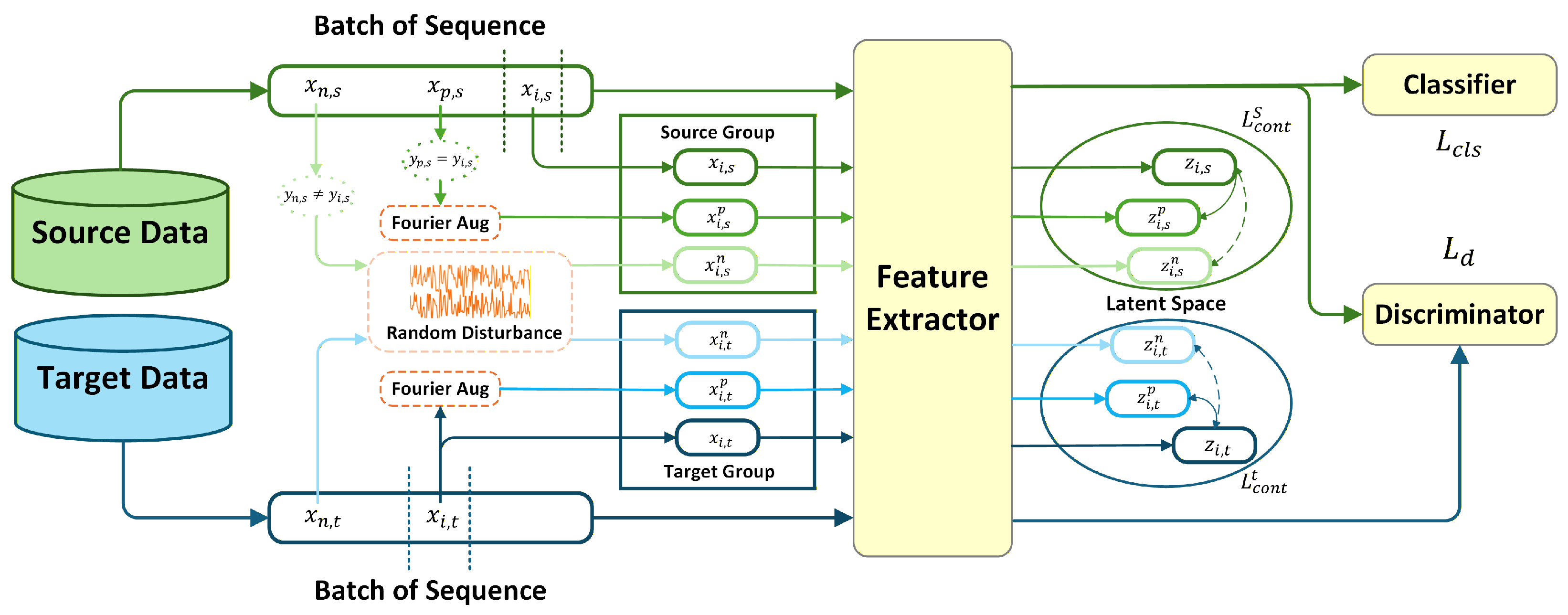
We tackle unsupervised domain adaptation (UDA) for human activity recognition in multi-sensor by enhancing the feature extractor with a tailored contrastive learning objective, as illustrated in Figure 2. Specifically, we introduce class-aware augmentation-disturbance strategy to construct positive and negative pair in the source domain and the target domain. By jointly minimizing the contrastive losses in both domains within an adversarial learning framework, our approach effectively reduces the divergence $\mathcal{H}\Delta \mathcal{H}$ between domains while promoting class-discriminative and domain-invariant feature representations.

4.2. Augmentation–Disturbance-Based Sample Grouping Strategy

For each anchor sample derived from multi-sensor sequential data, a corresponding group of positive and negative samples is constructed to form contrastive sample groups. In the source domain, where class labels are available, a sample sharing the same label as the anchor $x_{i,s}$ is selected as the positive sample $x_{p,s}$, while samples belonging to different classes are selected as negative samples $x_{n,s}$. In the target domain, where labels are unavailable, the anchor $x_{i,t}$ itself is used to construct the positive sample through augmentation, whereas another sequence is randomly selected from the same batch and treated as the negative sample $x_{n,t}$.

Contrastive learning relies on data augmentation to shape invariant feature representations, enforcing proximity among augmented views of the same signal and separation from representations of other signals [18]. Accordingly, augmentation is applied to construct positive pairs $x_i^p$. However, when negative samples are randomly selected from a batch, there exists an inherent risk that they may share the same underlying class as the anchor. 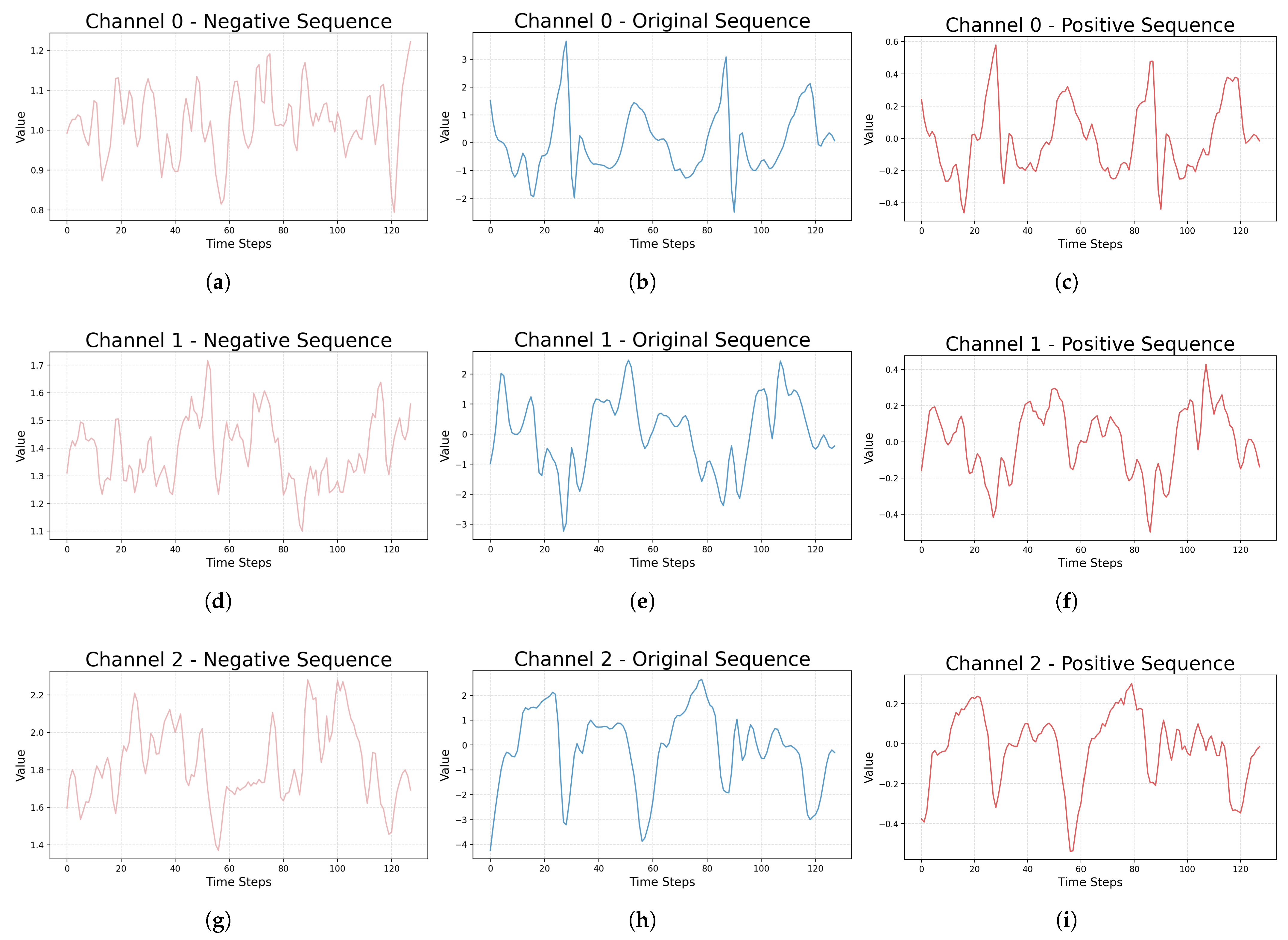To mitigate this issue, structured disturbances are introduced to construct negative pairs $x_i^n$, thereby increasing semantic discrepancy between contrastive pairs. The augmentation and perturbation strategies are described in detail in the following paragraphs, and an example of the constructed sample group is illustrated in Figure 3.

To construct positive pairs, we inject controlled noise into the original signals, as this directly enforces the inductive bias that the core semantic representation of a sample should remain invariant under continuous, low-magnitude perturbations in the input space. Such perturbations encourage a more robust and smoothly varying latent embedding. Specifically, we perform frequency-domain augmentation by injecting Gaussian noise into the Fourier spectrum of each sequence sample $x_i$ [19]. The procedure is defined as

$$\overline{x_i}=\Re \{{\mathcal{F}}^{-1}(\mathcal{F}\left\{x_i\right\}+\eta ·{\displaystyle \frac{1}{N}}\sum _{m=0}^{N-1}|X\left[m\right]|·({\mathcal{N}}_R\left[k\right]+j{\mathcal{N}}_I\left[k\right])\left)\right\}$$

(3)

where $X\left[m\right]$ is denoted as Discrete Fourier Transform of $x_i$:

$$X\left[m\right]=\mathcal{F}\left\{x_i\right\}\left[m\right]=\sum _{n=0}^{N-1}{x}_i\left[n\right]e^{-j2\pi mn/N},\hspace{1em}m,k\in \{0,1,\dots ,N-1\}$$

(4)

Here, $\mathcal{F}(·)$ and ${\mathcal{F}}^{-1}(·)$ denote the Fourier transform and its inverse, respectively, and $\Re \{·\}$ extracts the real part of the reconstructed signal. The parameter $\eta$ controls the noise magnitude. The terms ${\mathcal{N}}_R\left[k\right]$ and ${\mathcal{N}}_I\left[k\right]$ represent independent and identically distributed Gaussian noise applied to the real and imaginary components, respectively.

To construct negative pairs, a structured disturbance strategy is introduced to mitigate the risk of selecting samples that share the same underlying class as the anchor. Considering the intrinsic properties of multi-sensor sequential signals, the proposed disturbances are designed to reflect plausible variations observed in real-world sensor measurements rather than arbitrary noise injection. In practical HAR scenarios, sensor readings may exhibit localized abnormal spikes due to transient motion artifacts, sensor displacement, or environmental interference, as well as sustained temporal deviations caused by gradual posture changes or motion pattern shifts. Accordingly, we introduce two categories of perturbations. Point-level disturbances simulate instantaneous measurement anomalies by modifying individual timestamps using statistically extreme values derived from the signal distribution. Subsequence-level disturbances emulate structured temporal deviations, such as trend shifts or periodic pattern alterations, within a contiguous segment [20]. These perturbations preserve the overall signal structure while introducing sufficient semantic deviation, thereby ensuring that negative samples remain physically plausible yet discriminatively distinct from the anchor and positive samples. The disturbance ratio is varied from 5 data points to 90% of the entire sequence. For point-level disturbances, statistical properties of the signal are exploited to generate abnormal perturbations. Specifically, for the global disturbance, the mean ${\mu }_w$ and standard deviation ${\sigma }_w$ are computed over the entire sequence. Abnormal values are then randomly sampled from the group $\{{\mu }_w+m·{\sigma }_w,{\mu }_w-m·{\sigma }_w\}$, where $m\in [3, 5]$, and used to replace randomly selected points in the original signal. For the local disturbance, a local temporal region is first selected, within which the mean ${\mu }_l$ and standard deviation ${\sigma }_l$ are computed. Abnormal values sampled from group $\{{\mu }_l+m·{\sigma }_l,{\mu }_l-m·{\sigma }_l\}$ are then used to perturb randomly selected points within this region. For subsequence-level disturbances, a temporal segment is selected with start and end indices denoted by $p_1$ and $p_2$, respectively. The trend disturbance is defined as:

$$s^{\prime }\left(t\right)=\left\{\begin{array}{cc}s\left(t\right)+m{\sigma }_w\hfill & p_1\le t\le p_2\hfill \\ s\left(t\right)\hfill & \mathrm{Otherwise}.\hfill \end{array}\right.$$

(5)

where $s\left(t\right)$ and $s^{\prime }\left(t\right)$ denote the original and perturbed signals, respectively. In addition, the seasonal disturbance is defined as

$$s^{\prime }\left(t\right)=\left\{\begin{array}{cc}s(p_1+([t-p_1]·f)\hspace{1em}mod L)\hfill & p_1\le t<p_2,f\ne 1\hfill \\ s\left(t\right)\hfill & \mathrm{Otherwise}.\hfill \end{array}\right.$$

(6)

where f is a randomly sampled scaling factor and $L=p_2-p_1$ denotes the length of the disturbed subsequence.

4.3. Contrastive Discrimination Based on Adversarial Representation Learning

In our framework, the choice of feature extractor is flexible, as the focus lies in improving cross-domain feature alignment rather than evaluating extractor performance. For each domain, we obtain features for anchors and their corresponding positive negative samples: $z_{i,s},z_{i,s}^p,z_{i,s}^n\in {\mathcal{Z}}_s$ and $z_{i,t},z_{i,t}^p,z_{i,t}^n\in {\mathcal{Z}}_t$, where ${\mathcal{Z}}_s$ and ${\mathcal{Z}}_t$ representing source and target features, respectively. In the source domain, labeled data allow explicit construction of positive and negative pairs. This yields the following supervised contrastive loss:

$$\begin{array}{c}\hfill {\mathcal{L}}_{cont}^s={\displaystyle \frac{1}{\left|B\right|}}\sum _{i=1}^{\left|B\right|}max({\displaystyle \frac{1}{\left|N\right|}}\sum _{j=1}^{\left|N\right|}(\parallel z_{i,s}-z_{i,s}^p{\parallel }_2^2-\parallel z_{i,s}-z_{j,s}^n{\parallel }_2^2+m),0)\end{array}$$

(7)

where $\left|B\right|$ is the batch size, and $\left|N\right|$ is the number of negative samples in the batch. This loss function uses true source domain labels to enhance the separation of different class feature by at least the margin m. Compared with probability-based objectives such as InfoNCE, the Euclidean margin loss provides a clearer geometric interpretation, directly encouraging compact intra-class clustering and explicit inter-class separation. Moreover, it is easier to optimize and less sensitive to batch size. By leveraging explicit labels, this loss enforces clear inter-class separation in the source feature space. Importantly, this structured feature space also serves as a reference for aligning the target domain, implicitly guiding the learning of domain-invariant representations. In the target domain, where labels are unavailable, we rely on the assumption that nearby samples are more likely to share semantics. We construct pseudo-positive pairs using nearest neighbors and negatives using distant samples. The target unsupervised contrastive loss is

$$\begin{array}{c}\hfill {\mathcal{L}}_{cont}^t={\displaystyle \frac{1}{\left|B\right|}}\sum _{i=1}^{\left|B\right|}max(\parallel z_{i,t}-z_{i,t}^p{\parallel }_2^2-\parallel z_{i,t}-z_{i,t}^n{\parallel }_2^2+m,0)\end{array}$$

(8)

This enforces that target features are more tightly aligned with their positives while being separated from negatives, implicitly improving domain alignment and class- level discrimination.

To further mitigate domain shift, we incorporate an adversarial learning framework, which encourages the extraction of domain-invariant features. This framework includes a domain discriminator and a task classifier. The discriminator is trained to distinguish between source and target domain representations, while a Gradient Reversal Layer (GRL) allows adversarial signals to update the feature extractor by reversing gradients during backpropagation. The discriminator loss is defined as

$${\mathcal{L}}_d=\underset{D}{sup}[{\mathbb{E}}_{z\sim {\mathcal{Z}}_s}[lnD\left(z\right)]+{\mathbb{E}}_{z\sim {\mathcal{Z}}_t}[1-lnD\left(z\right)]]$$

(9)

In parallel, a task classifier minimizes the supervised classification loss on the source domain:

$${\mathcal{L}}_{cls}={\mathbb{E}}_{x,y\sim {\mathcal{D}}_s}[y\top ln{h}_{\theta }\left(x\right)]$$

(10)

which directly reduces the source error term ${ϵ}_s\left(h\right)$ in the theoretical domain adaptation bound based on $\mathcal{H}\Delta \mathcal{H}$-divergence. The overall training objective integrates all components as

$${\mathcal{L}}_{overall}=\alpha ·{\mathcal{L}}_{cont}^s+\beta ·{\mathcal{L}}_{cont}^t+\gamma ·{\mathcal{L}}_d+\lambda ·{\mathcal{L}}_{cls}$$

(11)

where hyperparameters $\alpha$, $\beta$, $\gamma$, $\lambda$ balance the contribution of each loss term. By jointly optimizing this objective, the model learns features that are discriminative, domain-invariant, and robust across source and target domains.

5. Experiments

5.1. Dataset

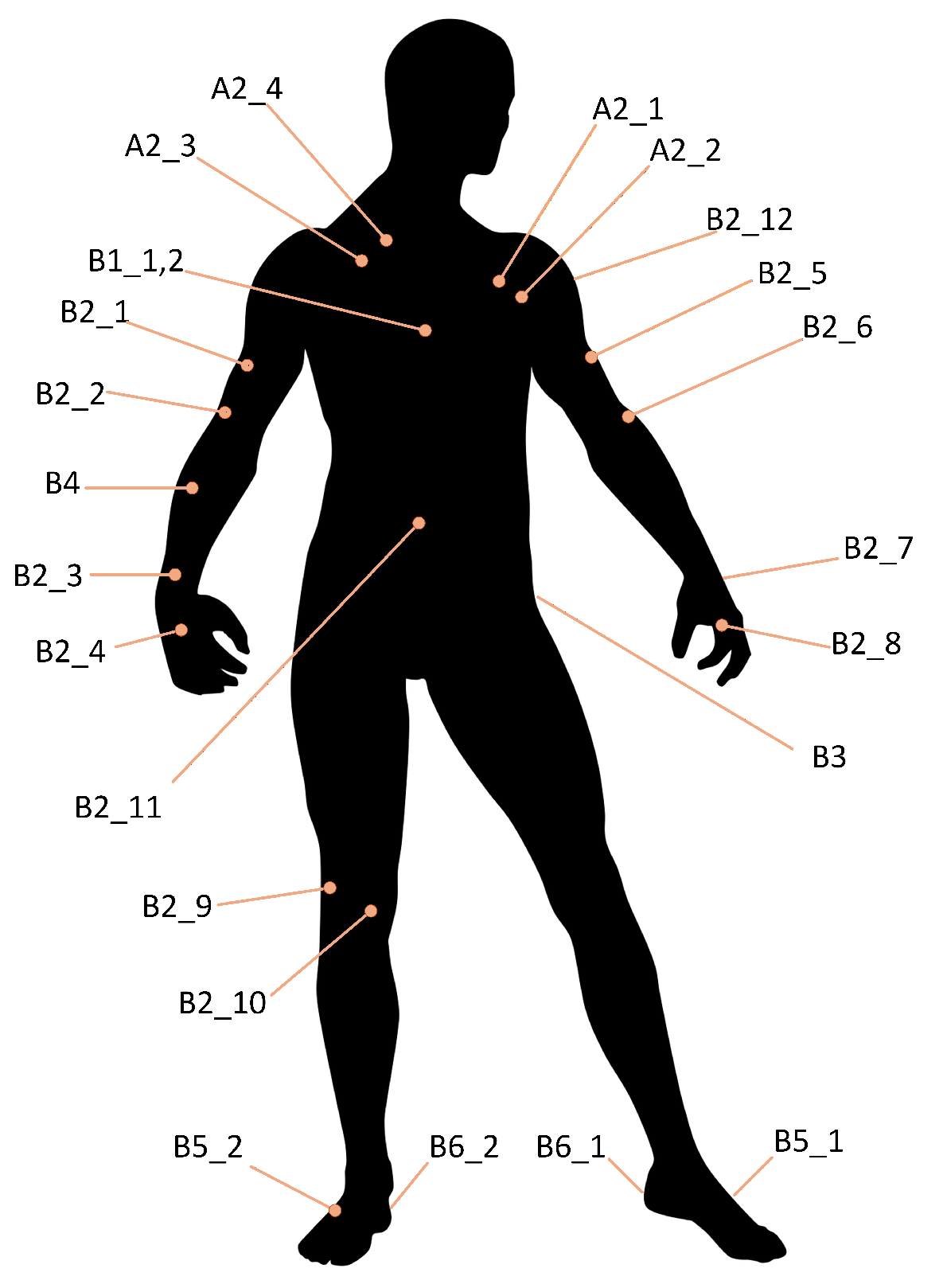
We select the publicly available Opportunity [21] dataset to evaluate our proposed method. This dataset includes a rich set of sensor modalities, such as inertial measurement units (IMUs), various body-worn sensors, and object-mounted sensors. The configuration of the body-worn sensors is illustrated in Figure 4. It provides extensive recordings of multiple subjects performing a wide range of activities, such as walking, sitting, and interacting with various objects. These characteristics make Opportunity particularly suitable for our study, as it enables rigorous evaluation under diverse motion patterns and sensor configurations. Furthermore, it is widely recognized as a benchmark in Human Activity Recognition (HAR) and sensor-based motion analysis, ensuring comparability with prior work and relevance to real-world applications.

5.2. Experimental Setup

We select baseline methods according to three criteria: (1) coverage of diverse unsupervised domain adaptation (UDA) paradigms, including adversarial approaches (e.g., CDAN [6]), discrepancy-based methods (e.g., DeepCORAL [4]), and reconstruction-based techniques (e.g., CoTMix [16]), enabling a comprehensive evaluation; (2) relevance to time-series domain adaptation, with a focus on methods designed for or adaptable to sequential data; and (3) inclusion of strong and widely recognized baselines to ensure a rigorous comparison. Each dataset is partitioned by subject into 70% training and 30% testing sets. All splits are normalized using statistics computed from the training data. Experiments are conducted on a server equipped with eight AMD EPYC 7702 64-core CPUs and an NVIDIA GeForce RTX 4090 GPU.

To effectively capture complex dependencies in multivariate sensor data, we adopt a Graph Neural Network (GNN) as the primary feature extractor. The architecture consists of three convolutional blocks augmented with Graph Convolutional Network (GCN) layers [22], enabling explicit modeling of spatial relationships among sensors. We first compare our proposed method with five representative baselines using the same GNN backbone to ensure a fair evaluation. Subsequently, we further analyze classification performance under different adaptation scenarios to validate the effectiveness of our approach. In the ablation study, we evaluate the robustness of our framework from three aspects. First, to verify that the method is not overly dependent on a specific backbone, we replace the GNN with a Temporal Convolutional Network (TCN). Second, we assess the individual contributions of each loss component under different adaptation settings. Third, we examine the necessity of the proposed augmentation–perturbation strategy on three different tasks. Finally, we conduct a sensitivity analysis to examine the influence of three key hyperparameters, along with a computational analysis to evaluate the actual computational cost of the proposed method.

For fair comparison, we standardize the training protocol, feature extractor configurations, and optimizer settings across all methods, following the AdaTime benchmark [23]. All models are trained for 40 epochs with a batch size of 32 using the Adam optimizer with a learning rate of $1\times {10}^{-3}$. Reported results are presented as the mean and standard deviation over 10 independent runs with different random seeds across five domain adaptation scenarios.

5.3. Experimental Performance

5.3.1. Comparison with Baselines

All methods are implemented using a unified architecture consisting of a representative GNN feature extractor followed by a single fully connected classification layer. This consistent design ensures a fair comparison by isolating the contribution of domain adaptation strategies. GNNs are particularly suitable for modeling spatial relationships among multiple sensors. Performance is evaluated using Accuracy and Macro-F1 (MF1). While Accuracy reflects overall correctness, MF1 provides a balanced evaluation under class-imbalanced conditions, which are common in human activity recognition datasets.

Table 1 reports the performance comparison on the Opportunity dataset. Statistical significance is assessed using a t-test, with p-values below 0.05 and 0.01 indicated in the table. The proposed method consistently achieves the best results, reaching 88.22% Accuracy and 85.95% MF1, demonstrating strong effectiveness and generalization capability. In contrast, CoTMix, a reconstruction-based approach that performs sequence-level mixup between domains, exhibits performance degradation. This is likely due to semantic distortion caused by mixing heterogeneous sequences, particularly in the unlabeled target domain.

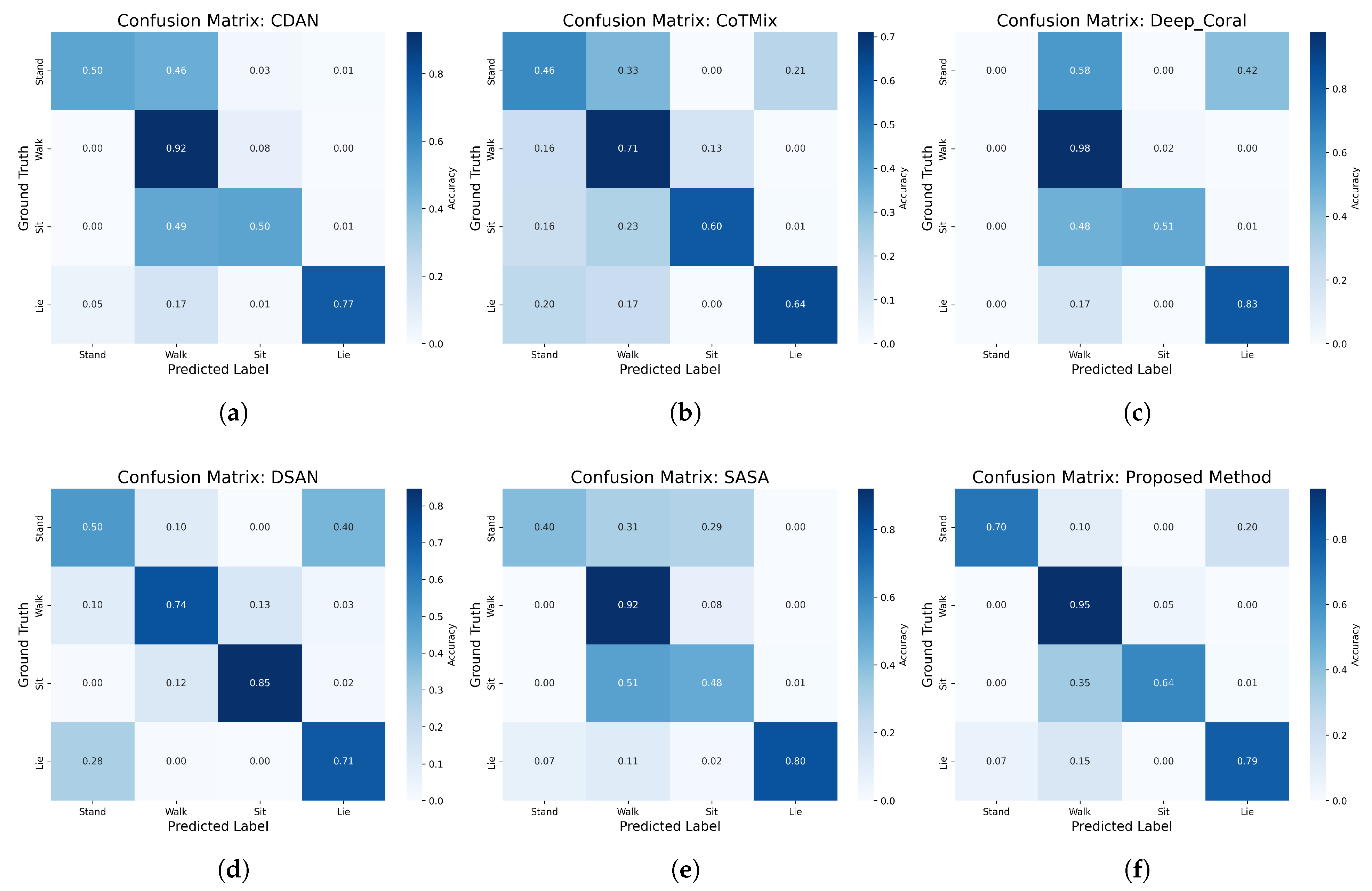
To further analyze baseline performance, we conduct class-wise evaluation. Table 2 presents overall target-domain accuracy, and Figure 5 illustrates the confusion matrix for the adaptation scenario from scenario 3 to scenario 1. Our method demonstrates superior stability and robustness across tasks, notably improving the classification of standing activity from walk and lie.

Although our experiments primarily focus on the Opportunity [21] dataset, as the augmentation and perturbation strategies are closely related to its sensor characteristics, we further evaluate our approach on the HHAR [24] dataset, another widely used benchmark for human activity recognition. As shown in Table 3, our method still outperforms the compared approaches overall, demonstrating its robustness and confirming that constructing high-quality negative samples is crucial for improving domain adaptation performance.

Table 1. Overall Accuracy and Macro-F1 (MF1) obtained by different unsupervised domain adaptation approaches on the Opportunity [21] dataset with a GNN-based feature extractor. The highest values in each column are shown in bold, and the second-highest values are underlined. Statistical significance is indicated by † (p < 0.05) and ‡ (p < 0.01).

GNN	CDAN [6]		CoTMix [16]		DeepCORAL [4]		DSAN [10]		SASA [25]		Ours
	Accuracy	Macro-F1 (MF1)	Accuracy	Macro-F1 (MF1)	Accuracy	Macro-F1 (MF1)	Accuracy	Macro-F1 (MF1)	Accuracy	Macro-F1 (MF1)	Accuracy	Macro-F1 (MF1)
3 → 1	77.05% ± 4.11% †	68.86% ± 13.65%	65.45% ± 22.06% †	56.69% ± 20.91% †	78.55% ± 4.09%	58.42% ± 3.96% ‡	73.95% ± 7.37% †	65.59% ± 9.68% †	76.75% ± 5.25% †	65.75% ± 14.81%	82.65% ± 6.26%	78.59% ± 14.43%
2 → 3	74.55% ± 5.05% ‡	58.32% ± 5.99% ‡	62.80% ± 20.75% †	59.04% ± 21.66%	79.65% ± 1.72%	60.41% ± 5.99% ‡	70.05% ± 5.10% ‡	53.05% ± 3.74% ‡	74.80% ± 4.23% ‡	58.81% ± 9.38% ‡	80.90% ± 3.07%	73.72% ± 3.58%
3 → 4	90.90% ± 2.14%	91.16% ± 1.87%	72.45% ± 23.32% †	65.28% ± 23.26% ‡	87.20% ± 2.99% ‡	69.86% ± 10.67% ‡	78.95% ± 5.16% ‡	72.20% ± 10.87% ‡	92.35% ± 2.36%	90.19% ± 9.14%	92.40% ± 0.94%	92.39% ± 1.06%
4 → 1	91.00% ± 1.63% †	91.74% ± 1.52% †	63.80% ± 21.29% ‡	57.39% ± 20.33% ‡	84.65% ± 3.23% ‡	84.78% ± 3.49% ‡	87.30% ± 4.24%	84.54% ± 6.48% †	89.50% ± 2.95%	90.91% ± 2.75%	88.80% ± 2.20%	89.60% ± 2.16%
1 → 3	84.75% ± 4.27% ‡	70.23% ± 13.58% ‡	72.35% ± 8.90% ‡	66.47% ± 11.63% ‡	77.70% ± 1.16% ‡	51.04% ± 2.81% ‡	73.70% ± 6.17% ‡	61.35% ± 11.09% ‡	80.85% ± 2.46% ‡	63.78% ± 8.03% ‡	90.25% ± 3.65%	87.34% ± 8.32%
2 → 4	88.55% ± 2.84% †	88.33% ± 4.54%	71.20% ± 22.84% †	68.18% ± 23.46% †	91.60% ± 1.60%	90.59% ± 2.51%	74.90% ± 6.43% ‡	60.99% ± 16.55% ‡	87.05% ± 2.29% ‡	86.08% ± 3.99% ‡	91.50% ± 1.78%	91.49% ± 1.38%
1 → 4	90.05% ± 2.29% ‡	87.72% ± 8.37%	79.20% ± 5.73% ‡	72.74% ± 6.56% ‡	83.15% ± 3.50% ‡	69.87% ± 11.55% ‡	75.70% ± 5.49% ‡	64.42% ± 16.45% ‡	89.80% ± 0.86% ‡	88.55% ± 2.70% ‡	93.55% ± 1.91%	92.86% ± 2.32%
3 → 2	73.60% ± 2.67%	59.07% ± 5.87%	65.90% ± 5.09% ‡	56.85% ± 5.88% †	80.50% ± 2.00% †	61.30% ± 1.51%	73.35% ± 9.72%	66.39% ± 11.17%	77.25% ± 4.35%	66.11% ± 10.39%	76.60% ± 5.08%	68.26% ± 13.53%
4 → 3	93.50% ± 0.85% ‡	92.86% ± 1.05% ‡	67.85% ± 32.01% †	64.84% ± 33.04% †	84.80% ± 2.10% ‡	71.26% ± 7.23% ‡	77.45% ± 8.03% ‡	66.76% ± 19.43% ‡	88.45% ± 3.83% †	83.41% ± 12.15%	91.65% ± 1.27%	90.84% ± 1.39%
2 → 1	93.65% ± 1.60%	94.22% ± 1.33%	68.70% ± 22.50% ‡	64.53% ± 22.10% ‡	88.65% ± 1.76% ‡	88.52% ± 2.14% ‡	86.65% ± 5.50% ‡	86.02% ± 7.63% ‡	92.70% ± 1.69%	93.28% ± 1.69%	93.85% ± 0.75%	94.39% ± 0.76%
Overall	85.76% ± 8.01% †	80.25% ± 15.48% ‡	68.97% ± 19.89% ‡	63.20% ± 20.23% ‡	83.64% ± 5.03% ‡	70.60% ± 14.18% ‡	77.20% ± 8.24% ‡	68.13% ± 15.25% ‡	84.95% ± 7.24% ‡	78.69% ± 15.18% ‡	88.22% ± 6.49%	85.95% ± 10.95%

Table 1. Overall Accuracy and Macro-F1 (MF1) obtained by different unsupervised domain adaptation approaches on the Opportunity [21] dataset with a GNN-based feature extractor. The highest values in each column are shown in bold, and the second-highest values are underlined. Statistical significance is indicated by † (p < 0.05) and ‡ (p < 0.01).

GNN	CDAN [6]		CoTMix [16]		DeepCORAL [4]		DSAN [10]		SASA [25]		Ours
	Accuracy	Macro-F1 (MF1)	Accuracy	Macro-F1 (MF1)	Accuracy	Macro-F1 (MF1)	Accuracy	Macro-F1 (MF1)	Accuracy	Macro-F1 (MF1)	Accuracy	Macro-F1 (MF1)
3 → 1	77.05% ± 4.11% †	68.86% ± 13.65%	65.45% ± 22.06% †	56.69% ± 20.91% †	78.55% ± 4.09%	58.42% ± 3.96% ‡	73.95% ± 7.37% †	65.59% ± 9.68% †	76.75% ± 5.25% †	65.75% ± 14.81%	82.65% ± 6.26%	78.59% ± 14.43%
2 → 3	74.55% ± 5.05% ‡	58.32% ± 5.99% ‡	62.80% ± 20.75% †	59.04% ± 21.66%	79.65% ± 1.72%	60.41% ± 5.99% ‡	70.05% ± 5.10% ‡	53.05% ± 3.74% ‡	74.80% ± 4.23% ‡	58.81% ± 9.38% ‡	80.90% ± 3.07%	73.72% ± 3.58%
3 → 4	90.90% ± 2.14%	91.16% ± 1.87%	72.45% ± 23.32% †	65.28% ± 23.26% ‡	87.20% ± 2.99% ‡	69.86% ± 10.67% ‡	78.95% ± 5.16% ‡	72.20% ± 10.87% ‡	92.35% ± 2.36%	90.19% ± 9.14%	92.40% ± 0.94%	92.39% ± 1.06%
4 → 1	91.00% ± 1.63% †	91.74% ± 1.52% †	63.80% ± 21.29% ‡	57.39% ± 20.33% ‡	84.65% ± 3.23% ‡	84.78% ± 3.49% ‡	87.30% ± 4.24%	84.54% ± 6.48% †	89.50% ± 2.95%	90.91% ± 2.75%	88.80% ± 2.20%	89.60% ± 2.16%
1 → 3	84.75% ± 4.27% ‡	70.23% ± 13.58% ‡	72.35% ± 8.90% ‡	66.47% ± 11.63% ‡	77.70% ± 1.16% ‡	51.04% ± 2.81% ‡	73.70% ± 6.17% ‡	61.35% ± 11.09% ‡	80.85% ± 2.46% ‡	63.78% ± 8.03% ‡	90.25% ± 3.65%	87.34% ± 8.32%
2 → 4	88.55% ± 2.84% †	88.33% ± 4.54%	71.20% ± 22.84% †	68.18% ± 23.46% †	91.60% ± 1.60%	90.59% ± 2.51%	74.90% ± 6.43% ‡	60.99% ± 16.55% ‡	87.05% ± 2.29% ‡	86.08% ± 3.99% ‡	91.50% ± 1.78%	91.49% ± 1.38%
1 → 4	90.05% ± 2.29% ‡	87.72% ± 8.37%	79.20% ± 5.73% ‡	72.74% ± 6.56% ‡	83.15% ± 3.50% ‡	69.87% ± 11.55% ‡	75.70% ± 5.49% ‡	64.42% ± 16.45% ‡	89.80% ± 0.86% ‡	88.55% ± 2.70% ‡	93.55% ± 1.91%	92.86% ± 2.32%
3 → 2	73.60% ± 2.67%	59.07% ± 5.87%	65.90% ± 5.09% ‡	56.85% ± 5.88% †	80.50% ± 2.00% †	61.30% ± 1.51%	73.35% ± 9.72%	66.39% ± 11.17%	77.25% ± 4.35%	66.11% ± 10.39%	76.60% ± 5.08%	68.26% ± 13.53%
4 → 3	93.50% ± 0.85% ‡	92.86% ± 1.05% ‡	67.85% ± 32.01% †	64.84% ± 33.04% †	84.80% ± 2.10% ‡	71.26% ± 7.23% ‡	77.45% ± 8.03% ‡	66.76% ± 19.43% ‡	88.45% ± 3.83% †	83.41% ± 12.15%	91.65% ± 1.27%	90.84% ± 1.39%
2 → 1	93.65% ± 1.60%	94.22% ± 1.33%	68.70% ± 22.50% ‡	64.53% ± 22.10% ‡	88.65% ± 1.76% ‡	88.52% ± 2.14% ‡	86.65% ± 5.50% ‡	86.02% ± 7.63% ‡	92.70% ± 1.69%	93.28% ± 1.69%	93.85% ± 0.75%	94.39% ± 0.76%
Overall	85.76% ± 8.01% †	80.25% ± 15.48% ‡	68.97% ± 19.89% ‡	63.20% ± 20.23% ‡	83.64% ± 5.03% ‡	70.60% ± 14.18% ‡	77.20% ± 8.24% ‡	68.13% ± 15.25% ‡	84.95% ± 7.24% ‡	78.69% ± 15.18% ‡	88.22% ± 6.49%	85.95% ± 10.95%

Table 2. Class-wise classification accuracy of different methods across all evaluation scenarios. The highest values in each column are shown in bold, and the second-highest values are underlined.

	Stand	Walk	Sit	Lie
CDAN [6]	67.11%	92.91%	70.25%	92.52%
CoTMix [16]	71.19%	70.08%	67.54%	68.52%
DeepCORAL [4]	37.89%	97.03%	50.99%	94.86%
DSAN [10]	54.05%	76.40%	73.76%	91.74%
SASA [25]	60.89%	89.13%	75.35%	93.77%
Ours	82.44%	95.00%	69.78%	92.17%

Table 2. Class-wise classification accuracy of different methods across all evaluation scenarios. The highest values in each column are shown in bold, and the second-highest values are underlined.

	Stand	Walk	Sit	Lie
CDAN [6]	67.11%	92.91%	70.25%	92.52%
CoTMix [16]	71.19%	70.08%	67.54%	68.52%
DeepCORAL [4]	37.89%	97.03%	50.99%	94.86%
DSAN [10]	54.05%	76.40%	73.76%	91.74%
SASA [25]	60.89%	89.13%	75.35%	93.77%
Ours	82.44%	95.00%	69.78%	92.17%

Table 3. Overall Accuracy and Macro-F1 (MF1) obtained by different unsupervised domain adaptation approaches on the HHAR [24] dataset with a GNN-based feature extractor. The highest values in each column are shown in bold, and the second-highest values are underlined. Statistical significance is indicated by † (p < 0.05) and ‡ (p < 0.01).

GNN	CDAN [6]		CoTMix [16]		DeepCORAL [4]		DSAN [10]		SASA [25]		Ours
	Accuracy	Macro-F1 (MF1)	Accuracy	Macro-F1 (MF1)	Accuracy	Macro-F1 (MF1)	Accuracy	Macro-F1 (MF1)	Accuracy	Macro-F1 (MF1)	Accuracy	Macro-F1 (MF1)
0 → 6	52.51% ± 7.21%	50.28% ± 6.68%	65.67% ± 25.05%	57.22% ± 27.48%	60.44% ± 9.52%	54.20% ± 9.14%	55.35% ± 8.86%	53.50% ± 8.30%	58.78% ± 9.14%	54.91% ± 8.12%	54.89% ± 6.37%	50.85% ± 5.80%
1 → 6	92.96% ± 1.78%	92.92% ± 1.76%	47.16% ± 37.49% ‡	39.21% ± 44.07% ‡	83.89% ± 4.25% ‡	83.72% ± 4.84% ‡	93.39% ± 1.68%	93.38% ± 1.69%	91.64% ± 0.60%	91.59% ± 0.58%	92.25% ± 1.10%	92.19% ± 1.13%
2 → 7	59.94% ± 1.50% †	60.34% ± 1.08% †	79.02% ± 4.70% ‡	71.80% ± 5.08% ‡	48.14% ± 3.23% ‡	44.12% ± 2.95% ‡	58.00% ± 7.00%	56.94% ± 7.83%	51.31% ± 8.07%	48.37% ± 7.05% †	55.84% ± 3.93%	55.63% ± 4.78%
3 → 8	87.41% ± 9.03% †	87.40% ± 9.18% †	71.23% ± 35.33%	67.28% ± 42.61%	79.04% ± 1.38% ‡	78.48% ± 1.71% ‡	95.40% ± 0.90%	95.62% ± 0.90%	82.07% ± 5.49% ‡	81.70% ± 5.73% ‡	95.77% ± 0.94%	95.97% ± 0.93%
4 → 5	97.50% ± 0.41% ‡	97.58% ± 0.40% ‡	78.65% ± 30.51%	75.01% ± 36.93%	82.94% ± 6.38% ‡	83.19% ± 6.33% ‡	96.81% ± 0.61% ‡	96.89% ± 0.59% ‡	94.95% ± 2.08%	95.08% ± 2.17%	93.13% ± 3.21%	93.19% ± 3.27%
5 → 0	32.60% ± 9.89% ‡	30.18% ± 8.66% ‡	65.97% ± 16.40% †	60.80% ± 19.50%	39.78% ± 2.77% ‡	35.65% ± 3.81% ‡	27.42% ± 5.56% ‡	29.17% ± 4.95% ‡	33.15% ± 3.42% ‡	28.45% ± 3.27% ‡	50.41% ± 4.61%	48.56% ± 3.51%
6 → 1	94.31% ± 1.03% †	94.16% ± 1.09% †	87.67% ± 23.21%	86.08% ± 28.17%	85.06% ± 2.21% ‡	84.45% ± 2.35% ‡	95.36% ± 0.80% ‡	95.24% ± 0.84% ‡	93.04% ± 1.78%	92.89% ± 1.83%	93.13% ± 1.28%	93.00% ± 1.31%
7 → 4	96.39% ± 1.18% †	96.45% ± 1.11% †	93.21% ± 2.15%	93.20% ± 2.63%	87.34% ± 4.36% ‡	87.21% ± 4.34% ‡	96.41% ± 0.96% †	96.42% ± 0.92% †	92.00% ± 1.12%	91.84% ± 1.18%	93.69% ± 3.37%	93.71% ± 3.29%
8 → 3	93.77% ± 10.65%	94.11% ± 9.81%	64.38% ± 33.62% †	58.47% ± 38.36% †	76.13% ± 8.60% ‡	72.92% ± 11.22% ‡	96.83% ± 0.39% †	96.91% ± 0.38% †	96.85% ± 0.40% †	96.94% ± 0.40% †	95.69% ± 1.42%	95.78% ± 1.49%
0 → 2	77.41% ± 3.70%	70.80% ± 4.83%	72.47% ± 19.33%	64.87% ± 21.06%	66.59% ± 3.07% ‡	59.59% ± 4.16% ‡	73.45% ± 3.75%	67.92% ± 3.31%	77.43% ± 2.75%	70.21% ± 2.52%	76.42% ± 3.65%	69.61% ± 3.63%
Overall	78.48% ± 22.27%	77.42% ± 23.07%	72.54% ± 27.40% †	67.39% ± 32.13% ‡	70.94% ± 16.64% ‡	68.35% ± 18.63% ‡	78.84% ± 23.64%	78.20% ± 23.75%	77.12% ± 21.41%	75.20% ± 23.07%	80.12% ± 18.49%	78.85% ± 19.62%

Table 3. Overall Accuracy and Macro-F1 (MF1) obtained by different unsupervised domain adaptation approaches on the HHAR [24] dataset with a GNN-based feature extractor. The highest values in each column are shown in bold, and the second-highest values are underlined. Statistical significance is indicated by † (p < 0.05) and ‡ (p < 0.01).

GNN	CDAN [6]		CoTMix [16]		DeepCORAL [4]		DSAN [10]		SASA [25]		Ours
	Accuracy	Macro-F1 (MF1)	Accuracy	Macro-F1 (MF1)	Accuracy	Macro-F1 (MF1)	Accuracy	Macro-F1 (MF1)	Accuracy	Macro-F1 (MF1)	Accuracy	Macro-F1 (MF1)
0 → 6	52.51% ± 7.21%	50.28% ± 6.68%	65.67% ± 25.05%	57.22% ± 27.48%	60.44% ± 9.52%	54.20% ± 9.14%	55.35% ± 8.86%	53.50% ± 8.30%	58.78% ± 9.14%	54.91% ± 8.12%	54.89% ± 6.37%	50.85% ± 5.80%
1 → 6	92.96% ± 1.78%	92.92% ± 1.76%	47.16% ± 37.49% ‡	39.21% ± 44.07% ‡	83.89% ± 4.25% ‡	83.72% ± 4.84% ‡	93.39% ± 1.68%	93.38% ± 1.69%	91.64% ± 0.60%	91.59% ± 0.58%	92.25% ± 1.10%	92.19% ± 1.13%
2 → 7	59.94% ± 1.50% †	60.34% ± 1.08% †	79.02% ± 4.70% ‡	71.80% ± 5.08% ‡	48.14% ± 3.23% ‡	44.12% ± 2.95% ‡	58.00% ± 7.00%	56.94% ± 7.83%	51.31% ± 8.07%	48.37% ± 7.05% †	55.84% ± 3.93%	55.63% ± 4.78%
3 → 8	87.41% ± 9.03% †	87.40% ± 9.18% †	71.23% ± 35.33%	67.28% ± 42.61%	79.04% ± 1.38% ‡	78.48% ± 1.71% ‡	95.40% ± 0.90%	95.62% ± 0.90%	82.07% ± 5.49% ‡	81.70% ± 5.73% ‡	95.77% ± 0.94%	95.97% ± 0.93%
4 → 5	97.50% ± 0.41% ‡	97.58% ± 0.40% ‡	78.65% ± 30.51%	75.01% ± 36.93%	82.94% ± 6.38% ‡	83.19% ± 6.33% ‡	96.81% ± 0.61% ‡	96.89% ± 0.59% ‡	94.95% ± 2.08%	95.08% ± 2.17%	93.13% ± 3.21%	93.19% ± 3.27%
5 → 0	32.60% ± 9.89% ‡	30.18% ± 8.66% ‡	65.97% ± 16.40% †	60.80% ± 19.50%	39.78% ± 2.77% ‡	35.65% ± 3.81% ‡	27.42% ± 5.56% ‡	29.17% ± 4.95% ‡	33.15% ± 3.42% ‡	28.45% ± 3.27% ‡	50.41% ± 4.61%	48.56% ± 3.51%
6 → 1	94.31% ± 1.03% †	94.16% ± 1.09% †	87.67% ± 23.21%	86.08% ± 28.17%	85.06% ± 2.21% ‡	84.45% ± 2.35% ‡	95.36% ± 0.80% ‡	95.24% ± 0.84% ‡	93.04% ± 1.78%	92.89% ± 1.83%	93.13% ± 1.28%	93.00% ± 1.31%
7 → 4	96.39% ± 1.18% †	96.45% ± 1.11% †	93.21% ± 2.15%	93.20% ± 2.63%	87.34% ± 4.36% ‡	87.21% ± 4.34% ‡	96.41% ± 0.96% †	96.42% ± 0.92% †	92.00% ± 1.12%	91.84% ± 1.18%	93.69% ± 3.37%	93.71% ± 3.29%
8 → 3	93.77% ± 10.65%	94.11% ± 9.81%	64.38% ± 33.62% †	58.47% ± 38.36% †	76.13% ± 8.60% ‡	72.92% ± 11.22% ‡	96.83% ± 0.39% †	96.91% ± 0.38% †	96.85% ± 0.40% †	96.94% ± 0.40% †	95.69% ± 1.42%	95.78% ± 1.49%
0 → 2	77.41% ± 3.70%	70.80% ± 4.83%	72.47% ± 19.33%	64.87% ± 21.06%	66.59% ± 3.07% ‡	59.59% ± 4.16% ‡	73.45% ± 3.75%	67.92% ± 3.31%	77.43% ± 2.75%	70.21% ± 2.52%	76.42% ± 3.65%	69.61% ± 3.63%
Overall	78.48% ± 22.27%	77.42% ± 23.07%	72.54% ± 27.40% †	67.39% ± 32.13% ‡	70.94% ± 16.64% ‡	68.35% ± 18.63% ‡	78.84% ± 23.64%	78.20% ± 23.75%	77.12% ± 21.41%	75.20% ± 23.07%	80.12% ± 18.49%	78.85% ± 19.62%

5.3.2. Ablation Study

To verify that the proposed framework is not overly dependent on a specific backbone, we evaluate its robustness by replacing the primary GNN with a Temporal Convolutional Network (TCN) [23] as an alternative feature extractor. As summarized in

Table 4. Comparison of baseline methods on the Opportunity [21] dataset with a TCN-based feature extractor. The highest values in each column are shown in bold, and the second-highest values are underlined. Statistical significance is indicated by † (p < 0.05) and ‡ (p < 0.01).

TCN	CDAN [6]		CoTMix [16]		DeepCORAL [4]		DSAN [10]		SASA [25]		Ours
	Accuracy	Macro-F1 (MF1)	Accuracy	Macro-F1 (MF1)	Accuracy	Macro-F1 (MF1)	Accuracy	Macro-F1 (MF1)	Accuracy	Macro-F1 (MF1)	Accuracy	Macro-F1 (MF1)
2 → 3	80.05% ± 4.24%	64.47% ± 8.33% †	66.35% ± 5.94% ‡	60.24% ± 10.31% ‡	78.95% ± 1.42%	60.50% ± 2.85% ‡	70.55% ± 2.18% ‡	53.53% ± 1.65% ‡	73.60% ± 2.63% ‡	57.34% ± 4.02% ‡	80.90% ± 4.45%	74.19% ± 7.11%
3 → 4	90.90% ± 3.63%	88.64% ± 10.11%	82.05% ± 3.71% ‡	80.87% ± 5.18% ‡	90.30% ± 1.34% †	89.57% ± 2.58% †	75.80% ± 4.74% ‡	67.35% ± 10.36% ‡	92.45% ± 1.21% ‡	92.66% ± 1.16%	92.00% ± 1.53%	91.98% ± 1.56%
4 → 1	85.40% ± 3.75%	86.79% ± 2.84%	66.55% ± 2.89% ‡	63.03% ± 2.81% ‡	87.80% ± 2.10%	89.12% ± 1.94%	79.05% ± 3.79% ‡	79.82% ± 6.33% ‡	90.30% ± 2.70% ‡	91.38% ± 2.47% ‡	86.60% ± 2.44%	88.10% ± 2.20%
1 → 3	87.15% ± 4.49%	78.01% ± 14.26%	69.00% ± 7.77% ‡	64.54% ± 12.60% ‡	82.35% ± 2.42% ‡	61.83% ± 2.06% ‡	71.35% ± 1.11% ‡	53.70% ± 0.73% ‡	81.70% ± 3.01% ‡	62.27% ± 4.61% ‡	90.25% ± 4.20%	87.76% ± 9.88%
2 → 4	91.50% ± 3.26%	89.84% ± 9.58%	77.00% ± 7.04% ‡	75.24% ± 7.92% ‡	90.15% ± 1.62%	87.09% ± 3.91%	79.15% ± 2.93% ‡	77.94% ± 10.62% ‡	87.25% ± 2.72% ‡	87.23% ± 2.55% †	90.20% ± 1.16%	89.79% ± 1.81%
Overall	87.00% ± 5.62%	81.55% ± 13.39% †	72.19% ± 8.42% ‡	68.78% ± 11.41% ‡	85.91% ± 4.89% †	77.62% ± 13.86% ‡	75.18% ± 4.81% ‡	66.47% ± 13.39% ‡	85.06% ± 7.26% †	78.18% ± 15.64% ‡	87.99% ± 4.96%	86.36% ± 8.32%

, our method maintains strong performance even when transitioned to a purely temporal-based architecture. This consistency across different architectural paradigms demonstrates that the efficacy of our domain adaptation strategy is backbone-agnostic and generalizes well to diverse feature extraction mechanisms.

To evaluate the individual contributions of the components within our framework, we conduct a systematic ablation study on the loss functions. While the classification loss ${\mathcal{L}}_{cls}$ is retained across all variants, we analyze the impact of the source-domain contrastive loss ${\mathcal{L}}_{cont}^s$, a target-domain contrastive loss ${\mathcal{L}}_{cont}^t$ and and a domain discriminator loss ${\mathcal{L}}_d$.

The results in

Table 5. Ablation results evaluating the contributions of each loss components. The highest values in each row are shown in bold.

Loss Component			3 → 1		4 → 2
${\mathcal{L}}_{\mathbf{cont}}^{\mathbf{s}}$	${\mathcal{L}}_{\mathbf{cont}}^{\mathbf{t}}$	${\mathcal{L}}_{\mathbf{d}}$	Accuracy	Macro-F1	Accuracy	Macro-F1
/	•	•	80.00%	75.90%	82.05%	81.74%
•	/	•	80.60%	73.92%	83.10%	82.80%
•	•	/	82.10%	61.64%	83.45%	79.37%
/	/	•	79.10%	74.57%	83.10%	82.78%
•	•	•	82.65%	78.59%	83.75%	83.29%

“/” denotes absence of the component, while “•” denotes inclusion.

indicate that the removal of contrastive learning from either domain consistently leads to a deterioration in classification accuracy compared to the full configuration. Specifically, when contrastive learning is restricted to the target domain, features tend to cluster without sufficient semantic alignment. Conversely, applying it solely to the source domain forces target features to align rigidly with source-class centers, failing to capture the intrinsic structure within the target domain. Furthermore, the discriminator loss ${\mathcal{L}}_d$ proves crucial for promoting the aggregation of target features toward their respective semantic centers. These observations underscore the necessity of jointly leveraging dual-domain contrastive objectives and adversarial learning.

Finally, we evaluate the efficacy of our proposed data augmentation and perturbation grouping strategy. As shown in

Table 6. Ablation study results evaluating the efficiency of augmentation and perturbation strategies. The highest values in each row are shown in bold.

Augment Sample		3 → 1		2 → 4		2 → 3
Postive	Negative	Accuracy	MF1	Accuracy	MF1	Accuracy	MF1
/	/	78.35%	74.30%	91.35%	91.16%	78.15%	72.35%
$\mathcal{F}$	$\mathcal{F}$	81.50%	81.20%	91.15%	91.35%	78.10%	70.51%
$\mathcal{F}$	Ours	82.65%	78.59%	91.50%	91.49%	80.90%	73.72%

, the experimental results across three scenarios support the consensus in contrastive learning research that proper augmentation is essential for performance. We further compare our perturbation strategy for negative sample construction against standard Fourier augmentation ($\mathcal{F}$). We observe that since Fourier augmentation primarily adds frequency noise to sequences, it may result in negative samples that are insufficiently discriminative from positive samples, potentially leading to a slight performance drop compared to the no-augmentation baseline. In contrast, our perturbation strategy is specifically designed to enhance the discriminability of negative sequences relative to the anchor and positive samples, thereby facilitating the learning of more robust and separable representations.

5.3.3. Sensitivity and Computational Analysis

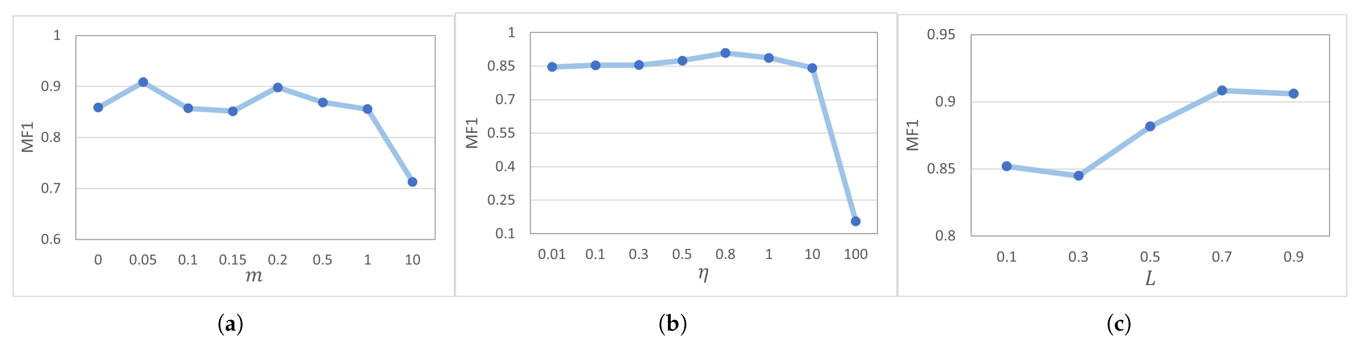
We conduct a sensitivity analysis on the Scenario 3 → Scenario 1 domain adaptation task to evaluate the impact of three key hyperparameters: the separation margin m, the Fourier-transform-based augmentation ratio $\eta$ and and the disturbance-affected area L. As illustrated in Figure 6, increasing the margin m helps establish clearer decision boundaries and does not lead to severe performance degradation even at larger values, indicating that the proposed method is relatively robust to this parameter. In contrast, the augmentation ratio $\eta$ exhibits a clear upper bound: excessively large values result in performance collapse, as positive samples become dominated by noise and lose their semantic consistency. Finally, the results show that increasing the disturbance-affected area L generally improves performance by encouraging tighter clustering of target-domain features, thereby enhancing final classification accuracy.

Table 7. Comparison of computational cost with baseline methods in terms of parameter count, training time, FLOPs, and inference latency for practical deployment.

	Parameters (M)	Training Time (s/epoch)	FLOPs (M)	Inference Time (ms)
CDAN [6]	1.22	0.63	74.31	0.4514
CoTMix [16]	0.62	0.83	144	0.4309
DeepCORAL [4]	0.62	0.67	82.51	0.4538
DSAN [10]	0.62	0.63	35.95	0.4348
SASA [6]	0.65	0.61	71.88	0.7472
Ours	1.09	3.17	218	0.4370

reports the computational cost of our method compared with several baselines. Our approach incurs a higher training time (3.17 s/epoch), mainly due to the CPU-based perturbation generation used to construct high-quality negative pairs. In addition, the feature extractor is repeatedly applied to learn representations from the augmented and perturbed samples, rather than processing a single source–target pair as in conventional methods. To further analyze the computational overhead, we compare our method with the adversarial-based approach CDAN [6] in

Table 8. Comparison with CDAN in terms of FLOPs consumption and parameter counts of each trainable component.

Methodology	Components	Parameters (M)	FLOPs (M)
CDAN [6]	Feature Extractor	0.612	71.882
	Discrminator	0.594	2.376
	Classifier	0.009	0.009
	Overall	1.216	74.314
Ours	Feature Extractor	0.612	216
	Projector	0.312	1.869
	Discrminator	0.152	0.303
	Classifier	0.009	0.009
	Overall	1.085	218

. The results show that the FLOPs of the feature extractor in our framework are approximately three times those of CDAN during training. However, this additional cost is strictly confined to the offline training phase. During inference, the feature extractor is executed only once, and the proposed method maintains a highly competitive inference latency (0.4370 ms), demonstrating its suitability for real-time deployment.

6. Limitation and Future Work

Although the experimental results demonstrate the effectiveness and robustness of the proposed framework, several limitations remain. A primary constraint lies in the construction of high-quality negative pairs, which is physics-informed and relies on the inherent physical properties and spatial correlations of sensor data. In this study, the perturbation strategy was tailored to the sensor configuration and semantic activity patterns of the Opportunity benchmark. While this design ensures physically meaningful negative samples, it requires manual adaptation when applied to datasets with substantially different sensor modalities or configurations.

Nevertheless, incorporating physical consistency into contrastive learning is essential for mitigating semantic misalignment in unsupervised domain adaptation. As future work, we plan to develop adaptive perturbation policies capable of automatically inferring physical constraints from sensor metadata, thereby improving generalization across diverse human activity recognition scenarios.

7. Conclusions

We propose a domain adaptation framework for multi-sensor human activity recognition that integrates a contrastive discrimination strategy within an adversarial learning architecture. Specifically, contrastive sample groups are constructed via an augmentation–disturbance mechanism and processed by a shared feature extractor, guided by a contrastive loss applied to both source and target domains. This design encourages semantically similar samples to cluster in the feature space while separating dissimilar ones, even in the absence of target-domain labels. Experiments conducted on the Opportunity dataset provide initial validation of the proposed framework. The results demonstrate consistent performance improvements over representative domain adaptation baselines, indicating that the proposed contrastive grouping strategy is effective in mitigating domain shifts in multi-sensor human activity recognition.

References

- Olugbade, T.; He, L.; Maiolino, P.; Heylen, D.; Bianchi-Berthouze, N. Touch Technology in Affective Human–, Robot–, and Virtual–Human Interactions: A Survey. Proc. IEEE 2023, 111, 1333–1354. [Google Scholar] [CrossRef]
- Meng, W.; Liu, Z.; Li, B.; Cui, W.; Zhou, J.T.; Zhang, L. GrapHAR: A Lightweight Human Activity Recognition Model by Exploring the Sub-Carrier Correlations. IEEE Trans. Wirel. Commun. 2024, 23, 2755–2770. [Google Scholar] [CrossRef]
- Wang, M.; Deng, W. Deep visual domain adaptation: A survey. Neurocomputing 2018, 312, 135–153. [Google Scholar] [CrossRef]
- Sun, B.; Saenko, K. Deep coral: Correlation alignment for deep domain adaptation. In Computer Vision—ECCV 2016 Workshops; Springer: Cham, Switzerland, 2016; pp. 443–450. [Google Scholar] [CrossRef]
- Goodfellow, I.J.; Pouget-Abadie, J.; Mirza, M.; Xu, B.; Warde-Farley, D.; Ozair, S.; Courville, A.; Bengio, Y. Generative adversarial nets. Adv. Neural Inf. Process. Syst. 2014, 27, 2672–2680. [Google Scholar]
- Long, M.; Cao, Z.; Wang, J.; Jordan, M.I. Conditional adversarial domain adaptation. Adv. Neural Inf. Process. Syst. 2018, 31, 1–11. [Google Scholar]
- Eldele, E.; Ragab, M.; Chen, Z.; Wu, M.; Kwoh, C.K.; Li, X.; Guan, C. Self-Supervised Contrastive Representation Learning for Semi-Supervised Time-Series Classification. IEEE Trans. Pattern Anal. Mach. Intell. 2023, 45, 15604–15618. [Google Scholar] [CrossRef] [PubMed]
- Darban, Z.Z.; Yang, Y.; Webb, G.I.; Aggarwal, C.C.; Wen, Q.; Pan, S.; Salehi, M. DACAD: Domain Adaptation Contrastive Learning for Anomaly Detection in Multivariate Time Series. IEEE Trans. Knowl. Data Eng. 2025, 37, 4485–4496. [Google Scholar] [CrossRef]
- Chen, C.; Fu, Z.; Chen, Z.; Jin, S.; Cheng, Z.; Jin, X.; Hua, X.S. Homm: Higher-order moment matching for unsupervised domain adaptation. In Proceedings of the AAAI Conference on Artificial Intelligence, New York, NY, USA, 7–12 February 2020; pp. 3422–3429. [Google Scholar] [CrossRef]
- Zhu, Y.; Zhuang, F.; Wang, J.; Ke, G.; Chen, J.; Bian, J.; Xiong, H.; He, Q. Deep Subdomain Adaptation Network for Image Classification. IEEE Trans. Neural Netw. Learn. Syst. 2021, 32, 1713–1722. [Google Scholar] [CrossRef] [PubMed]
- Ganin, Y.; Ustinova, E.; Ajakan, H.; Germain, P.; Larochelle, H.; Laviolette, F.; March, M.; Lempitsky, V. Domain-adversarial training of neural networks. J. Mach. Learn. Res. 2016, 17, 1–35. [Google Scholar]
- Shu, R.; Bui, H.H.; Narui, H.; Ermon, S. A DIRT-T Approach to Unsupervised Domain Adaptation. arXiv 2018, arXiv:1802.08735. [Google Scholar] [CrossRef]
- Glorot, X.; Bordes, A.; Bengio, Y. Domain adaptation for large-scale sentiment classification: A deep learning approach. In Proceedings of the 28th International Conference on Machine Learning, Bellevue, WA, USA, 28 June–2 July 2011; pp. 513–520. [Google Scholar]
- Liu, Q.; Xue, H. Adversarial Spectral Kernel Matching for Unsupervised Time Series Domain Adaptation. In Proceedings of the 30th International Joint Conference on Artificial Intelligence, Virtual, 19–26 August 2021; pp. 2744–2750. [Google Scholar] [CrossRef]
- Wilson, G.; Doppa, J.R.; Cook, D.J. Multi-Source Deep Domain Adaptation with Weak Supervision for Time-Series Sensor Data. In Proceedings of the 26th ACM SIGKDD Conference on Knowledge Discovery and Data Mining, Virtual, 6–10 July 2020; pp. 1–10. [Google Scholar] [CrossRef]
- Eldele, E.; Ragab, M.; Chen, Z.; Wu, M.; Kwoh, C.-K.; Li, X. Contrastive Domain Adaptation for Time-Series Via Temporal Mixup. IEEE Trans. Artif. Intell. 2024, 5, 1185–1194. [Google Scholar] [CrossRef]
- Ben-David, S.; Blitzer, J.; Crammer, K.; Kulesza, A.; Pereira, F.; Vaughan, J.W. A theory of learning from different domains. Mach. Learn. 2010, 79, 151–175. [Google Scholar] [CrossRef]
- Zhang, W.; Yang, L.; Geng, S.; Hong, S. Self-Supervised Time Series Representation Learning via Cross Reconstruction Transformer. IEEE Trans. Neural Netw. Learn. Syst. 2024, 35, 16129–16138. [Google Scholar] [CrossRef] [PubMed]
- Cooley, J.W.; Lewis, P.A.W.; Welch, P.D. The Fast Fourier Transform and Its Applications. IEEE Trans. Educ. 1969, 12, 27–34. [Google Scholar] [CrossRef]
- Darban, Z.Z.; Webb, G.I.; Pan, S.; Aggarwal, C.C.; Salehi, M. CARLA: Self-Supervised Contrastive Representation Learning for Time Series Anomaly Detection. Pattern Recognit. 2025, 157, 110874. [Google Scholar] [CrossRef]
- Chavarriaga, R.; Sagha, H.; Calatroni, A.; Digumarti, S.T.; Tröster, G.; Millán, J.d.R.; Roggen, D. The Opportunity challenge: A benchmark database for on-body sensor-based activity recognition. Pattern Recognit. Lett. 2013, 34, 2033–2042. [Google Scholar] [CrossRef]
- Wang, Y.; Xu, Y.; Yang, J.; Wu, M.; Li, X.; Xie, L.; Chen, Z. Graph-aware contrasting for multivariate time-series classification. In Proceedings of the AAAI Conference on Artificial Intelligence, Vancouver, BC, Canada, 20–27 February 2024; pp. 1–10. [Google Scholar] [CrossRef]
- Ragab, M.; Eldele, E.; Tan, W.L.; Foo, C.S.; Chen, Z.; Wu, M.; Kwoh, C.K.; Li, X. ADATIME: A Benchmarking Suite for Domain Adaptation on Time Series Data. ACM Trans. Knowl. Discov. Data 2023, 17, 106. [Google Scholar] [CrossRef]
- Stisen, A.; Blunck, H.; Bhattacharya, S.; Prentow, T.S.; Kjærgaard, M.B.; Dey, A.; Sonne, T.; Jensen, M.M. Smart Devices are Different: Assessing and MitigatingMobile Sensing Heterogeneities for Activity Recognition. In Proceedings of the 13th ACM Conference on Embedded Networked Sensor Systems (SenSys ’15), Seoul, Republic of Korea, 1–4 November 2015; pp. 127–140. [Google Scholar] [CrossRef]
- Cai, R.; Chen, J.; Li, Z.; Chen, W.; Zhang, K.; Ye, J.; Li, Z.; Yang, X.; Zhang, Z. Time series domain adaptation via sparse associative structure alignment. In Proceedings of the AAAI Conference on Artificial Intelligence, Virtual, 2–9 February 2021; pp. 6859–6867. [Google Scholar] [CrossRef]