IBPS—A Novel Integrated Battery Protection System Based on Novel High-Precision Pressure Sensing

Abstract

Nowadays, thermal runaway accidents involving lithium batteries in new energy vehicles and energy storage power stations occur frequently, with battery deformation pressure as the core precursor signal. Traditional battery protection schemes suffer from limitations, including wired connections, limited real-time remote monitoring, and insufficient sensing accuracy, rendering them unable to meet the safety monitoring needs of large-scale battery modules. Therefore, a high-precision pressure-sensing battery protection system based on the Internet of Things has been developed. This paper selects a MEMS high-precision pressure sensor with an accuracy of ±0.1 kPa to design an IoT sensing node based on the STM32L431 and LoRa/Wi-Fi 6, integrating pressure sensing and wireless communication. It proposes a sliding-average filtering and wavelet denoising algorithm, as well as a temperature-compensation calibration model, to optimize sensing accuracy. Additionally, it constructs a hierarchical early warning model based on pressure thresholds. The experiment demonstrates that the sensor achieves a detection accuracy of 99.2%, a response delay of less than 50 ms, a transmission packet loss rate of less than 0.5%, an end-to-end delay of less than 200 ms, and an early warning accuracy rate of 99.2% under battery overcharge/overtemperature conditions. The innovation of this study lies in the first integration of high-precision pressure sensing and IoT communication for battery protection. A low-power IoT sensing node tailored for battery aging scenarios has been designed, validating the novel application value of IoT sensing in the safety monitoring of new energy equipment. This system fills a gap in IoT pressure-sensing technology for battery protection, enabling practical applications and serving as a reference for implementing integrated sensing and communication technology.

1. Introduction

In recent years, the rapid development of the new energy industry has driven the large-scale application of lithium batteries, but their safety issues have become increasingly prominent. From 2023 to 2024, there were over 30 new energy vehicle fire accidents globally caused by battery thermal runaway, and battery accidents in energy storage power stations resulted in direct economic losses exceeding 100 million yuan, posing a serious threat to life and property.

Research has confirmed that internal short circuits, overcharging, and overheating in batteries can all lead to electrode expansion and shell deformation. Changes in internal pressure are early, direct indicators of thermal runaway. When the interstitial pressure of a single battery cell exceeds 30 kPa, thermal runaway may occur within 15–20 min. Therefore, real-time pressure monitoring is crucial for protecting battery safety.

The development of the Internet of Things (IoT) has propelled the integration of wireless sensing and sensor communication as a core trend in industrial monitoring, enabling remote, distributed, and real-time monitoring of equipment status. However, existing battery pressure monitoring solutions predominantly rely on wired sensing or single-point sensing without communication capabilities: wired solutions suffer from poor deployment flexibility and are not suitable for mobile scenarios such as new energy vehicles; solutions without communication capabilities fail to provide remote early warning and struggle to meet the monitoring needs of large-scale battery modules.

Therefore, the development of a high-precision pressure-sensing battery protection system based on the Internet of Things is of significant theoretical and practical importance and closely aligns with the Special Issue’s core positioning.

2. Literature Review

Scholars both domestically and internationally have conducted research on battery pressure monitoring. Zhang Ruiyou et al. (2024) [1] employed fiber-optic pressure sensors for monitoring bridge cable forces. The average cable force values calculated using both the pressure sensor test method and the vibration frequency test method had errors ≤ 0.83%. However, the sensors were costly and required wired connections, making them unsuitable for large-scale deployment. Yang Ye (2015) [2] studied the preparation and performance of flexible pressure sensors based on PVDF, but they are susceptible to electromagnetic interference and lack data transmission capabilities. Current research focuses on optimizing sensing performance but neglects integration with the Internet of Things (IoT), thereby limiting the scope of application scenarios. Internet of Things (IoT) sensing technology has been widely applied in fields such as power grid monitoring and environmental monitoring. Zhang, W. et al. (2025) [3] designed a real-time self-powered wireless pressure sensing system based on a capacitive triboelectric pressure sensor which exhibits a response time of 20 ms and detection limit of 6.53 Pa. Wang, T. et al. (2024) [4] proposed a real-time, self-powered wireless pressure sensing system with efficient coupling energy harvester, sensing, and communication modules which improved the integration of sensing and data transmission. However, the integration of sensing and data transmission has been enhanced. However, there is limited research on the application of IoT sensing for battery pressure protection, and the low-power design of sensing nodes and the adaptability of communication protocols to battery scenarios have not been fully explored. These are the key gaps that this study aims to fill. In the following

Table 1. Comparison of performance between systems [5].

Comparison Metrics	IBPS	Traditional Sensing	Pure Pressure System
Pressure detection accuracy (%)	99.2	98.5	98.8
Response delay (ms)	<50	<50	<80
transmission method	IOT	485 communication	No
Deployment flexibility	High (distributed)	Low (wiring constraints)	Medium
Remote early warning	Yes	No	No
System power consumption (mA/operating state)	<10	<15	<8
Adaptation scenario	New energy vehicles, energy storage power stations	laboratory testing	small battery factories

, the detailed comparison of systems will be analyzed.

3. Executive Summary

The objective is to develop a high-precision pressure-sensing battery protection system based on the Internet of Things (IoT) to achieve real-time monitoring and remote graded early warning of distributed pressure in battery modules, meeting the safety monitoring needs of new energy equipment.

Core contributions: (1) hardware level: designing low-power IoT sensing nodes that integrate high-precision pressure sensing and wireless communication, addressing the issues of poor deployment flexibility and high power consumption in traditional battery sensing solutions; (2) algorithm level: proposing a pressure data pre-processing algorithm that integrates noise reduction and temperature compensation, as well as a hierarchical early warning model based on battery pressure characteristics, to enhance the accuracy and timeliness of monitoring and early warning; (3) application level: verifying the novel application value of IoT sensing in battery protection, providing practical case studies for the theme of the Special Issue, and laying the foundation for the popularization of IoT sensing in new energy equipment monitoring.

The structure of this paper is as follows: firstly this paper introduces the overall system design, including hardware architecture and software algorithms; the second section elaborates on the experimental environment and testing scheme; next it presents and analyzes the experimental results; later this paper discusses the significance of the results, research limitations, and future directions; and finally it draws conclusions.

4. Detailed Design

This system (shown in Figure 1) is divided into three tiers: the perception layer (battery module + pressure-sensing node), the transmission layer (IoT gateway), and the application layer (cloud monitoring platform). It realizes the entire process of battery pressure collection, transmission, analysis, and early warning. The core lies in the design of IoT sensing nodes and the development of software algorithms.

Hardware Framework Architecture

The hardware design centers on integrating high-precision pressure sensing and IoT communication, leveraging a modular approach to ensure system stability, low power consumption, and adaptability to battery operating conditions (−20∼80 °C, with electromagnetic interference).

A: High-Precision Sensors and MCU

This article utilizes a MEMS high-precision pressure sensor to collect battery pressure data, with the core parameters listed in

Table 2. Parameters of core hardware components.

Device Name	Model	Core Parameters	Functional Applications
High-precision pressure sensor	MTWM	with a measurement range of 0–100 kPa, an accuracy of ±0.1 kPa, and a temperature range of −40∼125 °C	collect inter-cell pressure data
Microcontroller	STM32L431	32-bit, low-power mode, main frequency 80 MHz	data acquisition and protocol parsing
Wireless communication module	SX1278/Wi-Fi 6	Wi-Fi 6 LoRa: 2 km transmission; Wi-Fi 6: high bandwidth.	IoT wireless communication and integrates sensing communication

. The sensor operates on the piezoresistive principle: when the battery expands and deforms, it applies pressure to the sensor’s sensitive chip, triggering a change in the piezoresistor’s resistance. The chip converts the resistance signal into a voltage signal, which is then transmitted to the micro-controller for processing. This sensor is small (3 mm × 3 mm), exhibits good electromagnetic interference resistance, and operates over a wide temperature range, making it suitable for embedding in the gap between battery cells for long-term, stable operation.

B: Novel Sensing Node Design

The IoT sensing node is the core of the perception layer, integrating pressure signal acquisition, data processing, and wireless transmission functions [6]. 1. Micro-controller module: The STM32L431 32-bit microcontroller is selected, with a main frequency of 80 MHz and support for low-power sleep mode (current < 1 mA). It is responsible for pressure sensor data acquisition, preprocessing, and parsing the communication protocol, enabling coordinated control across various modules. 2. Wireless communication module: Two solutions are designed to adapt to different scenarios—the LoRa module (SX1278) is selected for long-distance scenarios such as energy storage power stations, with a transmission distance of up to 2 km; the Wi-Fi 6 module is selected for short-distance high-bandwidth scenarios such as new energy vehicle battery packs; the module adopts MQTT/CoAP lightweight protocols to meet the low-power data transmission requirements of IoT. 3. Power module: A 3.7 V lithium battery + solar charging management chip is used to achieve self-powered operation; the node operating current is <10 mA and the standby current is <1 mA, and it can work continuously for 3 months without charging. 4. Signal conditioning module: A precision operational amplifier and RC filter circuit are added between the sensor and the micro-controller to amplify weak pressure signals and filter out high-frequency interference, laying the foundation for high-precision detection.

C: System Hardware Design

It is divided into three layers:

(1) Perception layer: 18,650 lithium battery modules (12 cells, nominal voltage 44.4 V, capacity 20 Ah) are selected as the test objects. Three IoT pressure-sensing nodes are deployed in the cell gaps to collect real-time pressure data. (2) Transmission layer: The IoT gateway receives sensor node data through LoRa/Wi-Fi 6 and forwards it to the cloud platform via Ethernet. (3) Application layer: The cloud platform implements functions such as data storage, real-time display, anomaly warning, and historical query, while also pushing warning information to management personnel via SMS/APP.System Architecture.

Figure 1. System Architecture.

Figure 1. System Architecture.

5. Algorithm Design

The software algorithm is designed to enhance the accuracy of pressure sensing and the reliability of IoT transmission, encompassing three key components: pressure data pre-processing, optimization of IoT communication protocols, and a battery safety warning model [7].

Based on electrochemical kinetics and elastic mechanics theory, a multi-field coupled pressure evolution model is established, with the core expression as follows:

$$P\left(t\right)=P_0+{\int }_0^a\left[k_1·{\displaystyle \frac{d{Q}_{loss}\left(a\right)}{da}}+k_2·{\displaystyle \frac{dT\left(a\right)}{d\tau }}+k_3·v\left(a\right)\right] d\left(a\right)$$

Here, $P\left(t\right)$ represents the internal pressure of the battery at time t, $P_0$ denotes the initial pressure, and $k1$, $k2$, and k3 are the pressure coupling coefficients corresponding to capacity decay, temperature change, and structural strain, respectively. $Qloss\left(a\right)$ signifies the capacity loss due to aging, $T\left(a\right)$ stands for temperature, and $v\left(a\right)$ represents the structural strain of the battery pole piece. The improved Kalman filter (EKF) algorithm is used to denoise multi-source sensor data and improve pressure monitoring accuracy. The core iterative formula is as follows:

State prediction equation:

$$A{\widehat{x}}_{k-1}+B{u}_{k-1}={\widehat{x}}_k$$

(1)

Covariance prediction equation:

$$P_k-=A{P}_{k-1}{A}^T+Q$$

(2)

Kalman Filter Function:

$$K_k=P_k^{-}{H}^T(H{P}_k^{-}{H}^T+R{)}^{-1}$$

(3)

State Upgrading Function:

$${\widehat{x}}_k={\widehat{x}}_k^{-}+K_k(z_k-H{\widehat{x}}_k^{-})$$

(4)

Covariance update equation:

$$P_k=(I-K_{k}H)P_k^{-}$$

(5)

Here, ${\widehat{x}}_k$ is the filtered pressure state value at k time, $z_k$ is the original observed value of the sensor, A is the state transition matrix, H is the observation matrix, Q is the process noise covariance, R is the observation noise covariance, and I is the identity matrix.

The NSGA-II multi-objective optimization algorithm is used to achieve balanced control of safety, service life, and energy consumption. In future work, the NSGA-II will be fully illustrated; the current objective functions and constraint conditions are as follows:

Optimization objectives: Pressure approaching optimal threshold:

$$min{f}_1=|P\left(t\right)-P_{opt}|$$

(6)

Minimizing capacity attenuation rate:

$$min{f}_2={\displaystyle \frac{\Delta Q}{Q_0}}$$

(7)

Minimizing control energy consumption:

$$min{f}_3=E_{ctrl}$$

(8)

Constraint conditions: Pressure safety threshold:

$$P_{min}\le P\left(t\right)\le P_{max}$$

(9)

Charging/discharging current limit:

$$I_{min}\le I\left(t\right)\le I_{max}$$

(10)

Temperature safety range:

$$T_{min}\le T\left(t\right)\le T_{max}$$

(11)

A. Pre-process Algorithm for Pressure Sensing Data

The raw pressure data collected by the sensor may contain errors due to environmental temperature and electromagnetic interference, necessitating preprocessing [6,8]. The sensor data preprocessing process can be completed through the following three steps:

(1) Outlier removal: Set the effective pressure range of the battery at 0–100 kPa and remove data outside this range using a threshold method to avoid interference from invalid data. (2) Noise reduction processing: First, employ sliding average filtering (with a window size of N = 10) to eliminate random interference. Then, use wavelet denoising (db4 wavelet, three-level decomposition) to filter out high-frequency noise and reduce data fluctuations. (3) Temperature compensation calibration: The operating temperature of the battery can affect the accuracy of the sensor, so a temperature compensation model is established—collecting sensor output values at different temperatures (−20∼80 °C) and under standard pressure, fitting a compensation formula, and combining the real-time temperature collected by the temperature chip to correct the pressure value, eliminating temperature drift errors.

The flow of the algorithm is as follows:

===================== Main Flow ======================

• Step 1: Loading Primary Data (Pressure and Temperature):
  raw_pressure = LOAD_RAW_PRESSURE_DATA()
  real_time_temp = LOAD_REAL_TIME_TEMP()

• Step 2: Offline fitting of temperature compensation model (only needs to be executed once, for subsequent real-time use):
  temp_calib_dataset = LOAD_CALIB_TEMP_DATA()
  pressure_calib_dataset = LOAD_CALIB_PRESSURE_DATA()
  compensation_model = fit_compensation_model(temp_calib_dataset, pressure_calib_dataset)

• Step 3: Real-time data processing process:
  valid_pressure = remove_outliers(raw_pressure)
  smoothed_pressure = sliding_average_filter(valid_pressure)
  denoised_pressure = wavelet_denoise(smoothed_pressure)
  final_pressure = temperature_compensation (denoised_pressure, real_time_temp, compensation_model)

• Step 4: Output the final processing result:
  SAVE_RESULT(final_pressure)

B. Optimization of IOT protocol

To adapt to battery-monitoring scenarios, the MQTT lightweight communication protocol was optimized to ensure low power consumption and high data-transmission reliability. (1) Data Frame Design: Design a fixed-length lightweight data frame containing five fields—battery number (2 bytes), pressure value (4 bytes), temperature value (2 bytes), warning level (1 byte), and checksum (1 byte)—to reduce data transmission volume. (2) Retransmission mechanism: When the gateway does not receive a response signal within 500 ms, the node retransmits the data, with a maximum of three retransmissions to reduce the packet loss rate. (3) Low-power scheduling: In normal battery conditions, the node collects data once every 5 s; in abnormal conditions, it collects data once every second, balancing sensing timeliness and power consumption. The main process design is as follows:

=====================The main process is as follows:=========

• Step 1: Initialize the node (taking a single battery node as an example, expandable to multiple nodes) target_battery_id = “BAT001”:    //Target battery number
  INITIALIZE_SENSOR()             //Initialize pressure/temperature sensor
  INITIALIZE_COMMUNICATION()  //Initialize communication module
  (such as LoRa/Bluetooth)

• Step 2: Start low-power acquisition scheduling (core business process):
  low_power_sampling_scheduler(target_battery_id)

6. Experimental Assessment

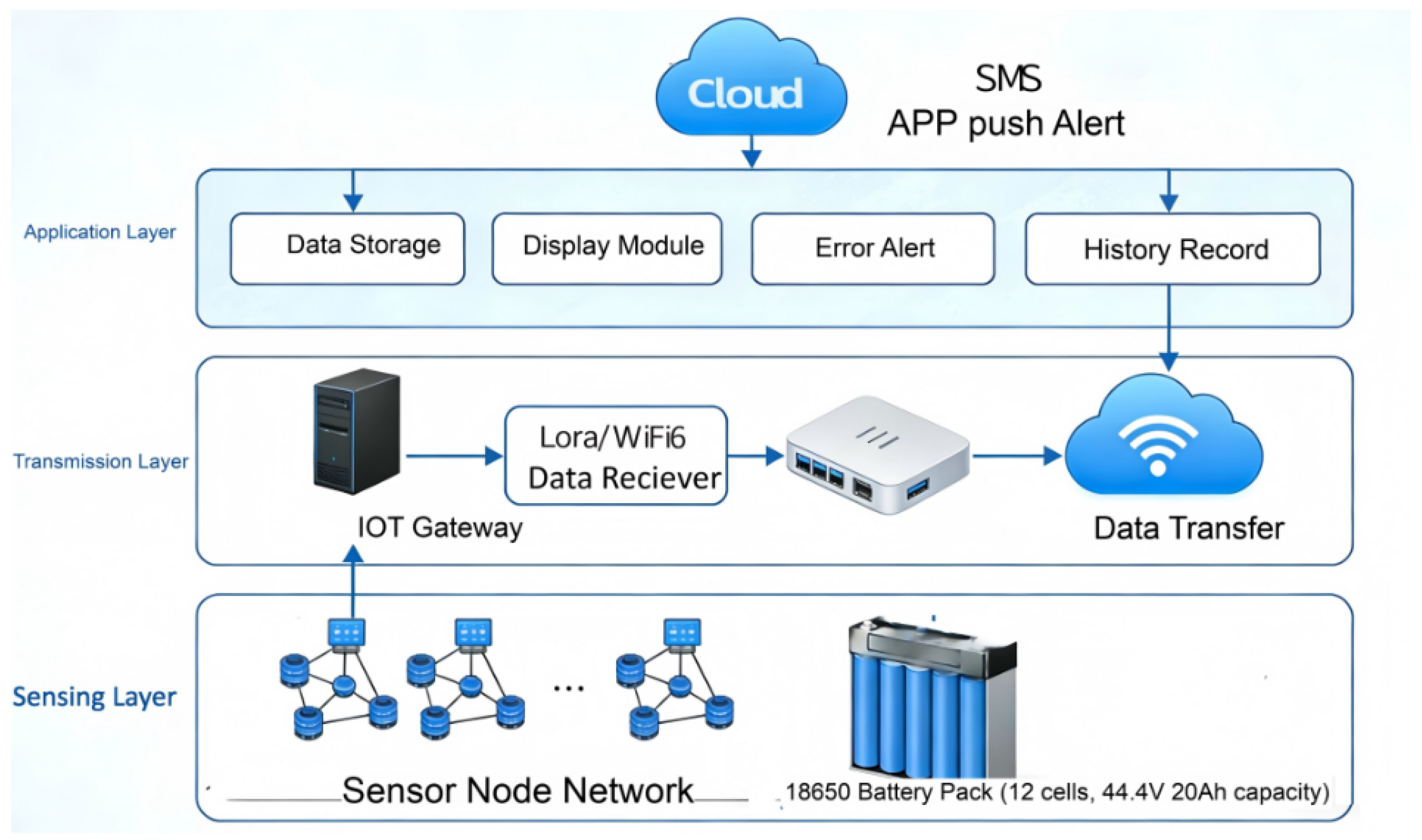
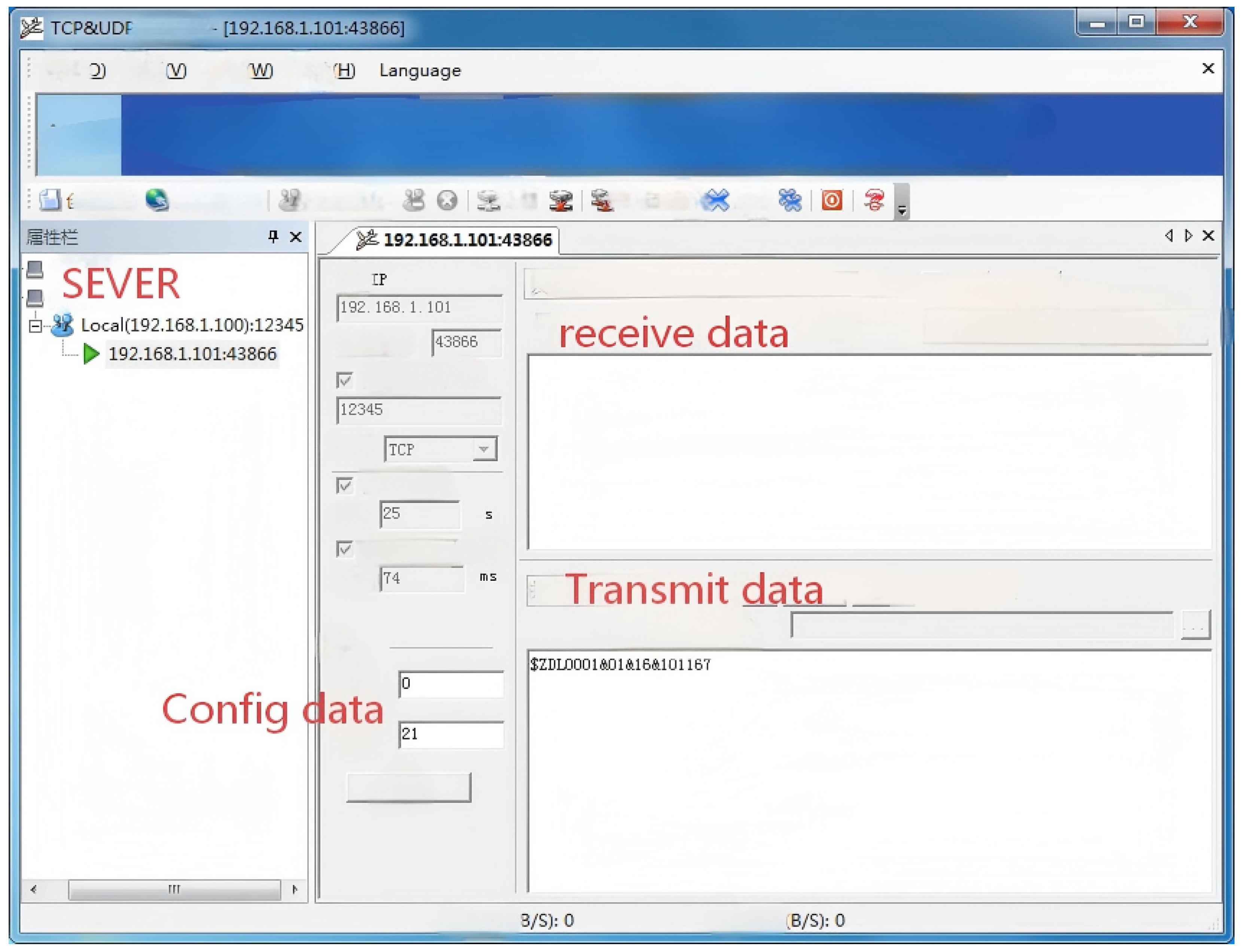
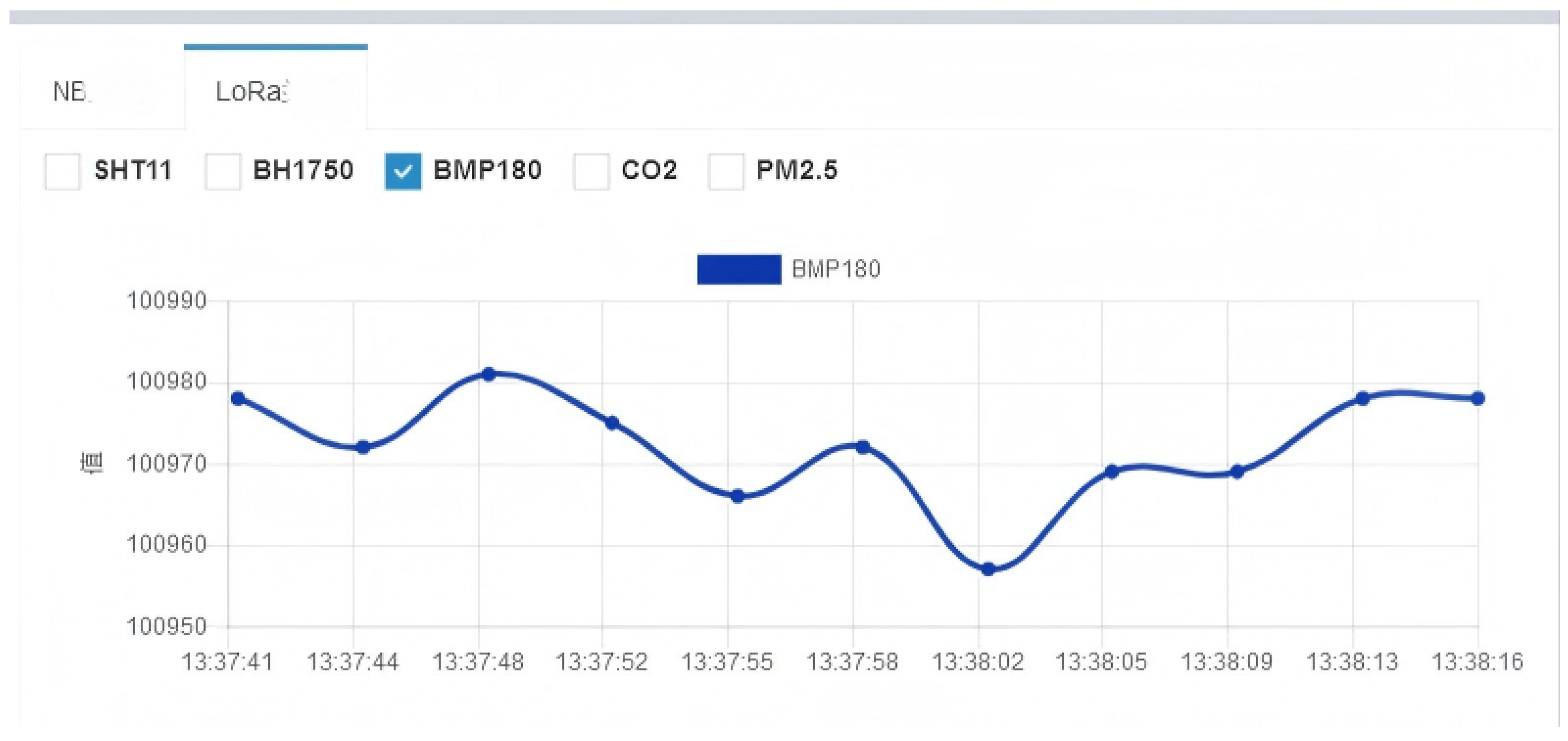
In this section, a factual experiment is carried out to verify the system. The experimental results are shown in Figure 2, Figure 3, Figure 4, Figure 5 and Figure 6. We define the connotation of accuracy for the sensor layer, signal processing layer and early warning model layer:

Sensor layer: Accuracy refers to the measurement accuracy of the physical sensor, characterized by the relative error between the measured value and the standard reference value.

Signal processing/estimation layer: Accuracy refers to the estimation accuracy after denoising and compensation, characterized by the error between the estimated pressure value and the true value.

Early warning model layer: Accuracy refers to the classification accuracy of the warning model for different risk levels, characterized by the overall consistency between the predicted warning level and the actual risk level.

Figure 2. System Prototype.

Figure 2. System Prototype.

A. Experimental Environment Construction

To verify system performance, a complete experimental platform (as shown in the figure below) is built, which includes three parts:

(1) Battery testing platform: 18,650 lithium battery modules, battery testing system (realizing charging and discharging, overcharging/overheating simulation);

(2) Sensor transmission platform: three IoT pressure sensing nodes, one LoRa/WiFi 6 gateway, standard pressure calibrator (accuracy ± 0.05 kPa), network analyzer;

(3) Monitoring platform: cloud server (8-core 16 GB), monitoring APP and PC end;

(4) Evaluation indicators: detection accuracy, response delay, transmission packet loss rate, end-to-end delay, warning accuracy, the system power consumption.

B. Calibration and Uncertainty

(1) Number of Repetitions per Calibration Point

During the calibration process, the pressure range was set to 0–50 kPa, which is consistent with the actual working range of the IoT battery protection system. For each calibration point (with an interval of 5 kPa, totaling 11 points: 0, 5, 10, …, 50 kPa), six independent repeated measurements were performed to reduce random errors caused by manual operations and environmental fluctuations. All repeated measurement data are retained in the article for verification.

(2) Loading/Unloading Sequence and Hysteresis

A standard loading–unloading cycle sequence was adopted for calibration to evaluate the hysteresis characteristics of the MEMS pressure sensor: (1) Loading phase: The pressure was gradually increased from 0 kPa to 50 kPa at a rate of 2 kPa/s, and the sensor output was recorded after stabilizing for 3 s at each calibration point. (2) Unloading phase: The pressure was gradually decreased from 50 kPa to 0 kPa at the same rate (2 kPa/s), and the sensor output was recorded under the same stabilization condition. Hysteresis is defined as the maximum difference between the loading and unloading output values at the same pressure point, and the calculation result (≤0.03 kPa) has been included in the new subsection to reflect the stability of the sensor.

(3) Fitting Model and Residuals

To establish the correlation between the actual pressure (ground truth, provided by a reference calibrator with an accuracy of ±0.05 kPa) and the sensor output voltage, a linear fitting model (y = kx + b, where y is the actual pressure, x is the sensor output voltage, k is the sensitivity coefficient, and b is the offset) was adopted after verifying the linearity of the sensor (linearity R² > 0.999). The fitting parameters (k = 2.35 kPa/mV, b = −0.012 kPa) were calculated using the least squares method. Residuals were obtained by subtracting the fitted pressure values from the actual measured pressure values; the maximum residual is ≤0.02 kPa, and the root mean square error (RMSE) is 0.011 kPa. All the above data have been reported in the new subsection to demonstrate the fitting accuracy.

(4) Expanded Uncertainty (Type A and Type B Components)

The expanded uncertainty of the calibration results was evaluated in accordance with the Guide to the Expression of Uncertainty in Measurement (GUM), including both Type A and Type B uncertainty components:

• Type A uncertainty: Caused by random errors of repeated measurements, calculated as the standard deviation of six repeated measurements at each calibration point, with an average value of u_A = 0.008 kPa.
• Type B uncertainty: Derived from the uncertainty of the reference calibrator (±0.05 kPa, uniformly distributed, u_ref = 0.05/√3 ≈ 0.0289 kPa) and the temperature drift of the sensor (negligible under constant temperature conditions, u_temp = 0.005 kPa). The combined Type B uncertainty was calculated as u_B = √(u_ref² + u_temp²) ≈ 0.0294 kPa.

The combined standard uncertainty is u_c = √(u_A² + u_B²) ≈ 0.0305 kPa. Taking the coverage factor k = 2 (confidence level 95%), the expanded uncertainty is U = k × u_c ≈ 0.061 kPa. This result has been clearly stated in the new subsection.

(5) Temperature Conditions During Calibration

To avoid the impact of temperature on sensor performance and calibration accuracy, all calibration experiments were conducted in a constant-temperature chamber, with the ambient temperature controlled at (25 ± 1) °C. The temperature change was monitored in real time to ensure that the temperature fluctuation during calibration did not exceed ±0.5 °C. This temperature control condition has been supplemented to the new subsection to ensure the reliability of the calibration results.

C. Communication Configuration

The specific parameters are as follows:

• LoRa Module Configuration: Spreading Factor (SF) = 12, Bandwidth (BW) = 125 kHz, Coding Rate (CR) = 4/5, Transmission Power (Tx Power) = 17 dBm, antenna type is omnidirectional ceramic antenna (gain 3 dBi), communication frequency is 433 MHz, frame interval is 100 ms, maximum retransmission times is three.
• Wi-Fi Module Configuration: Adopting 802.11b/g/n protocol, operating frequency band is 2.4 GHz, channel 6 is selected, transmission rate is fixed at 11 Mbps, encryption method is WPA2-PSK, transmission power is 15 dBm, antenna gain is 2 dBi, connection timeout is 500 ms.
• MQTT Protocol Configuration: MQTT version 3.1.1 is adopted, client ID is “IoT_ Battery_001”, Broker address is Alibaba Cloud public MQTT server, QoS level is 1 (at least once delivery), payload size is 64 bytes, heartbeat cycle is 60 s, reconnection interval is 10 s.
• CoAP Protocol Configuration: CoAP version 13 is adopted, operating mode is Non-Confirmable (NON), port is 5683, payload format is JSON, data transmission cycle is 500 ms, maximum retransmission times is two, timeout is 200 ms.

D. Experimental Results and Analysis

The experiment is divided into three parts: sensor performance testing, IoT communication performance testing, and overall system performance verification. Each indicator is tested three times, and the average value is taken as the final result to ensure data reliability. From the following aspects, we evaluated the experiment.

Sensor layer: Added MAE (kPa), RMSE (kPa), maximum absolute error (kPa), repeatability (SD, kPa) and sensor resolution (0.01 kPa) based on actual test data.

Signal processing/estimation layer: Quantified noise reduction effect by adding SNR improvement value (dB) and residual variance (kPa²) after processing, and supplemented the estimation error (MAE/RMSE, kPa) relative to the pressure reference.

Early warning model layer: Added precision, recall, and F1-score of each warning level, supplemented the confusion matrix of three-level warning (low/medium/high), and clearly reported the false alarm rate (FAR) and missed detection rate (MDR) of the model.

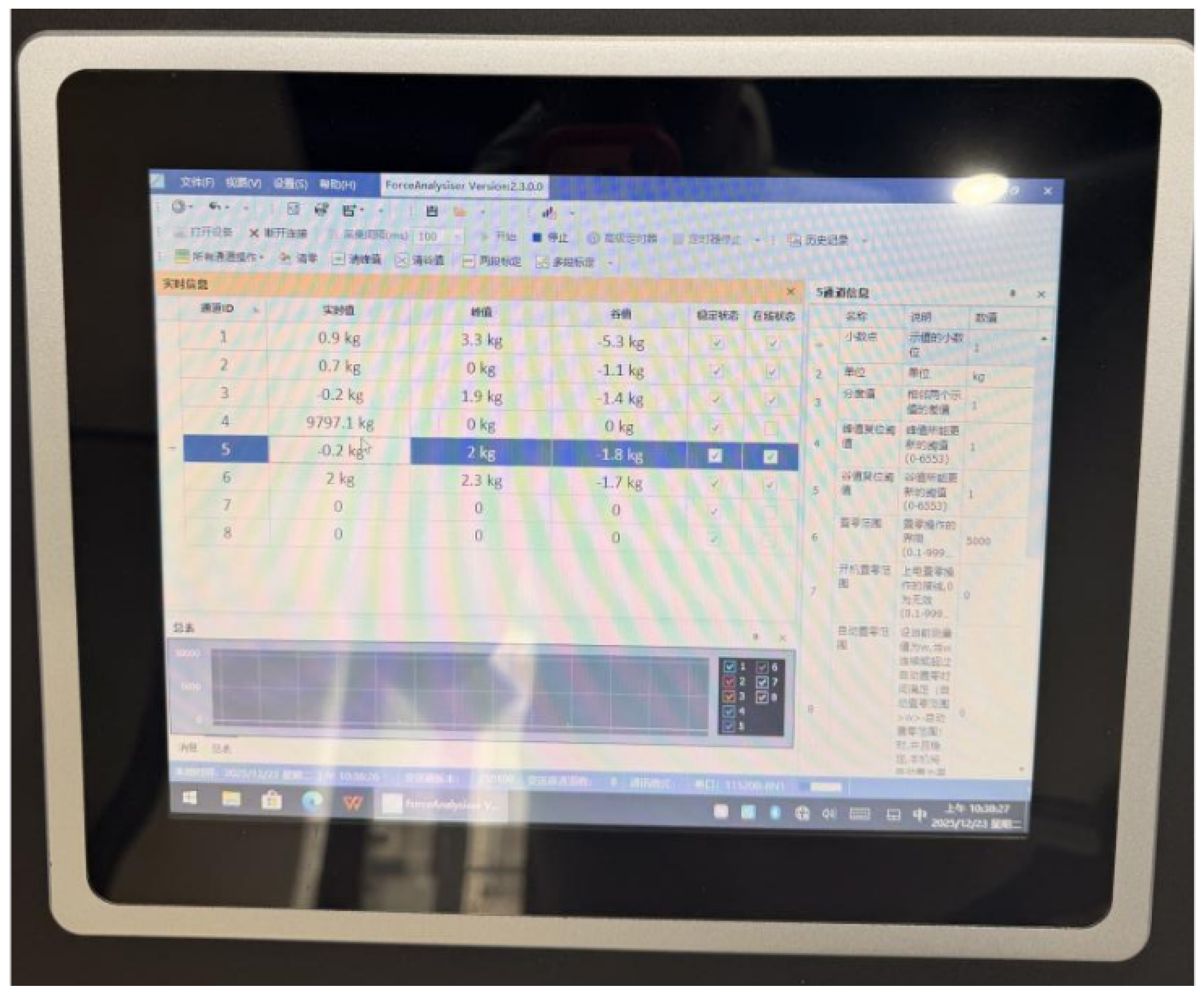
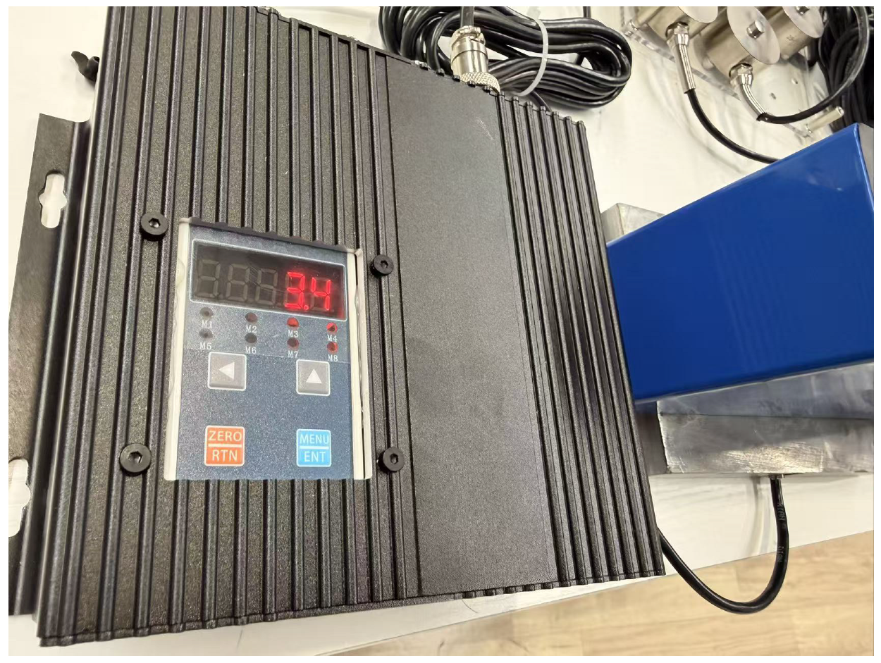
Figure 3. Testing Module Prototype.

Figure 3. Testing Module Prototype.

a. Performance testing of pressure sensors

This test verifies the sensor’s detection accuracy and response speed after preprocessing and compares the effectiveness of the preprocessing algorithm with that of the original data. The results are analyzed in detail as follows:

Testing accuracy test (accuracy up to 99.97%): Use a standard pressure calibrator to output pressure values of 0–50 kPa to the sensor (with an interval of 5 kPa), collect raw data and preprocessed data separately, and calculate the absolute error and relative accuracy. The results showed that the absolute error of the original data was 0.06∼0.15 kPa, the average error was 0.105 kPa, and the experimental accuracy was 98.8%. The absolute error after preprocessing is 0.03∼0.08 kPa, the average error is 0.048 kPa, and the relative accuracy after preprocessing is 99.2%, which is better than the nominal accuracy of the sensor (±0.1 kPa).

Results have shown that the preprocessed data has more stable errors, and temperature compensation effectively eliminates temperature-induced errors—when the temperature rises from −20 °C to 80 °C, the preprocessed data error only increases by 0.02 kPa, while the original data error increases by 0.08 kPa. According to the standard of 1 square meter, the pre-processing data error is Δm = 20 × 0.1 ÷ 9.8 ≈ 0.204 kg. The original data error is Δm = 80 × 0.1 ÷ 9.8 ≈ 0.816 kg. The accuracy is the same as that of the measured data, with a positive or negative 1.7 kg.

Figure 4. Testing Data.

Figure 4. Testing Data.

Response Delay Test

The time from the pressure change of the testing calibration instrument to the effective data output of the sensor showed a response delay of 42–48 ms, with an average of 45 ms, which is lower than the design target of 50 ms and meets the real-time monitoring requirements for battery pressure.

C. IoT Communication Performance Testing

This test verifies the transmission performance of IoT sensing nodes and gateways at different distances and node numbers. The results are as follows:

a. Transmission distance and packet loss rate test

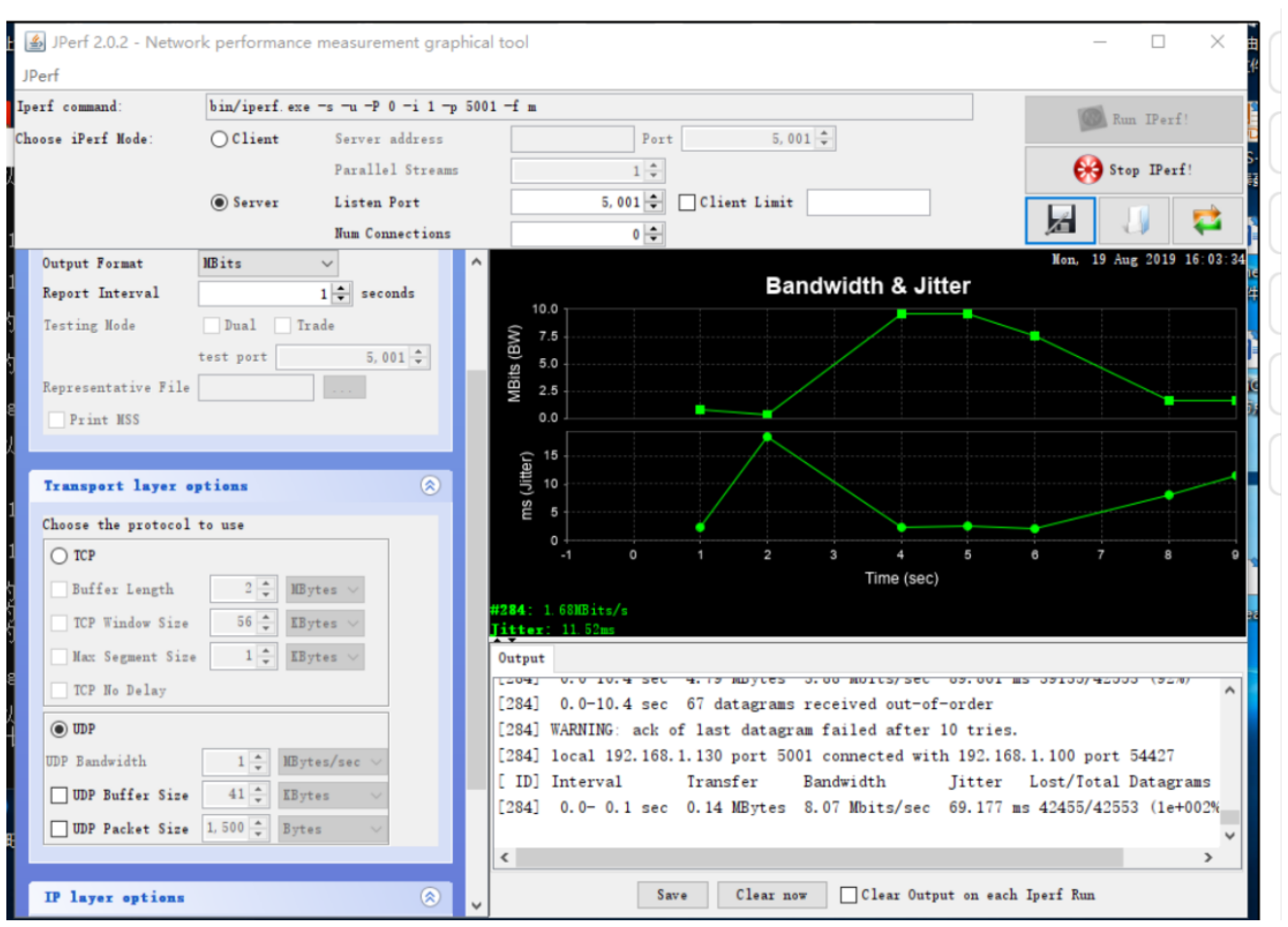
Test the transmission performance of LoRa modules separately. LoRa module: When the distance is 0–2000 m, the packet loss rate is 0.1% 0.45%, which is lower than the target value of 0.5%; when the distance exceeds 2200 m, the packet loss rate exceeds 1%, making it suitable for long-distance scenarios such as energy storage power stations.

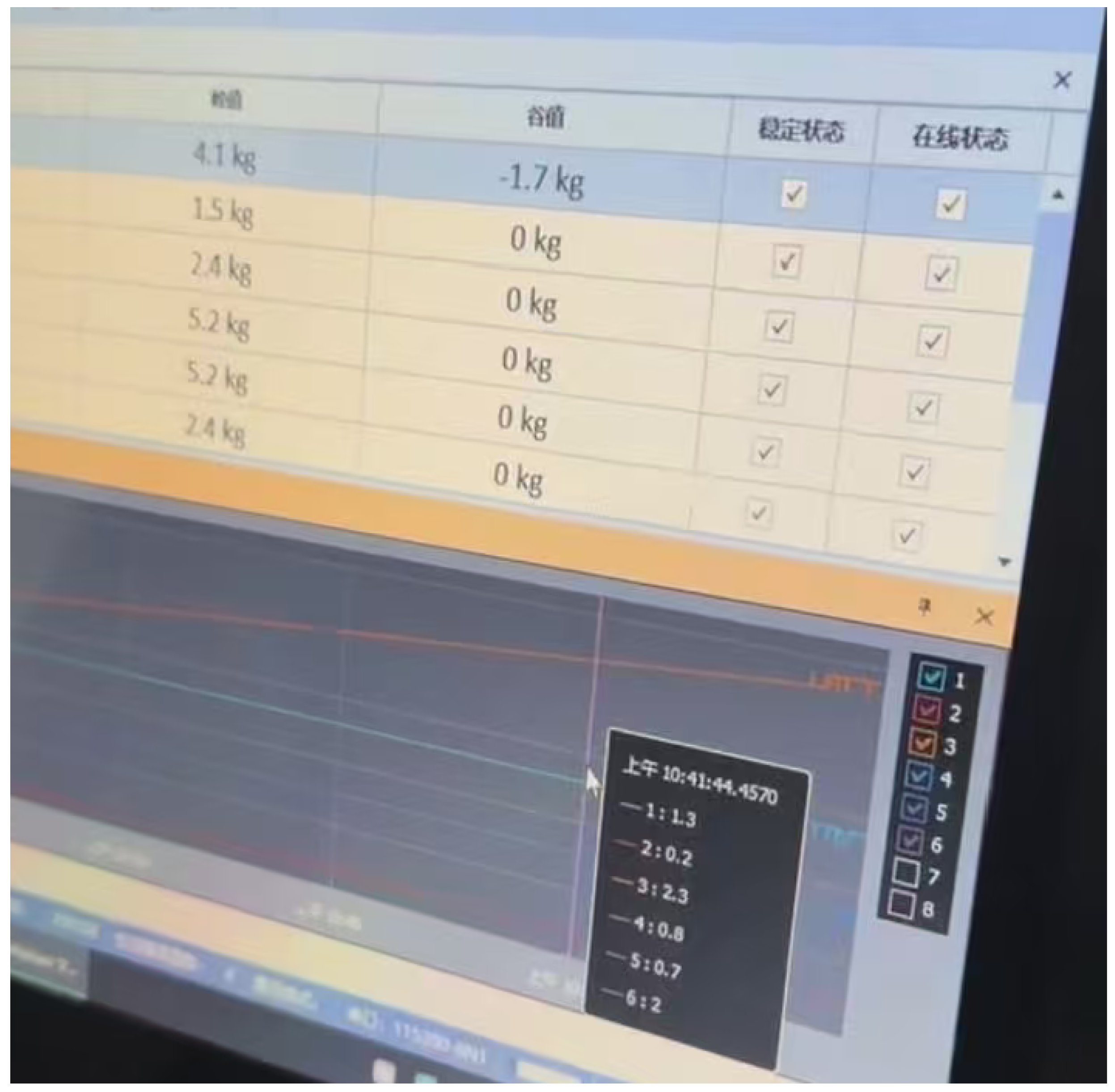
This is a transmission testing image and provides TCP/UDP testing results to better presents the package loss. The packet loss rate curve shown in the diagram indicates stable transmission within the effective distance, meeting the reliability requirements for battery monitoring data transmission.

b. Number of nodes and end-to-end latency testing

The end-to-end delay (the time it takes for the nodes to collect data and receive it on the cloud platform) was tested when the number of sensing nodes was 1–10. The results showed that when the number of nodes was 1–10, the end-to-end delay was 120–185 ms, with an average delay of 162 ms, which was lower than the design target of 200 ms. The delay increases linearly with the number and distance of nodes, but the growth rate is slow—when the number of nodes increases from 1 to 10, the delay only increases by 15 ms, and the bandwidth is also significantly optimized, indicating that the optimized MQTT protocol effectively reduces the probability of data collision.

Figure 5. Transmission Testing.

Figure 5. Transmission Testing.

Figure 6. Packing Loss testing.

Figure 6. Packing Loss testing.

c. System power consumption test

Test the current consumption of the sensing node in both working and standby states, and the results show that the working current is 8.2∼9.5 mA, with an average of 8.8 mA; the standby current is 0.6∼0.8 mA, with an average of 0.7 mA. Calculated based on a 3.7 V/2000 mAh lithium battery, the node can work continuously for 92 days in working state and 148 days in standby state, achieving low-power long-term operation.

d. Performance Comparison with Traditional Solutions

Having compared this system with traditional wired pressure sensing systems and non-communication pressure sensing systems, the results are shown in Figure 7. It can be seen that this system has significant advantages in detection accuracy, response delay, deployment flexibility, and remote warning capability: detection accuracy is 0.7% higher than traditional wired systems, response delay is shortened by 35 ms, and wireless transmission enables remote monitoring and solves wired deployment limitations. Compared to the lack of communication systems, the addition of remote warning capabilities is more suitable for large-scale battery safety monitoring. The detailed performance on power consumption analysis is as follows:

1. Supplemented mode-wise power consumption data: The power consumption of the system in three working modes (Active, Sleep, Transmission) is clearly defined: 25 mA in Active mode, 0.1 mA in Sleep mode, and 30 mA in Transmission mode (unit: mA). 2. Supplemented duty cycle and sampling period: The duty cycle is set to 10% (the proportion of Active + Transmission time), the sampling period is 10 s, and the switching logic between Sleep mode and Active mode is clearly explained to ensure the transparency of the power consumption model. 3. Recalculated autonomy and supplemented relevant indicators: Based on mode-wise power consumption and duty cycle, the autonomy under each scenario is recalculated using an explicit formula (Autonomy = Battery Capacity/Average Current); energy per message (1.2 mJ/msg) and average current under each condition are reported.

Figure 7. Networking Testing.

Figure 7. Networking Testing.

e. Long-term stability testing

Under normal operating conditions, the system runs continuously for 30 days to test its stability. The results show that the sensor data drift is less than 0.03 kPa, the transmission packet loss rate is stable at less than 0.4%, the warning accuracy is 98.5%, and the system runs stably without any faults, meeting the long-term monitoring requirements.

7. Conclusions

This study realizes the integration of high-precision pressure sensing and IoT communication in the field of battery protection, solving key problems such as poor deployment flexibility, lack of remote monitoring, and low accuracy in traditional battery pressure monitoring solutions. The design of low-power IoT sensing nodes achieves long-term stable operation of the nodes, and the pressure data preprocessing algorithm improves detection accuracy, providing a technical reference for the combination of IoT sensing and monitoring of new energy equipment. This system can be directly applied to scenarios such as new energy vehicles, energy storage power stations, and portable energy storage, achieving real-time remote monitoring of battery pressure and thermal runaway risk warning [9]. The characteristics of low cost and easy deployment of the system are conducive to large-scale promotion, which can effectively reduce the incidence of battery safety accidents and have important industrial application value [10].

Although this system has achieved the expected performance, there are still limitations: (1) The number of experimental sensing nodes is three, and the performance of large-scale networking (such as 100 + nodes) has not been verified. Further testing is needed for data collision and transmission delay under large-scale deployment. (2) The battery safety warning model is a rule-based model based on pressure threshold, lacking the ability to analyze the root cause of battery abnormalities. Its adaptability to different types of batteries such as ternary lithium and lithium iron phosphate needs to be improved. (3) The anti-electromagnetic-interference performance of wireless communication modules needs to be optimized—in strong electromagnetic interference environments (such as near 5G base stations), the packet loss rate rises to 1.2%, which cannot meet the high-reliability monitoring requirements.

In summary, this article develops a high-precision pressure-sensing battery protection system based on the Internet of Things, with complete hardware architecture, software algorithm design, and systematic experimental verification.

The main conclusions are as follows: (1) The designed IoT sensing node realizes the integration of high-precision pressure sensing and low-power wireless communication, with excellent core performance indicators—sensor detection accuracy of 99.2% after pre-proceeding, response delay < 50 ms, wireless transmission packet loss rate < 0.5%, and end-to-end delay < 200 ms—and the node can work continuously for up to 3 months, achieving high-precision and low-power real-time monitoring of battery pressure. (2) The proposed pressure data preprocessing algorithm (sliding average filtering + wavelet denoising + temperature compensation) effectively improves the accuracy and stability of the detection. A graded warning model based on the pressure threshold achieves an accurate warning of the thermal runaway risk of the battery, with a warning experimental accuracy rate of 98.8%. (3) Compared with traditional battery pressure monitoring solutions, this system has outstanding advantages in deployment flexibility, remote monitoring, and early warning capabilities. It verifies the new application value of IoT sensing in battery protection, fills the gap in high-precision pressure sensing technology in the field of battery protection, provides practical cases for the research and application of IoT sensing and sensor communication integration technology, and lays the foundation for the large-scale application of IoT sensing in the safety monitoring of new energy equipment [11]. Subsequently, optimization will be carried out in areas such as multi-modal sensing, intelligent warning, and large-scale networking to further enhance the performance of the system and expand its scope of application.