Article

A Hybrid-Driven Fault Diagnosis Method for Railway Freight Car Braking System

1
School of Computer Science and Technology, Beijing Jiaotong University, Beijing 100044, China
2
Engineering Research Center of Network Management Technology for High Speed Railway, Ministry of Education, Beijing 100044, China
*
Author to whom correspondence should be addressed.
Electronics 2026, 15(4), 895; https://doi.org/10.3390/electronics15040895
Submission received: 31 December 2025 / Revised: 6 February 2026 / Accepted: 10 February 2026 / Published: 21 February 2026

Abstract

With the increasing demand for heavy-haul railway freight, both the number and volume of heavy-haul freight cars continue to grow. As the core system of railway freight transportation, the reliable operation of the brake system is fundamental to ensuring train safety. The freight car braking system fault diagnosis model, which relies on historical data while failing to account for changes in braking curves when locomotives are coupled with different vehicles, is the main reason why early failures of the braking system are not diagnosed. Consequently, real-time monitoring of the freight car braking system and early fault diagnosis have emerged as a pivotal technical challenge that necessitates resolution within the framework of the railway freight maintenance reform. This paper proposes a novel hybrid-driven prediction method that effectively combines Convolutional Neural Networks, Adaptive Radial Basis Function Neural Networks, and Extreme Learning Machines (CARE). To achieve comprehensive fault feature extraction, based on CNN of the image data classification, the K-means clustering algorithm is introduced to adaptively initialize the radial basis centers of the RBF and recalculate the radial basis radii. Moreover, to improve the real-time performance and accuracy of fault diagnosis, the network layers are expanded, and the ELM algorithm is employed to construct an optimization strategy for high-dimensional data processing in the network layers. The experimental results demonstrate that when considering the coupling of different vehicles in the railway freight car, the proposed CARE model exhibits faster convergence speed and significantly improves the effectiveness and real-time performance of fault diagnosis in the railway freight car braking system.

1. Introduction

As a large-scale transportation vehicle, the demand for railway freight car transport continues to grow. With the enhancement of transport capacity, the reliability and safety of train systems are facing increasingly higher requirements. However, due to potential technical anomalies and failures of critical components, train systems still frequently experience faults, which in turn affect transportation efficiency [1].
To prevent significant losses caused by equipment failures, the maintenance of train systems has gradually shifted from post-failure repairs (conducted after a fault occurs) and periodic maintenance to Condition Based Maintenance (CBM). By leveraging data from trackside and onboard sensors, CBM enables real-time analysis of vehicle status and operational conditions, allowing for early detection and identification of any potential anomalies or faults. This approach facilitates dynamic planning of maintenance schedules and repair activities, avoiding both “under-maintenance” and “over-maintenance.” As a result, it reduces maintenance costs, ensures operational safety, extends the service life of vehicle components, and enhances the economic efficiency of enterprises [2].
Railway freight cars are composed of seven major subsystems that work in coordination: the car body, underframe, bogie, foundation brake equipment, air brake equipment, coupler and buffer system, and wheel-axle assembly. Among these, the foundation brake equipment and air brake equipment combine to form the railway freight car brake system. A stable and reliable braking system is indispensable for driving safety, as it can smoothly and promptly decelerate or bring the vehicle to a halt when needed. Over the past few decades, Prognostics and Health Management (PHM) technology has been applied in fields such as aviation and railways, aiming to enhance system reliability and reduce maintenance costs [3]. As one of the most common activities in PHM, fault diagnosis of railway freight car braking systems evaluates the current health status of the braking system to prevent sudden failures. It assists on-site personnel in reasonably arranging maintenance resources, timing, and reducing maintenance costs [4,5]. Currently, fault diagnosis of braking systems can be categorized into three types: model-based analytical methods, knowledge-based methods, and data-driven methods [6]. Specifically, the model-based analytical methods rely on the principles of the braking system and sensor data to establish physical models, such as air fluid theory and linear matrix inequalities, but they cannot be generalized to actual complex working conditions [7,8]. The knowledge-based methods depend on expert knowledge to construct nonlinear classification models for the braking system, such as fault trees and Bayesian network models [9,10]. However, due to the influence of expert knowledge and model builders, these methods currently remain at the theoretical stage.
With the rapid expansion of sensor data collected from railway tracks and locomotives, data-driven methods have become popular in fault diagnosis. These methods establish mathematical models by deeply mining the features of historical and real-time data from multiple sensors. This approach not only avoids the poor performance of mathematical or physical models in complex working conditions but also mitigates the issue of significant errors in models constructed based on expert experience [11]. Due to the remarkable capability of CNNs in extracting image features, many researchers have widely integrated CNNs with other artificial neural networks for fault diagnosis. For instance, Chen et al. [12] investigated the integration of CNNs with Long Short-Term Memory (LSTM) networks to develop a bearing fault diagnosis system based on depth information and historical data. Zhang Yahui et al. [13] addressed the issue of temporal information loss in CNNs for fault diagnosis by incorporating Gated Recurrent Units (GRU). Although LSTM and GRU architectures excel in processing long-range dependencies, their intricate gate mechanisms entail a substantial parameter burden and prolonged training times. Furthermore, they remain susceptible to gradient vanishing when processing high-dimensional inputs, such as braking curve images. Consequently, these limitations pose a bottleneck for fault diagnosis in the braking systems of railway freight cars, where immediate response is critical. In contrast, Radial Basis Function (RBF) neural networks, characterized by their simple forward structure and robust local approximation capabilities, are widely utilized in mechanical diagnostics for their efficiency in performing non-linear mapping and fault classification based on real-time equipment states. Wang Pengbo et al. [14] employed RBF for the mechanical fault diagnosis of gearboxes. Wang Jia et al. [15] utilized an improved RBF network for detecting faults in lithium batteries. However, traditional RBF networks often struggle with the high-dimensional feature extraction required for complex image data. Therefore, this study proposes a novel hybrid framework that synergizes the high-dimensional abstract feature extraction capability of CNNs with the rapid classification speed of RBF networks. Unlike LSTM-CNN hybrid models that may incur significant computational overhead, our optimized approach is designed to extract high-dimensional abstract features from braking curve images while facilitating real-time fault diagnosis.
This study focuses on the historical and real-time data collected from the Control Unit (CCU) and Monitoring Unit (ATP) of heavy-haul railway train braking systems. By analyzing the pressure variation mechanisms during fault processes in braking systems under different scenarios of multiple locomotives with varying numbers of connected freight cars, the research proposes an adaptive train fault diagnosis optimization model, CARE, specifically designed for real-time fault diagnosis in braking systems. Addressing the critical challenges of low fault classification performance and significant diagnostic delays in practical engineering applications, this model significantly enhances the accuracy and robustness of fault diagnosis. Consequently, it ensures the safe and efficient operation of freight cars while boosting transportation efficiency. This work represents a meaningful contribution to the advancement of preventive CBM. Experimental validation confirms that the CARE fault diagnosis model demonstrates superior performance and classification effectiveness.
The remainder of this paper is organized as follows. The Section 2 on foundational theory and technical research introduces the theoretical foundations and related technologies underlying the proposed method. The next Section 3 presents a detailed description of the fault diagnosis model and the application of CARE. The experimental Section 4 describes the dataset and reports the results of comparative experiments. Finally, the conclusion Section 5 summarizes the findings and outlines directions for future work.

2. Foundational Theory and Technical Research

2.1. Principles of Braking Systems and Fault Classification

With the continuous advancement of rail transit technology, the braking systems in railways have become increasingly complex. However, the railway freight cars continue to utilize braking systems characterized by simplicity and reliability. The braking system of freight cars consists of several key components, including the main reservoir, train line, auxiliary reservoir, brake cylinder, and brake shoe. The main reservoir is situated within the locomotive and is connected to the train line. This train line is subsequently linked to the braking system of each following vehicle, thereby constituting the overall braking system of the train. Figure 1 provides a detailed depiction of the braking mechanism employed in the railway freight car braking system.
The braking system of freight cars is interconnected through a pressurized pipeline, known as the train line, which links the locomotive with all the vehicles, employing a pressure reduction braking mechanism. As the pressure in the train line decreases relative to the brake cylinder, the triple valve shifts to the right until the pressure in the auxiliary reservoir approximates that of the train line. Concurrently, the auxiliary reservoir connects to the brake cylinder, which then disconnects from the atmosphere. At this juncture, the air pressure within the brake cylinder propels the piston forward, forcing the brake shoe against the wheel tread to achieve braking [16].
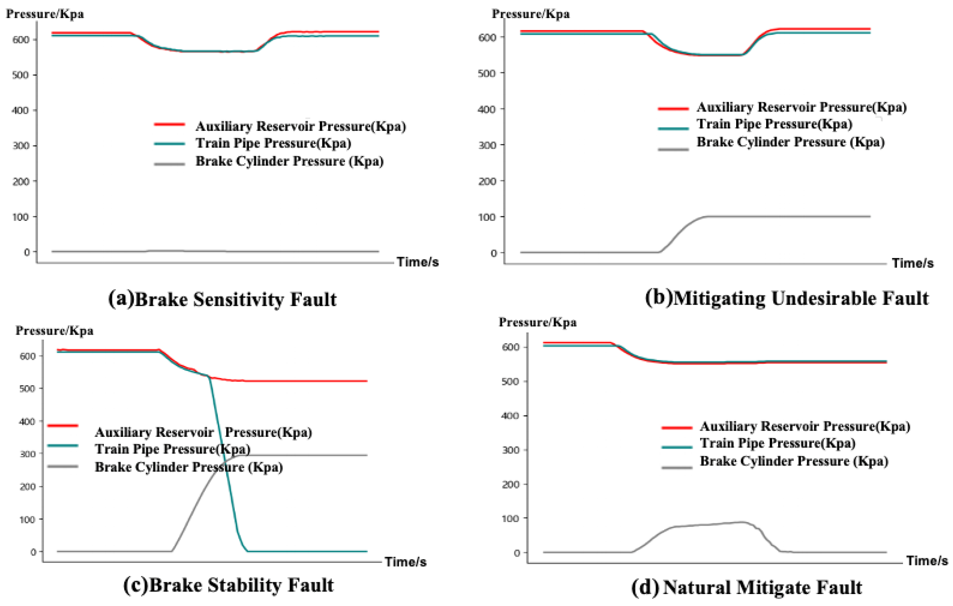
Due to the fault of critical braking components such as the triple valve and brake cylinder, abnormal pressure variations occur in the auxiliary reservoir, train line, and brake cylinder during train braking. Consequently, train braking faults can be categorized into four types: brake sensitivity fault, mitigating undesirable fault, brake stability fault, and natural mitigate fault. The braking curves for these four types of failures are illustrated in Figure 2.
1.
Brake Sensitivity Fault: When a minimum braking pressure reduction of 40 kPa is applied, the brake cylinder pressure does not exhibit a significant change. This may be attributed to faults in the brake cylinder or triple valve, resulting in the inability to generate effective braking force, as illustrated in Figure 2a.
2.
Mitigating Undesirable Fault: When the train handle is set to the release position, the train line pressure and auxiliary reservoir pressure increase due to the charging pressure from the main reservoir. However, the train line pressure does not decrease as expected. This issue may arise from a fault in the triple valve, preventing the brake cylinder from venting to the atmosphere, as illustrated in Figure 2b.
3.
Brake Stability Fault: When the maximum pressure reduction is applied during train braking, the train line pressure abnormally drops to 0 kPa, triggering an emergency brake. This situation may occur due to loose connections in the train line or inherent faults in the train line itself, causing the brake cylinder to be charged to its maximum pressure by the auxiliary reservoir. At this point, the auxiliary reservoir pressure stabilizes after reaching the maximum reduction level, as illustrated in Figure 2c.
4.
Natural Mitigate Fault: When the train brake handle remains in the braking position, the brake cylinder pressure decreases unexpectedly. This may be caused by a fault in the brake cylinder, with the triple valve in the holding position, resulting in a relative equilibrium between the train line and auxiliary reservoir pressures, as illustrated in Figure 2d.

2.2. Convolutional Neural Network (CNN)

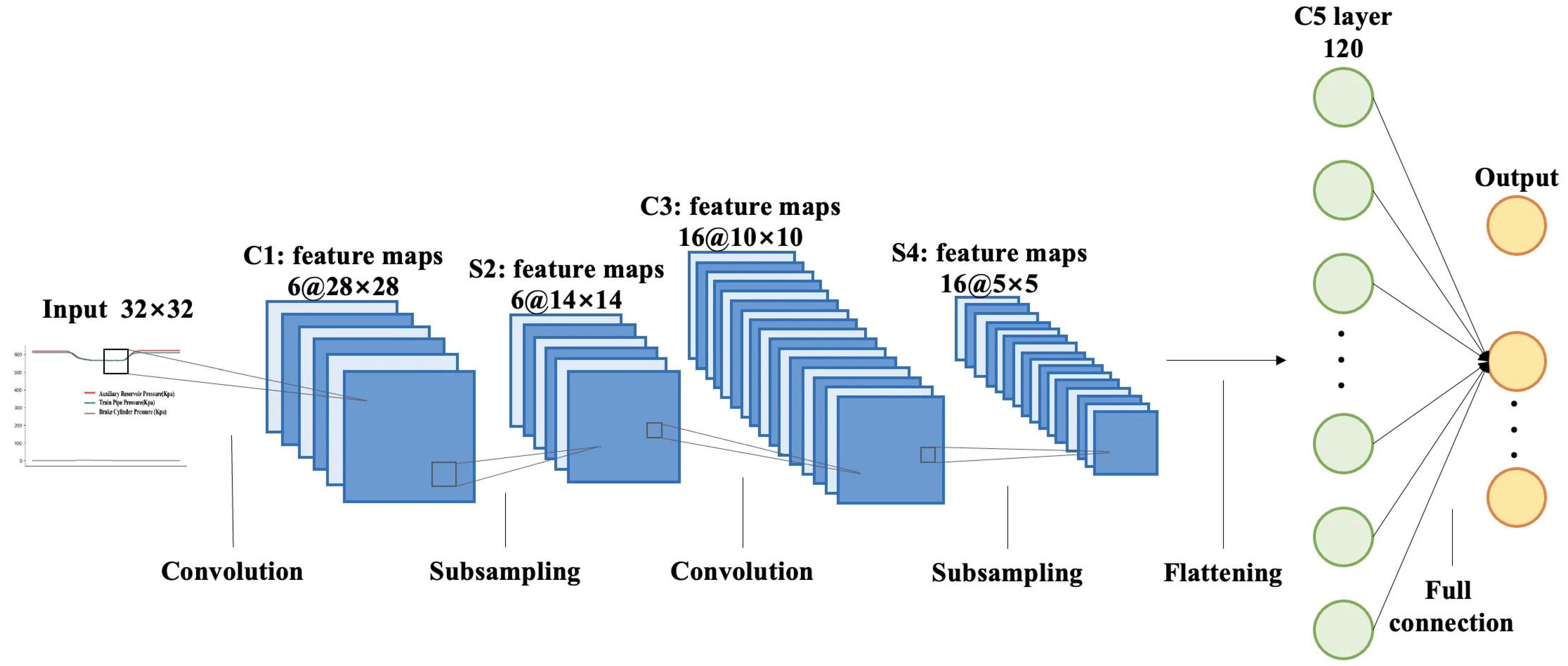
The braking fault curves of the train exhibit significant variations in their patterns depending on the type of fault. Therefore, this study utilizes a Convolutional Neural Network (CNN), which demonstrates strong capabilities in feature extraction from images, to reduce the dimensionality of high-resolution image data. The basic architecture of the CNN, as depicted in Figure 3, typically includes convolutional layers, pooling layers, and fully connected layers at the end of the network to further reduce the dimensionality of the extracted features.

2.3. Radial Basis Function Neural Network (RBF)

RBF is widely applied in various domains, including function approximation, pattern recognition, time series prediction, regression analysis, dimensionality reduction, and anomaly detection, demonstrating excellent capabilities in handling data classification tasks [17]. Additionally, it features a single hidden layer structure. The hidden layer employs different kernel functions as activation functions, enabling rapid network training. The output layer expression y p of the RBF is presented in Equation (1), as follows:
y p = n = 1 N w j k Φ j
where N represents the number of neurons in the hidden layer, w j k denotes the weight value connecting the j-th neuron to the k-th output layer, and Φ j signifies the output value of the j-th neuron in the hidden layer. Since different kernel functions are employed as activation functions in the hidden layer, the choice of kernel function for neuron output significantly influences the model’s fitting performance. The primary kernel functions utilized in RBF networks include the Gaussian Kernel [18], Multiquadric Kernel [19], Linear Kernel [20], and Polynomial Kernel [21]. Among these, the Gaussian Kernel, due to its favorable mathematical properties and versatility, excels in addressing function approximation problems. By controlling the width of the basis functions, it enhances the generalization capability of the RBF network, making it the most frequently used kernel function in RBF applications.

3. Fault Diagnosis Model and Application of CARE

3.1. The Adaptive CNN-ARBF Neural Network (CAR)

The image data of the train braking system is processed through a CNN for feature extraction and subsequently fed into the RBF. To prevent the CNN from excessively reducing the feature dimensionality of the braking curve data, which could lead to the loss of critical feature information, and to address the issue where the selection of Gaussian kernel function centers, the number of centers, and the function width in the RBF hidden layer activation function may cause the RBF to converge to local optima, thereby impairing the data classification performance, the expression of the Gaussian kernel function is provided in Equation (2) as follows:
Φ j ( x ) = exp X C 2 2 σ j 2
In the formula, X represents the input vector, C denotes the center point (or center vector) of the Gaussian function, and σ signifies the width parameter of the Gaussian function.
This paper innovatively proposes an Adaptive Radial Basis Function (ARBF) neural network, which introduces the K-means clustering algorithm to adaptively reconstruct the radial basis centers and radii of the Gaussian kernel function in the RBF hidden layer activation function. This approach efficiently identifies the data centers expanded through the CNN as the centers of the ARBF network. By optimizing the internal structure of the data, the classification performance of the network is enhanced, the risk of overfitting during network training is reduced, and the convergence to local optima is prevented. The adaptive expression for the K-means center clustering is provided in Equation (3) as follows:
A v g ( D j ) = i = 1 N j = 1 K ( x i c j ) 2
where x i represents the feature vector expanded through the CNN, and c j denotes the initialized center. By calculating the mean distance between each point and the center, c j is updated iteratively, ultimately completing the initialization of the Gaussian kernel centers for the RBF network. The adaptive expression for the radial basis width is provided in Equation (4) as follows:
σ j = ( X C ) 2 2 N
where N represents the feature dimensionality of the feature vectors obtained after CNN feature extraction. Based on Equations (3) and (4), the new kernel function expression is derived and presented in Equation (5) as follows:
Φ j ( x ) = exp N ( X C ) 2

3.2. Optimization of the ARBF Algorithm

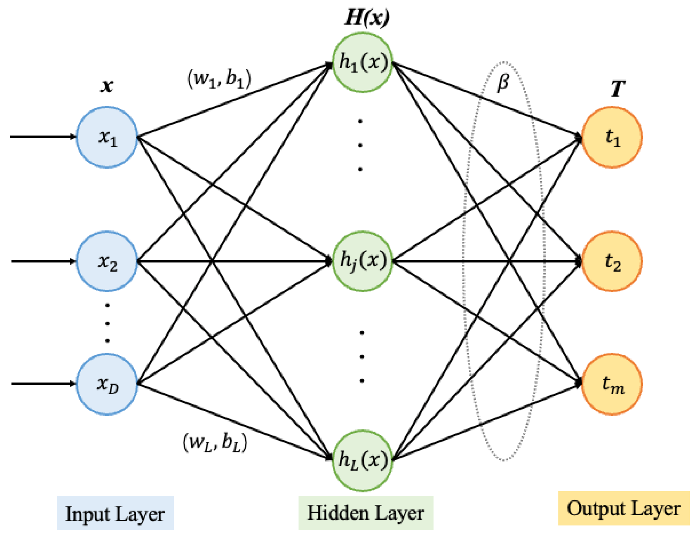
Although the image data of the train braking system retains more feature information after CNN feature extraction, the dimensionality of the feature vectors poses a significant challenge for RBF. To address this, an additional neural network layer is incorporated after the ARBF network, and the ELM algorithm, which exhibits superior generalization capabilities on large-scale datasets compared to deep networks, is employed to optimize the network layer. This enhancement improves the ability of the radial basis function neural network to handle high-dimensional data [22]. The ELM algorithm does not require updating the weights of the input and hidden layers; instead, the output layer weights are computed using the generalized inverse matrix, thereby significantly optimizing the model training speed. Assuming the training set is denoted as { x i , t i x i R D , t i R m , i = 1 , 2 , , N } , where x i represents the i-th input data after processing through the ARBF network, t i represents the label of the i-th input data, and L is the number of hidden layer nodes in the ELM, Figure 4 demonstrates the structure of the ELM network:
The output of the hidden layer in the figure can be expressed as H ( x ) = [ h 1 ( x ) , , h L ( x ) ] , where h i ( x ) represents the activation function applied to f i ( x ) , as shown in Equation (6):
h i ( x ) = g ( w i , b i , x ) = g ( w i f i ( x ) + b i ) , w i R D , b i R
Here, f i ( x ) is defined as a linear function, where w i and b i represent the weights and biases of the hidden layer, respectively. After being processed by the hidden layer, the data advances to the output layer. Consequently, the output expression of the single-hidden-layer feedforward neural network under the ELM can be “generalized” as Equation (7):
f L ( x ) = i = 1 L β i h i ( x ) = H ( x ) β
where β = [ β 1 , , β L ] T denotes the output weights connecting the L hidden layer nodes to the m output layer nodes. The optimization process of the ELM is primarily divided into two stages [23]. During the first step, the hidden layer’s parameters are initialized randomly, mapping the input data into a new feature space, referred to as the ELM feature space. During this stage, the values of w and b are obtained through a uniform random distribution, and the value of the hidden layer output H is computed. In the second stage, to achieve optimal values of β for the training dataset, the training error is minimized by solving for β that reduces the squared difference between H β and the target labels T. The objective function for this optimization is expressed as Equation (8):
min ( H β T ) 2 , β R L × m
where H represents the output matrix of the hidden layer, and T denotes the target matrix of the training data. The expression for H is given by Equation (9) as follows:
H = [ h 1 ( x ) , . . . , h L ( x ) ] T = h 1 ( x 1 ) h L ( x L ) h 1 ( x N ) h L ( x N ) , T = t 1 T t N T
Therefore, the optimal solution for the output weights can be derived as expressed in Equation (10):
β = H T
where H denotes the Moore–Penrose pseudoinverse of the matrix H. The pseudoinverse is solved via Singular Value Decomposition (SVD) to obtain the output layer weights β , which are subsequently combined with Softmax for output layer data classification.

3.3. Application of CARE Framework in Fault Diagnosis of Braking Systems

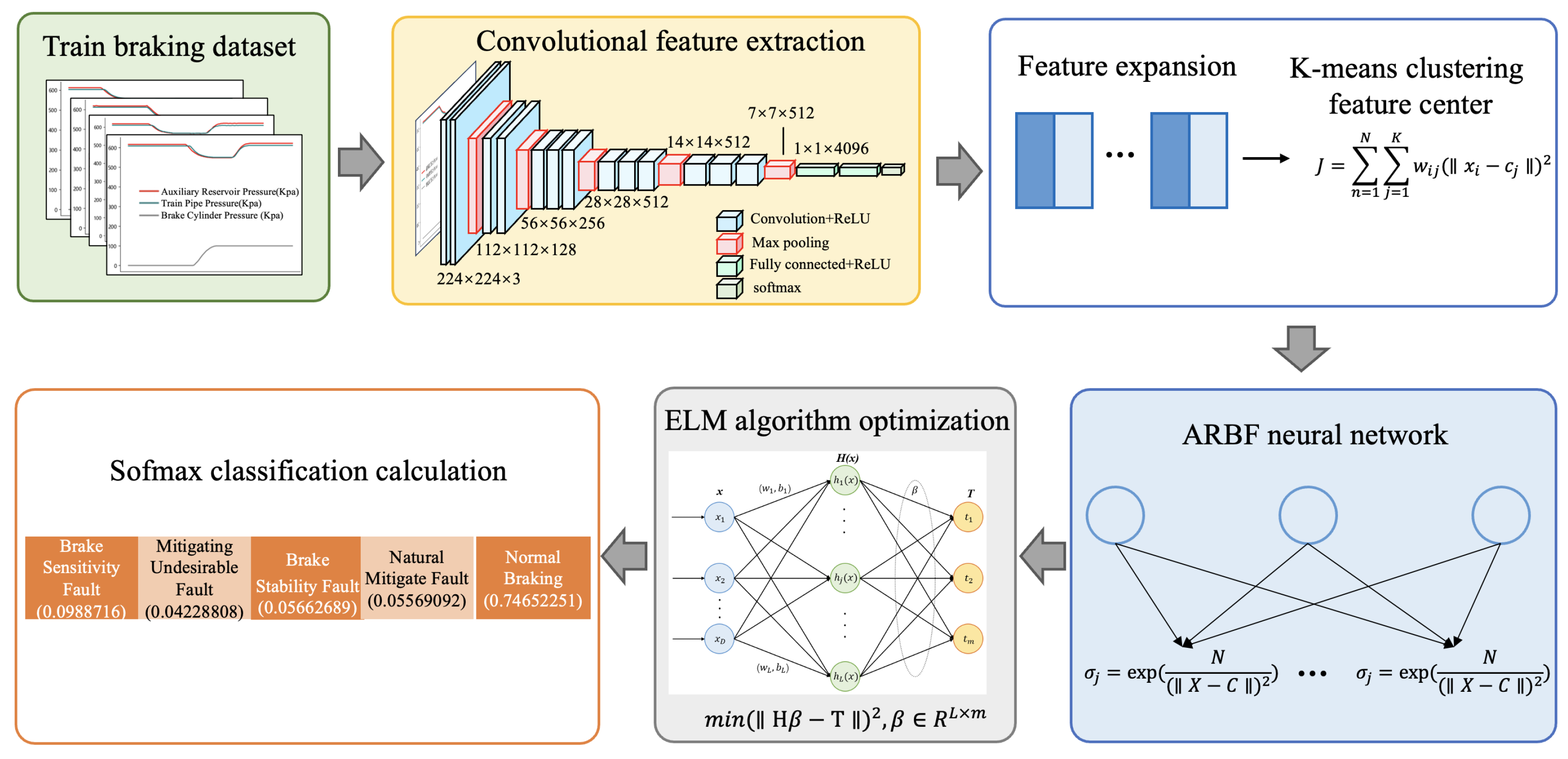
Based on the distinctive features of truck braking process data images, this paper proposes an optimized fault diagnosis framework named CARE, as illustrated in Figure 5.
The image data from the railway freight car braking process is input into the CNN for feature extraction. The K-means algorithm clusters the CNN-derived feature vectors to initialize and determine RBF centers while calculating radial basis function radii. The clustered feature centers, combined with the feature vectors extracted by the CNN, are used to train the ARBF model. The ELM algorithm optimizes the ARBF layer output, with output weights computed via SVD. Finally, a SoftMax classifier is applied to the network’s output to classify and determine the type of braking system fault.

3.4. Evaluation Metrics for the CARE

The fault diagnosis of braking systems investigated in this study belongs to a pattern classification problem. For deep learning classification systems, the classification performance is commonly evaluated using the following metrics:
  • The Cross-Entropy Loss Function quantifies the discrepancy between predicted probability distributions and true distributions. Lower values signify better model fitting to the data, as expressed in Equation (11):
    C E = 1 n i = 1 n c = 1 C y i , c log ( p i , c )
    where C represents the total fault categories, with y i , c encoding the ground truth label of the i-th sample, and p i , c indicating the predicted probability for category c.
  • Accuracy measures the fraction of samples that are correctly classified out of the total sample set. Its expression is given in Equation (12) as follows:
    Accuracy = T P + T N T P + T N + F P + F N
    where TP (True Positive) represents the positive samples that the model correctly identifies as positive, FP (False Positive) denotes the negative samples that the model incorrectly classifies as positive, TN (True Negative) indicates the negative samples that the model accurately identifies as negative, and FN (False Negative) refers to the positive samples that the model mistakenly classifies as negative [24].
  • The ROC (Receiver Operating Characteristic Curve) and AUC (Area Under the Curve) provide a more intuitive evaluation of model performance. The horizontal axis of the ROC curve represents the FPR (False Positive Rate), while the vertical axis represents the TPR (True Positive Rate), also known as recall. The expressions of these metrics are shown in Equation (13):
    FPR = F P F P + T N , TPR = T P T P + F N
    where TPR (Precision) represents the proportion of actual positive cases among all positive outcomes. The higher TPR indicates greater predictive reliability for positive samples. FPR (Recall) indicates the proportion of actual positive cases that are predicted as positive among all results. The higher FPR indicates a higher probability of detecting negative samples. By plotting the ROC curve for all classification thresholds based on FPR and TPR points, the area under the AUC curve is calculated, as expressed in Equation (14):
    AUC = 0 1 TPR ( FPR ) d ( FPR )
    In this paper, AUC computation is typically approximated via the Mann–Whitney U statistic. This involves comparing prediction scores across all positive–negative sample pairs and calculating the proportion where positive samples outscore negative samples, as formally expressed in Equation (15):
    A U C = i = 1 m j = 1 n I ( p i > p j ) m · n
    where p i denotes the predicted score of a positive instance and p j represents the predicted score of a negative instance, with m and n being the respective counts of positive and negative samples. As the ROC curve draws near to the top-left corner, it reflects a superior TPR/Recall coupled with a minimal FPR, showcasing the model’s adeptness at accurately identifying true positives while concurrently reducing erroneous detections. The AUC measures the area under the ROC curve, serves as a comprehensive metric for evaluating model performance across classification thresholds. This metric enables comparative evaluation of model efficacy, with values ranging from 0 to 1—higher values approaching 1 indicate greater probability of ranking positive instances before negative ones, denoting superior model performance. Conversely, when the AUC is 0.5, the model cannot effectively distinguish between positive and negative samples.

4. Experiments

4.1. Experimental Setup

To better handle image data, the experimental hardware environment utilizes an Nvidia GeForce RTX 4080 GPU, running on a Windows 10 operating system with Anaconda version 22.9.0 in this study. Leveraging the CUDA support provided by Nvidia, TensorFlow 2 is employed to accelerate the construction and training of neural networks on GPU hardware. This work adopts the TensorFlow 2 framework for building neural networks, where Keras is integrated as a high-level API within TensorFlow 2, offering an intuitive and user-friendly interface for defining neural network models.

4.2. Experimental Data and Preprocessing

Description of Experimental Datasets
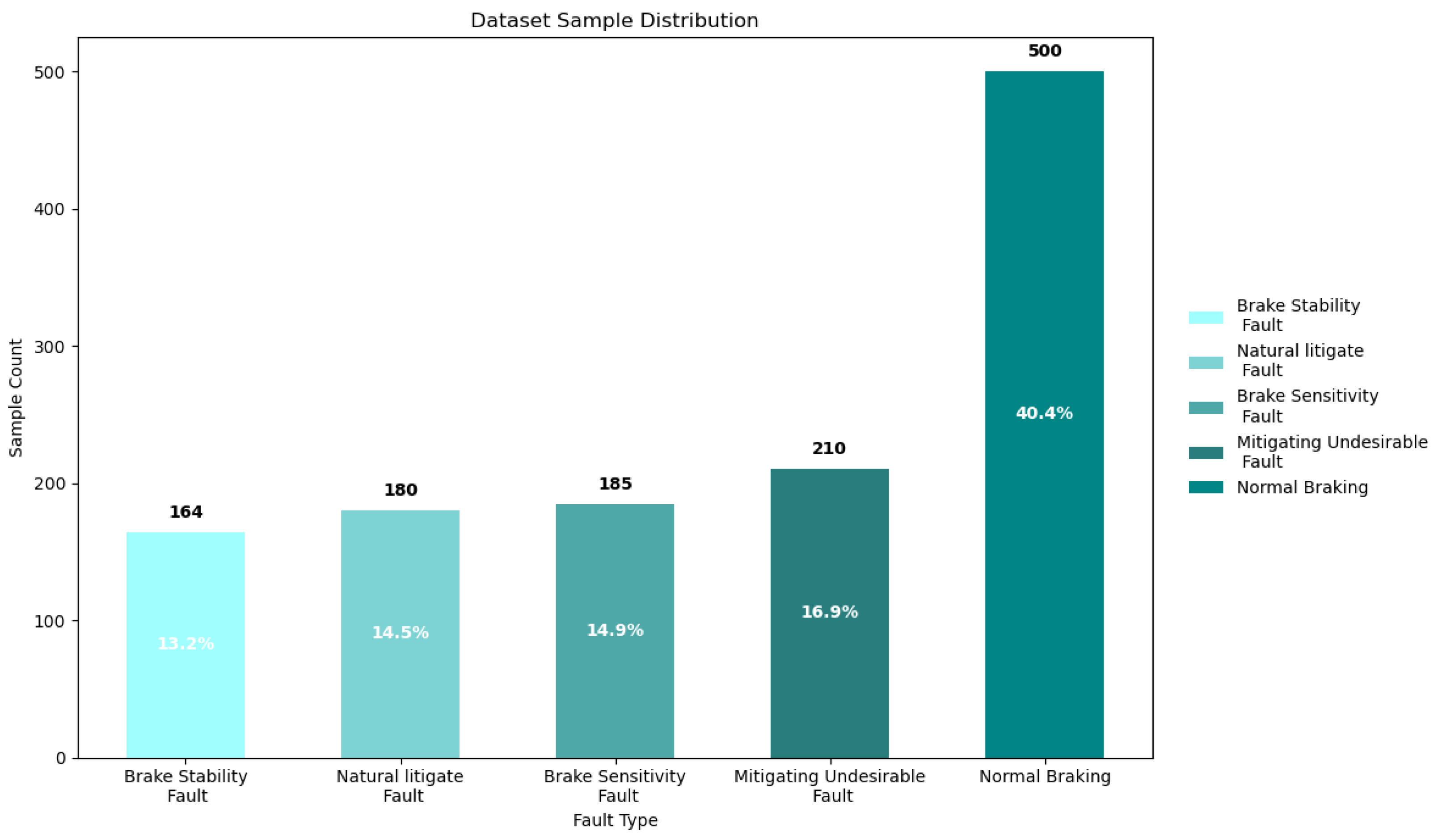
The braking data utilized in this study is collected from the communication between the CCU and the ATP system of heavy-haul railway freight vehicles. A total of 1239 braking instances were recorded, corresponding to 1239 images of train braking curves with dimensions of 265 × 187 × 3. The dataset was randomly divided into training and testing sets at a ratio of 5:1. Based on the types of braking system faults, the data is categorized into five classes: normal braking, brake sensitivity fault, mitigating undesirable fault, brake stability fault, and natural mitigate fault. As shown in Figure 6, we use class weighting to address the class imbalance issue of fault samples.
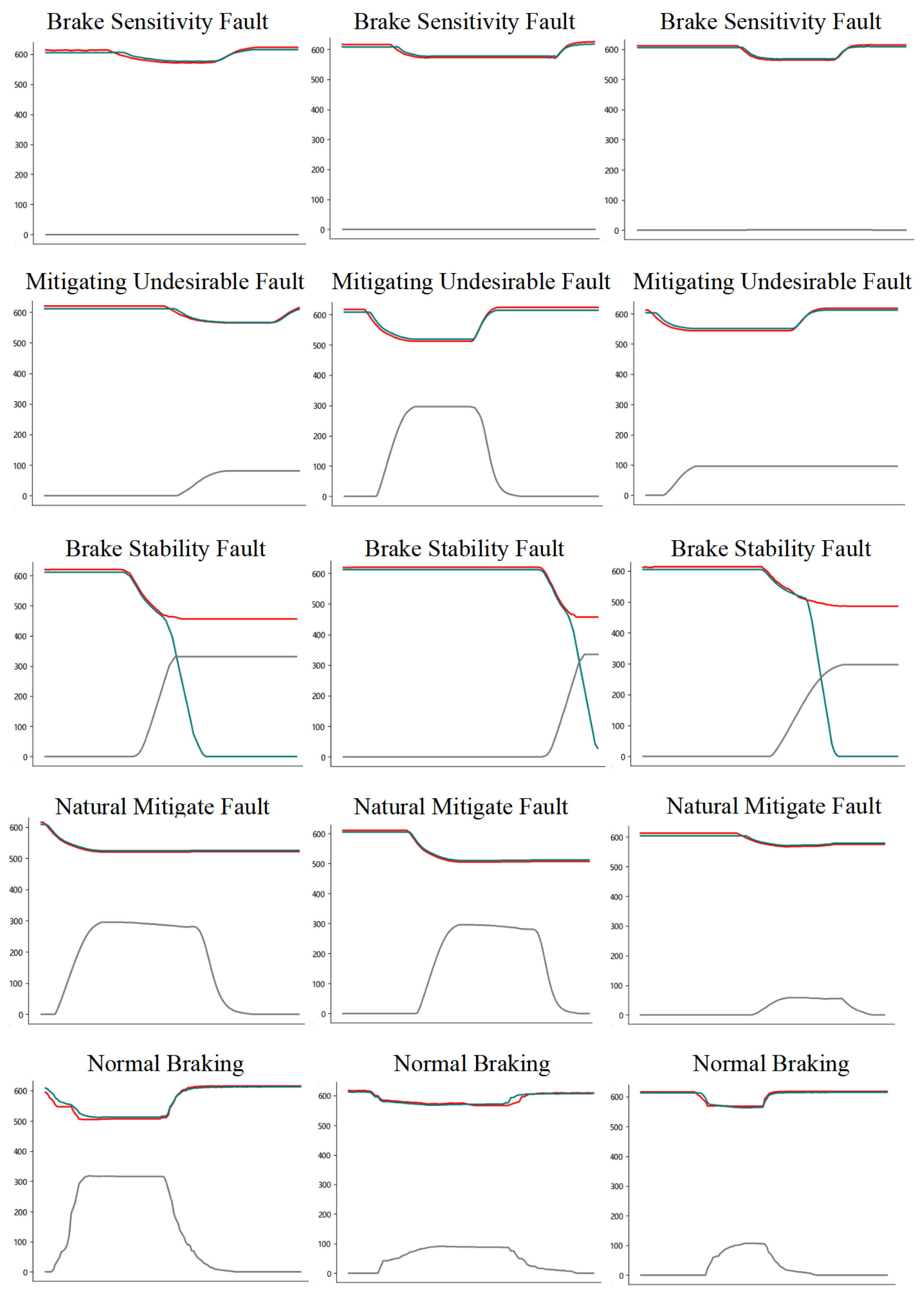
To enhance the classification of train braking faults, braking curve images were collected under conditions of minimum braking force, normal braking, and maximum braking force. Additionally, since the number of coupled vehicles can influence the braking curve images, data was also gathered for single locomotive operation, as well as for 10-vehicle and 20-vehicle coupled configurations. A subset of the train braking curve dataset is illustrated in Figure 7. The y-axis represents pressure (kPa) and the x-axis represents time (s). The red curve denotes the Auxiliary Reservoir Pressure, the green curve denotes the Train Pipe Pressure, and the gray curve denotes the Brake Cylinder Pressure.

4.3. Parameter Configuration

In the experiment for diagnosing faults in the train braking system, to validate the performance advantages of the CARE model, the parameters of the three models—CR, CAR, and CARE—were configured to be largely consistent. The parameter settings for these models are detailed in Table 1.

4.4. Analysis of Experimental Results

1. Comparison of Model Accuracy
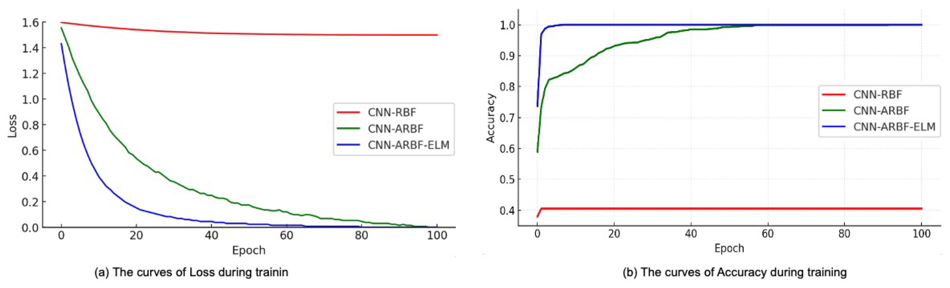
We employed three distinct models, which are the fundamental CR, the adaptive CAR, and the optimized CARE to train on image data of the braking process. Following 100 iterations of training, the variations in loss values and accuracy on the training set are depicted in Figure 8a and Figure 8b, respectively.
After 50 iterations, the CR model exhibited minimal changes in loss values, achieving an accuracy of only 40.32%. This indicates that the CR model had converged and reached a local optimum, leading to overfitting of the data. In contrast, the CAR model demonstrated improved performance. After 80 iterations, the loss values stabilized at a lower level compared to the CR, and the CAR model achieved convergence with superior fitting results. By the 100th iteration, the accuracy reached 98.49%, demonstrating that the CAR model effectively addressed the overfitting issues inherent in the CR model. Furthermore, the CARE model, which was optimized by increasing the number of neural network layers and incorporating the ELM algorithm, showed even more promising results. After just 40 iterations, the loss values began to converge, approaching zero, and the model achieved 100% accuracy within approximately 10 iterations. This highlights the exceptional fitting performance of the CARE model.
2. Comparison of Model Reliability
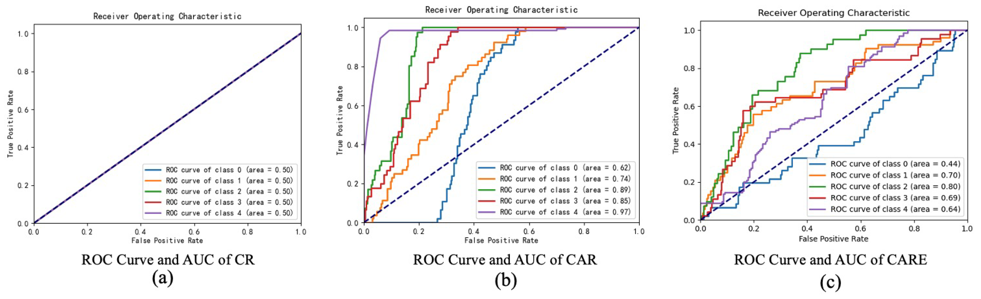
The ROC curve and AUC values for the classification results of the CR model on the test dataset are illustrated in Figure 9a. During the training process, the model became trapped in a local optimum, resulting in AUC values of 0.5 for all five data types, rendering it practically unusable in real-world applications. In contrast, the ROC curve and AUC values for the CAR model, as shown in Figure 9b, demonstrate significant improvement. The adaptive CAR model achieved AUC values greater than 0.5 for each braking curve classification, indicating its enhanced capability to identify four types of faults. The average AUC value for these four fault types reached 0.8625. However, the AUC value for normal braking was only 0.62, suggesting a tendency to misclassify normal braking as faults. The ROC curve and AUC values for the CARE model, depicted in Figure 9c, exhibit remarkable performance. The ROC curve is positioned close to the top-left corner, and the average AUC value reached 0.994, highlighting the superior fitting capability of the CARE model.
3. Comparison of CARE with Other Models
To further validate the proposed model efficacy, this research compared the CARE model with three other fault diagnosis models: PCA-HMM [25], PCA-GA-SVM [26], and CNN-GRU [27], focusing on feature dimension, number of layers, training time, accuracy, and F1-score. As shown in Table 2, when handling high-dimensional datasets, the CARE architecture achieves significantly reduced per-epoch training duration, completing each cycle in merely 1.048 s on average. This represents a 48.8% time reduction compared to the PCA-HMM (previously the fastest training baseline) model and a 2.71% accuracy improvement over PCA-GA-SVM (the prior precision leader). In addition, the F1-score of the model reaches 96.30%, significantly outperforming other comparative models. Compared to modern deep models such as CNN-ResNet and Transformer, CNN-ARBF-ELM not only achieves superior accuracy but also demonstrates greater engineering application value in terms of training efficiency. Experimental findings substantiate the superior diagnostic capability and enhanced generalization performance of the proposed CARE hybrid framework for railway braking system fault identification.

5. Conclusions

In this study, leveraging the superior real-time state feature extraction capability of RBF networks, we introduce the K-Means clustering algorithm to adaptively construct RBF centers and optimize their radii. Simultaneously, the ELM algorithm is employed to optimize the subsequent layers added after the ARBF network. Ultimately, we construct a CARE model for real-time fault diagnosis of four braking system faults, including brake sensitivity faults, mitigating undesirable fault, brake stability faults, and natural mitigate faults. In the future research, we will focus on extending this model to broader domains, continuously refining it through practical implementation to provide robust technical support for enhancing both safety and economic efficiency in railway transportation.

Author Contributions

Conceptualization, Y.B. and H.L.; Methodology, Y.B. and G.G.; Data curation, Y.B., G.G. and Y.X.; Writing—original draft, Y.B.; writing—review and editing, Y.B. and H.L.; Supervision, N.S.; Funding acquisition, H.L. All authors have read and agreed to the published version of the manuscript.

Funding

This research was funded by the Scientific and Technological Development Program Project of China State Railway Group Co., Ltd. (Grant No. P2023T002), and the Scientific and Technological Innovation Project of China National Energy Co., Ltd. (Grant No. SHGF-17-56).

Data Availability Statement

The dataset presented in this study consists of China Energy Group brake data of freight cars, covering the period from 1 January 2022 to 30 December 2023. Due to ownership restrictions imposed by the third-party organization, the dataset is not publicly accessible at this time. However, despite these restrictions, we remain committed to collaborating with researchers and students who seek access to the dataset for academic and research purposes. Researchers with a legitimate academic or professional interest in the dataset may contact the Information Technology Department of the China Energy Group to inquire about potential access. For further inquiries, please reach out via email at 11591129@ceic.com.

Conflicts of Interest

The authors declare that this study received funding from China National Railway Group Corporation Limited (Grant No. 2319YF8501). The funder was not involved in the study design, collection, analysis, interpretation of data, the writing of this article or the decision to submit it for publication.

References

  1. Montenegro, P.A.; Carvalho, H.; Ribeiro, D. Assessment of train running safety on bridges: A literature review. Eng. Struct. 2021, 241, 112425. [Google Scholar] [CrossRef]
  2. Li, H.; Wang, H.; Xu, Z. Fault diagnosis of railway freight car wheelset based on deep belief network and cuckoo search algorithm. Proc. Inst. Mech. Eng. Part F 2022, 5, 501–510. [Google Scholar] [CrossRef]
  3. Du, Y.; Li, H.; He, M. A BiGRU autoencoder remaining useful life prediction scheme with attention mechanism and skip connection. IEEE Sens. J. 2021, 21, 10905–10914. [Google Scholar]
  4. Zio, E. Prognostics and Health Management (PHM): Where are we and where do we (need to) go in theory and practice. Reliab. Eng. Syst. Saf. 2022, 218, 108119. [Google Scholar] [CrossRef]
  5. Zhang, X.; Chen, S.; Yang, T. Research on the air brake system of heavy haul trains based on neural network. Veh. Syst. Dyn. 2024, 62, 2035–2053. [Google Scholar]
  6. Du, Y.; Li, Z.; Li, H. A hybrid-driven remaining useful life prediction method combining asymmetric dual-channel autoencoder and nonlinear Wiener process. Appl. Intell. 2023, 53, 25490–25510. [Google Scholar]
  7. Wang, Q.; Cole, C.; Szymkat, M. Freight train air brake models. Int. J. Rail Transp. 2023, 11, 1–49. [Google Scholar]
  8. Guo, X.; Chen, Q.; Liu, L. An approach for simulating the air brake system of long freight trains based on fluid dynamics. Railw. Eng. Sci. 2023, 31, 122–134. [Google Scholar]
  9. Pérez Hernández, M.; Montes Rivera, M.; Pérez Hernández, R. Diagnosis of the Car Brake System with Fuzzy-Bayesian Expert System. Int. J. Comb. Optim. Probl. Inform. 2024, 15, 26. [Google Scholar] [CrossRef]
  10. Chen, B.; Xu, M.; Liu, Y. Availability-based engineering resilience metric and its corresponding evaluation methodology. Reliab. Eng. Syst. Saf. 2018, 172, 216–224. [Google Scholar] [CrossRef]
  11. Li, M.; Huang, P.; Fan, Y. Development of compound fault diagnosis system for gearbox based on convolutional neural network. Sensors 2020, 20, 6169. [Google Scholar] [CrossRef]
  12. Chen, H.; Ma, W.; Liu, Y.; Qiao, Q. An anti-noise fault diagnosis approach for rolling bearings based on multiscale CNN-LSTM and a deep residual learning model. Meas. Sci. Technol. 2023, 34, 045013. [Google Scholar] [CrossRef]
  13. Zhang, Y.; Zhang, T.; Huang, X. Fault diagnosis of rotating machinery based on recurrent neural networks. Measurement 2021, 171, 108774. [Google Scholar] [CrossRef]
  14. Wang, P. The application of radial basis function (RBF) neural network for mechanical fault diagnosis of gearbox. IOP Conf. Ser. Mater. Sci. Eng. 2017, 269, 012056. [Google Scholar] [CrossRef]
  15. Wang, J.; Zhang, S.; Hu, X. A fault diagnosis method for lithium-ion battery packs using improved RBF neural network. Front. Energy Res. 2021, 9, 702139. [Google Scholar] [CrossRef]
  16. Gao, W.; Huang, Z.; Yang, J. Intelligent monitoring system for braking performance of heavy haul railway freight cars. In Proceedings of the IEEE International Academic Exchange Conference on Science and Technology Innovation (IAECST), Guangzhou, China, 10–12 December 2021; Volume 3, pp. 1334–1340. [Google Scholar]
  17. Abdel-Nasser, S. Principle of neural network and its main types. J. Adv. Appl. Comput. Math. 2020, 7, 8–19. [Google Scholar] [CrossRef]
  18. Kowalski, W.; Stasiak, P.; Strumillo, P. Kernel orthonormalization in radial basis function neural networks. IEEE Trans. Neural Netw. 1997, 8, 1177–1183. [Google Scholar]
  19. Kittipong, S.; Phetthong, P.; Sritrakool, N. Generalized multiquadratic radial basis function neural networks (RBFNNs) with variable shape parameters for function recovery. In Proceedings of the Fuzzy Systems and Data Mining, Virtual Event, 26–29 October 2021; Volume VII, pp. 77–85. [Google Scholar]
  20. He, S.; Chen, Q.; Han, M. Parameter selection in SVM with RBF kernel function. In Proceedings of the IEEE World Automation Congress, Puerto Vallarta, Mexico, 24–28 June 2012; pp. 1–4. [Google Scholar]
  21. Park, B.J.; Pedrycz, W.; Oh, S.K. Polynomial-based radial basis function neural networks (P-RBF NNs) and their application to pattern classification. Appl. Intell. 2010, 32, 27–46. [Google Scholar] [CrossRef]
  22. Yang, Z.; Yang, J.; Liu, M. A Method for Predicting Trajectories of Concealed Targets via a Hybrid Decomposition and State Prediction Framework. Sensors 2025, 25, 3639. [Google Scholar] [CrossRef]
  23. Yu, H.; Zhang, Y.; Zhang, Y. Drivers’ visual interaction performance of on-board computer under different heat conditions: Based on ELM and entropy weight. Sustain. Cities Soc. 2022, 81, 103835. [Google Scholar] [CrossRef]
  24. Li, X.; Su, K. Implementation of Deep Pose Estimator Based Emotion Recognition System. In Proceedings of the IEEE International Automatic Control Conference, Penghu, Taiwan, 21–23 May 2023; pp. 1–6. [Google Scholar]
  25. Usman, A.M. On Eigendecomposition Based Algorithms as Feature Extraction Techniques Used with Hidden Markov Model for the Detection of Whale Vocalisations. 2024. Available online: https://ee.sun.ac.za/on-eigendecomposition-based-algorithms-as-feature-extraction-techniques-used-with-hidden-markov-model-for-the-detection-of-whale-vocalisations/ (accessed on 9 February 2026).
  26. Yang, T.; Xu, Y.; Zhang, H. Insulation fault diagnosis of disconnecting switches based on wavelet packet transform and PCA-IPSO-SVM of electric fields. IEEE Access 2020, 8, 176676–176690. [Google Scholar]
  27. Kumar, R.; Anand, R.S. A deep learning-based CNN-GRU prediction model for early fault diagnosis in rolling ball bearings. Neural Comput. Appl. 2025, 37, 17015–17030. [Google Scholar] [CrossRef]
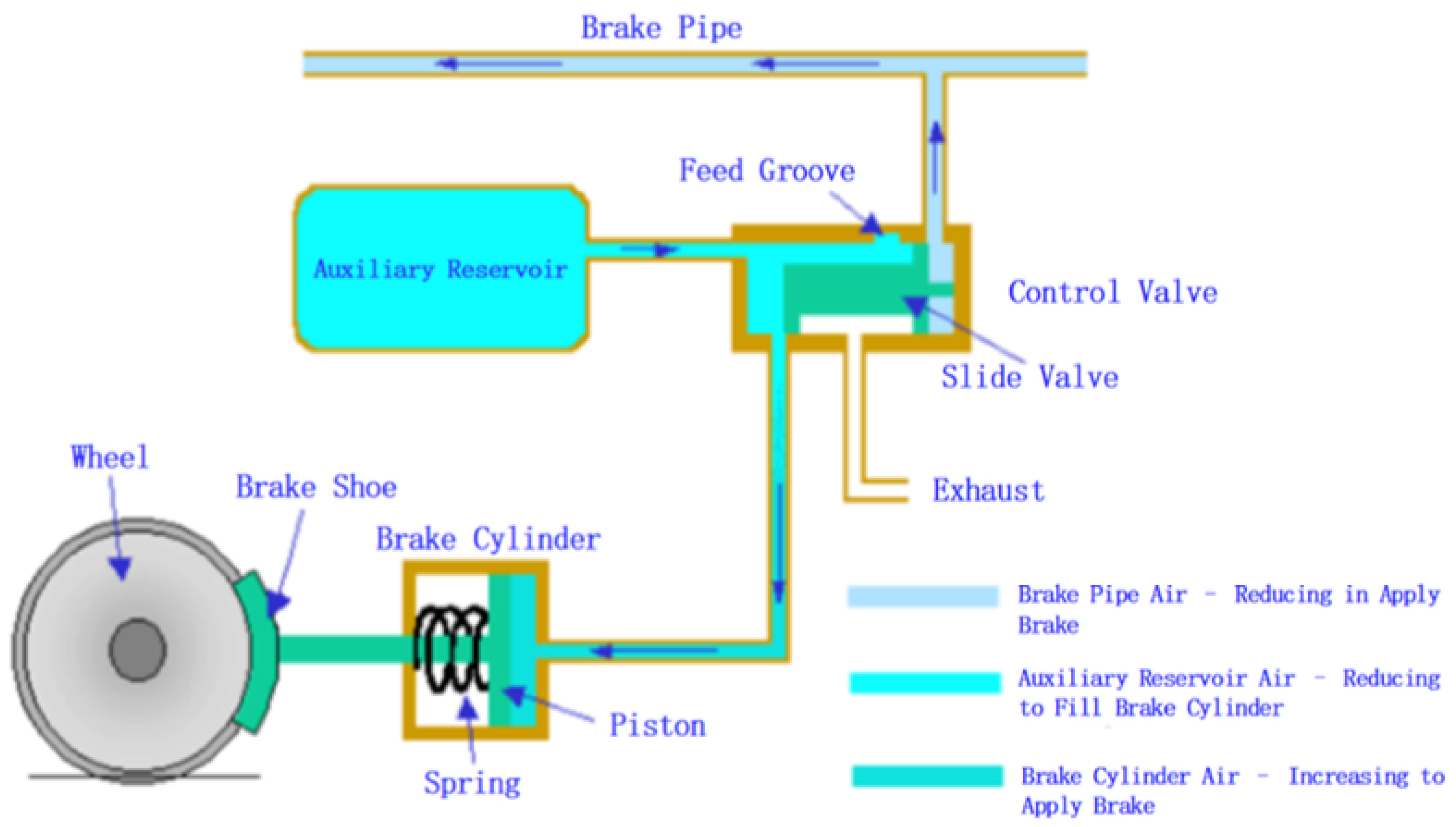
Figure 1. Schematic diagram of the train braking system.
Electronics 15 00895 g001
Figure 2. Train Braking System Fault Classification.
Electronics 15 00895 g002
Figure 3. CNN basic structure.
Electronics 15 00895 g003
Figure 4. Structure of the ELM network.
Electronics 15 00895 g004
Figure 5. Fault diagnosis model construction.
Electronics 15 00895 g005
Figure 6. Dataset Sample Distribution.
Electronics 15 00895 g006
Figure 7. Visualization of a Train Braking Curve Dataset Subset (Normal State and Four Fault States).
Electronics 15 00895 g007
Figure 8. The curves of Loss and Accuracy during training.
Electronics 15 00895 g008
Figure 9. ROC curve and AUC value.
Electronics 15 00895 g009
Table 1. Model training parameters.
Model NameNumber of
Layers
Optimization
Algorithm
IterationsBatch
Size
Data
Dimension
CR8Adam10064 265 × 187 × 3
CAR8Adam10064 265 × 187 × 3
CARE9Adam10064 265 × 187 × 3
Table 2. Comparison of different models.
ModelFeature DimensionNo. of LayersTraining Time (s)Acc (%)F1-Score (%)
PCA-HMM [23]422.03890.2089.75
PCA-GA-SVM [24]435.04496.7793.10
CNN-GRU [25] 192 × 144 × 3 72.06995.0094.35
CNN-ResNet 224 × 224 × 3 102.51297.0092.60
Transformer12863.20096.2094.90
CNN-ARBF-ELM 265 × 187 × 3 91.04899.4096.30
Disclaimer/Publisher’s Note: The statements, opinions and data contained in all publications are solely those of the individual author(s) and contributor(s) and not of MDPI and/or the editor(s). MDPI and/or the editor(s) disclaim responsibility for any injury to people or property resulting from any ideas, methods, instructions or products referred to in the content.