Graph Neural Networks for City-Scale Electric Vehicle Charging Demand and Road-Network Flow Forecasting: Empirical Ablations on Graph Structure and Exogenous Features

Abstract

City-scale forecasting is essential for both electric-vehicle (EV) charging operations (e.g., peak management and resource allocation) and urban mobility management (e.g., road-network flow monitoring and incident response). Spatio-temporal graph neural networks (STGNNs) are a natural candidate for these problems, yet their performance often critically depends on the choice of a predefined graph prior and the availability/quality of exogenous signals. Importantly, we do not intentionally construct a poor graph; rather, we treat any predefined adjacency as a testable hypothesis and verify its alignment with the forecasting target via no-graph ablations and lightweight diagnostics ($\Delta corr$, $E_D$). In this work, we present a unified experimental pipeline based on a spatio-temporal graph convolutional network (STGCN) backbone and conduct systematic ablations on (i) whether and how a predefined static graph is used and (ii) how feature sets influence multi-step forecasting accuracy. We evaluate on two city-scale hourly datasets with heterogeneous node counts (UrbanEV: 275 nodes; CHARGED-AMS_remove_zero: 1388 nodes) and a 24 h input/6 h output setting. Across datasets, we find that a static graph can be beneficial only when it matches the true dependency structure; otherwise, it may degrade accuracy substantially. On UrbanEV, removing the graph component improves overall MAE from 116.21 ± 5.43 to 66.53 ± 1.71 (S = 5 seeds, 0–4), outperforming a persistence baseline (MAE 94.16). Feature ablations further analyze how occupancy and price signals affect UrbanEV accuracy (e.g., MAE 87.32 with all features under the evaluated feature setting). On CHARGED, the volume-only setting performs best among tested feature combinations (MAE 0.127), closely tracking a persistence baseline (MAE 0.139), while additional covariates may introduce noise under static modeling. We provide detailed multi-horizon results and discuss practical implications for when graph priors help or hurt in real deployments.

1. Introduction

The rapid electrification of transportation is reshaping both energy and mobility systems worldwide. As electric vehicles (EVs) proliferate, city-scale EV charging infrastructure faces the challenge of accommodating highly variable demand patterns, which are influenced by factors such as user behavior, daily routines, and external events. Effective forecasting of charging demand is crucial for operational tasks like peak load management, dynamic resource allocation, and ensuring grid stability without overprovisioning infrastructure. Similarly, in urban mobility systems, accurate forecasting of road-network flows is indispensable for traffic management, congestion mitigation, incident response, and long-term urban planning. These two domains—EV charging and road traffic—share fundamental similarities: they involve spatially distributed entities (e.g., charging stations or road sensors), exhibit strong temporal autocorrelations due to periodic human activities, and feature complex spatial interactions arising from network topology, behavioral patterns, and exogenous variables like weather or pricing policies.

Beyond operational efficiency, these forecasts are increasingly used as inputs to urban sustainability analytics, e.g., estimating congestion-related emissions, evaluating electrification benefits, and planning mitigation actions. While transport electrification reduces tailpipe emissions, many cities will remain in a mixed-fleet regime for years; hence complementary emissions-control technologies (after-treatment systems and advanced filtration) are still actively studied. Recent work on compact Nomex/activated-carbon filtration with IoT-based monitoring for gasoline-engine exhaust illustrates the role of materials and filtration technologies as a representative emissions-mitigation direction [1].

Deep learning models tailored for spatio-temporal data have emerged as powerful tools for addressing these forecasting challenges. In particular, spatio-temporal graph neural networks (STGNNs) have gained prominence in traffic forecasting [2,3,4] and are increasingly applied to EV charging prediction tasks [5]. STGNNs leverage graph structures to model spatial dependencies, such as adjacency in road networks or proximity between charging stations, while incorporating temporal modeling components like convolutions or recurrences to capture time-series dynamics. This hybrid approach allows STGNNs to propagate information across both space and time, potentially leading to more accurate predictions in networked systems. However, the efficacy of STGNNs in real-world deployments hinges on critical assumptions: the predefined graph must accurately reflect underlying dependencies, and exogenous features must provide meaningful signals without introducing undue noise or complexity.

Despite the widespread adoption of STGNNs, a key practical question remains underexplored in many application-oriented studies: under what conditions does incorporating a predefined static graph enhance forecasting performance, and when might it inadvertently degrade it? Static graphs, often constructed based on geographic proximity (e.g., k-nearest neighbors) or known topologies, may not align with actual functional relationships, such as demand substitution between competing stations or dynamic rerouting in traffic flows. Mismatched graphs can lead to spurious correlations, oversmoothing of node-specific signals, or propagation of irrelevant information, ultimately harming multi-step forecast accuracy. Furthermore, the inclusion of exogenous features, such as session duration, occupancy rates, or pricing signals, adds another layer of complexity; while these can enrich the model’s input, they may also amplify noise if their predictive value is weak or varies across contexts. This concern is closely related to the emerging literature on heterophilic graph learning, which emphasizes that message passing over a static topology is not universally beneficial when neighboring nodes are not “compatible” in terms of feature/structural similarity. In such cases, graph-based aggregation can systematically mix dissimilar signals and deteriorate the predictive performance, motivating diagnostics that verify whether a predefined graph is aligned with the dependency structure of the forecasting target.

This paper addresses these gaps through a rigorous empirical investigation, employing systematic ablations within a unified forecasting pipeline built on an STGCN backbone [2]. We focus on ablating (i) the use of graph structure, by comparing models with and without spatial mixing, and (ii) feature sets, by progressively incorporating exogenous signals. Our experiments are conducted on two real-world city-scale datasets with differing scales and characteristics, using a standardized 24 h input and 6 h output horizon to simulate operational scenarios. By maintaining a consistent model architecture and evaluation protocol, we isolate the impacts of these design choices and provide reproducible insights for practitioners.

Contributions. (1) We unify city-scale EV charging demand and road-network flow forecasting under the same multi-step STGNN framework, highlighting shared modeling challenges and opportunities. (2) We conduct systematic graph-usage ablations (with-graph vs. no-graph) and feature ablations on two datasets with different node scales and covariates, revealing when graphs help or hinder. (3) We report detailed horizon-wise metrics and analyze failure modes of static graph priors, offering actionable guidance for smart-city deployments. These findings underscore the need for empirical validation of modeling assumptions in applied STGNN research.

Scope clarification. This paper studies two closely related city-scale forecasting tasks, EV charging demand forecasting and road-network flow forecasting, under a unified multi-step STGCN-based pipeline. We use UrbanEV as a road-network flow benchmark and CHARGED as an EV charging demand benchmark to examine when a predefined static graph prior and exogenous features help or hurt under consistent model capacity and evaluation protocol. The methodological insights and diagnostics developed here are applicable to a broad range of urban spatio-temporal signals.

2. Related Work

2.1. Traffic Flow Forecasting with Spatio-Temporal Graph Models

Traffic flow forecasting has a rich history, evolving from traditional statistical methods to advanced deep learning techniques that explicitly account for spatial dependencies. Early approaches relied on road topology or sensor proximity to encode spatial relationships, often using autoregressive integrated moving average (ARIMA) models or Kalman filters for temporal prediction. Modern deep learning paradigms have shifted toward more sophisticated architectures, including diffusion-based recurrent models like DCRNN [3], which propagate information through graph diffusion convolutions; temporal convolutional networks that capture multi-scale patterns; and attention-based models such as GMAN [6], which dynamically weigh spatial and temporal interactions.

At the forefront are STGNNs, which integrate graph convolutions for spatial modeling with temporal modules like gated recurrent units or convolutions. Key representatives include STGCN [2], which combines graph and temporal convolutions for efficient computation; Graph WaveNet [4], which introduces adaptive adjacency learning alongside dilated convolutions; and advanced variants like MTGNN [7] and AGCRN [8], which learn node embeddings or adjacency matrices end-to-end to adapt to data-driven dependencies. These models have demonstrated superior performance on benchmark datasets such as METR-LA and PEMS-BAY, often outperforming non-graph baselines by leveraging spatial priors.

However, the practical utility of graph priors is not always guaranteed. In operational environments, sensor dependencies may arise from dynamic factors like route choices, demand shifts, or traffic control policies, rather than static geometric proximity. This discrepancy can lead to suboptimal performance if the graph introduces misleading aggregations. Consequently, ablation studies are essential to verify whether a given graph enhances the predictions beyond what purely temporal models (e.g., ARIMA or simple LSTMs) can achieve, motivating our controlled comparisons in this work.

2.2. EV Charging Demand Forecasting

Forecasting EV charging demand encompasses a range of granularities, from individual station-level predictions to aggregated city-wide estimates. Traditional methods include statistical techniques like regression models or time-series decomposition, while deep learning has introduced recurrent networks (e.g., LSTMs) for capturing sequential patterns and transformers for handling long-range dependencies [9,10,11,12,13]. Graph-based approaches are gaining traction where spatial coupling is evident, such as in networks of charging stations, where demand at one location influences others nearby due to user preferences or infrastructure constraints [5].

Exogenous signals play a pivotal role in enhancing accuracy; for instance, pricing (electricity or service fees), occupancy rates, and session durations can signal upcoming demand fluctuations, but their integration requires careful consideration. If these features exhibit weak or nonstationary relationships with the target (e.g., volume), they may introduce noise, particularly in static models without adaptive mechanisms. Public datasets, such as multi-city charging records or high-resolution station data [14], have facilitated more standardized evaluations, enabling comparisons across methods.

Despite these advances, few studies provide reproducible ablations quantifying the marginal benefits of graph structures over temporal-only modeling in EV contexts. Our work fills this void by systematically evaluating graph and feature contributions on real datasets, drawing parallels to traffic forecasting to underscore cross-domain insights.

2.3. Graph Construction and When Graphs Hurt

Graph construction in spatio-temporal graph neural networks (STGNNs) typically follows predefined strategies such as distance-based k-nearest-neighbor (kNN) graphs for spatial proximity, correlation-based graphs for empirical dependencies, or topology-derived graphs for known networks (e.g., road links). While effective in controlled settings, these static approaches implicitly assume stable relationships over time, which may not hold in dynamic systems influenced by user behavior, external policies, or nonstationary demand patterns.

To mitigate this limitation, adaptive graph learning techniques [4,7,8] infer adjacency matrices or node embeddings during training, offering greater flexibility at the cost of additional parameters and potential overfitting. These approaches typically require careful regularization and validation to ensure generalization. An underutilized yet practical diagnostic is benchmarking against a “no-graph” ablation, where the adjacency matrix is set to the identity matrix, effectively removing cross-node message passing while preserving the temporal backbone and overall architecture. This isolates the contribution of spatial mixing and reveals cases where graph usage degrades performance due to mismatch or oversmoothing.

Beyond the conventional “graphs help by proximity” narrative, heterophilic graph learning provides a principled lens to understand when static graphs may hurt. Recent studies argue that homophily should be disentangled into multiple aspects (e.g., feature and structural alignment), and that standard neighborhood aggregation can fail when the graph links nodes whose signals are weakly related or not mutually informative. Comprehensive summaries and benchmarks are available in the heterophilic graph learning handbook [15], while work on disentangling graph homophily further highlights that simplistic homophily measures are insufficient to predict GNN behavior [16]. Moreover, heterophily considerations extend to temporal settings: recent temporal heterophilic graph models explicitly study heterophily in event-based or dynamic graphs and propose dedicated measurements and filters [17]. These developments are highly relevant to forecasting deployments, where practitioners often rely on a fixed convenient topology (e.g., distance-based or administratively defined adjacency) that may not match the true dependency structure of the target process.

Our study employs this ablation strategy to empirically assess graph utility, complementing prior work on adaptive methods. For future extensions, recent transformer-based spatio-temporal models such as PatchTST [12] and TimesNet [13] can serve as strong non-graph alternatives, while dynamic-graph forecasting models (e.g., DGCRN [18]) may better capture time-varying dependencies when a fixed topology is insufficient.

3. Materials and Methods

3.1. Problem Formulation

We formalize the spatio-temporal forecasting problem as follows. Let $X\in {\mathbb{R}}^{T\times N\times F}$ represent a multivariate spatio-temporal tensor, where $T$ is the number of time steps, $N$ is the number of nodes (e.g., charging stations or road sensors), and $F$ is the number of features per node–time pair. The goal is to learn a parameterized function $f_{\theta }$ that, given an input window of length $L$, predicts the target variable over the next $H$ time steps: ${\widehat{Y}}_{t:t+H-1}=f_{\theta }\left(X_{t-L+1:t}\right)$, where $\widehat{Y}\in {\mathbb{R}}^{H\times N}$ denotes the predicted values (e.g., charging volume or traffic flow) for each node.

In this study, we adopt a multi-step direct forecasting strategy, where all $H$ future steps are predicted in a single forward pass, avoiding error accumulation from iterative methods. We set $L=24$ (one day) and $H=6$ (six hours) to align with practical horizons for day-ahead planning and short-term operations in EV charging and traffic management.

3.2. Datasets and Features

To evaluate our ablations, we use two city-scale datasets with hourly resolution that differ in node density, task focus, and feature availability.

The UrbanEV dataset comprises 275 nodes and 4344 hourly time steps, covering the period from 1 September 2022 00:00 to 28 February 2023 23:00. It targets road-network flow forecasting and includes traffic-related signals such as volume (primary target), duration, and occupancy, alongside price-related covariates (electricity price $e_{price}$, service price $s_{price}$) and temporal encodings (e.g., sine/cosine representations of hour-of-day and day-of-week). After preprocessing, this yields 9 input channels. Raw observations are aggregated to hourly bins; missing entries are represented as NaN and accompanied by a binary observation mask. During min–max normalization, NaNs are ignored when computing feature-wise minima/maxima and are filled with zeros only after normalization for tensor input, while the mask is used to exclude missing targets from training loss and evaluation metrics.

The CHARGED-AMS_remove_zero dataset, focused on EV charging demand forecasting, features 1388 nodes and 4392 hourly time steps from 1 April 2023 00:00 to 30 September 2023 23:00 [14]. It provides the charging volume (target) and duration per node, electricity and service price covariates ($e_{price}$, $s_{price}$), and similar temporal encodings, resulting in 8 channels. Preprocessing mirrors UrbanEV, with zero-volume entries removed as per the dataset variant and missing entries represented as NaN with a binary observation mask that is propagated through training and evaluation.

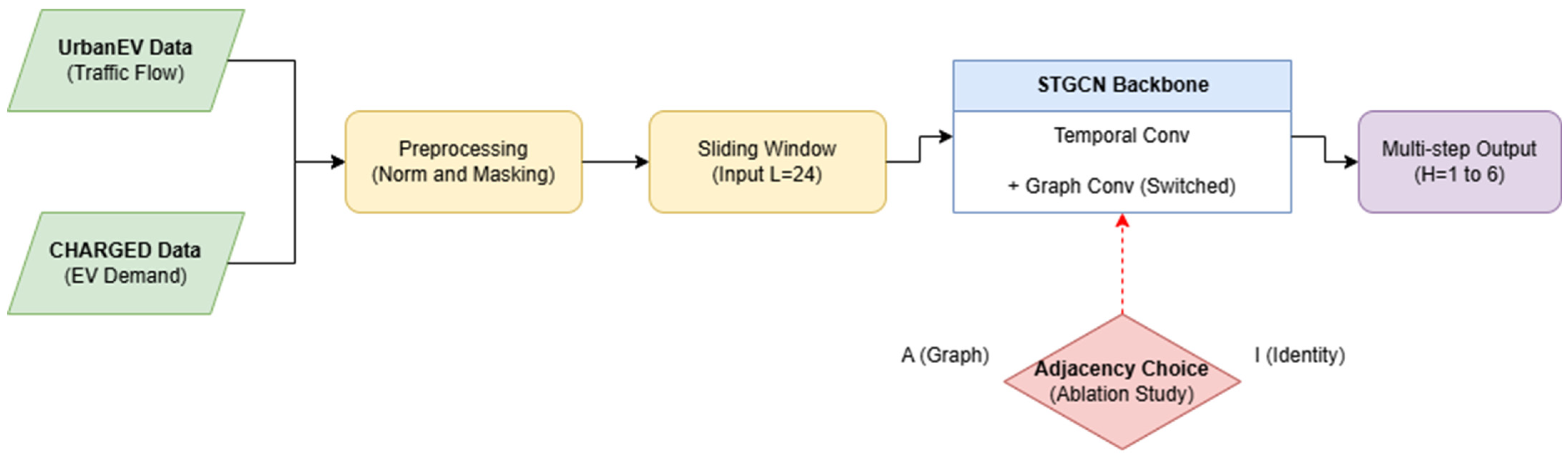
For both datasets, we apply consistent preprocessing: (i) feature-wise min–max normalization computed on the training split; (ii) periodic time encodings; and (iii) sliding-window extraction for input–output pairs. We carry a binary observation mask M where $M_{\left\{t,i\right\}}=1$ if the target at node i and time t is observed and 0 otherwise, ensuring missing targets do not contribute to training loss or evaluation metrics. In the raw files or intermediate storage, missing entries may be encoded using a sentinel value (e.g., −1). In preprocessing, we immediately convert such sentinels to NaN before fitting the scaler. During min–max normalization, NaNs are ignored when computing feature-wise minima/maxima and are filled with zeros only after normalization for tensor input, while the mask is used throughout training and evaluation. This design ensures the sentinel never interacts with normalization or masking. The overall pipeline for multi-step city-scale forecasting is illustrated in Figure 1.

Predefined static graphs. We consider commonly used predefined static graphs that encode spatial proximity as a convenient structural prior. For CHARGED, we build a distance-based k-nearest-neighbor (kNN) graph using the provided pairwise distance matrix. Specifically, for each node $i$, we connect it to its $k$ nearest neighbors ($k=8$), symmetrize the edge set, and assign Gaussian edge weights.

$$w_{ij}=\exp \left(-{\displaystyle \frac{d_{ij}^2}{{\sigma }^2+\epsilon }}\right),$$

where $d_{ij}$ denotes the distance between nodes $i$ and $j$, $\epsilon$ is a small constant for numerical stability, and $\sigma$ is set to the median of $\left\{d_{ij}\right\}$ over the selected edges. For UrbanEV, we directly use the dataset-provided adjacency matrix as the predefined static graph prior. For all predefined graphs, we add self-loops and apply symmetric normalization before feeding the graph into STGCN:

$$\widehat{\mathrm{A}}={\mathrm{D}}^{-{\displaystyle \frac{1}{2}}}\left(\mathrm{A}+\mathrm{I}\right){\mathrm{D}}^{-{\displaystyle \frac{1}{2}}},$$

where $\mathrm{D}$ is the degree matrix of $(\mathrm{A}+\mathrm{I})$.

3.3. Model Backbone: STGCN with Optional Graph

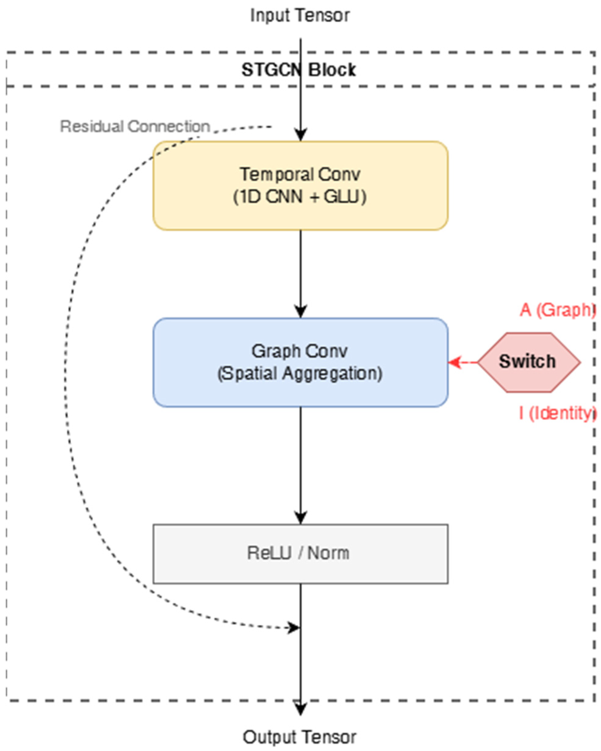
Our experimental pipeline centers on a spatio-temporal graph convolutional network (STGCN) backbone [2], selected for its balance between efficiency and expressive power in multivariate spatio-temporal forecasting. The backbone is composed of stacked spatio-temporal blocks with residual connections to stabilize optimization. Each block applies a temporal convolution to capture local temporal dynamics, followed by a graph convolution to optionally mix information across nodes according to a specified adjacency matrix. The STGCN block and the no-graph switch (A vs. I) are illustrated in Figure 2.

Let the block input be $Z\in {\mathbb{R}}^{T^{\prime }\times N\times C}$, where $T^{\prime }$ is the (possibly reduced) temporal length at the current stage, $N$ is the number of nodes, and $C$ is the channel dimension. The temporal module performs a 1D convolution along the time axis with kernel size 3:

$$Z^{\prime }=Conv1D\left(Z\right).$$

The spatial module then performs graph convolution using an adjacency matrix $A\in {\mathbb{R}}^{N\times N}$,where $W$ is a learnable weight matrix, $\sigma \left(\cdot \right)$ is a point-wise nonlinearity (e.g., ReLU), and $\tilde{A}$ denotes the symmetrically normalized adjacency:

$$\tilde{A}=D^{-{\displaystyle \frac{1}{2}}}A{D}^{-{\displaystyle \frac{1}{2}}},D_{ii}=\sum _j{A}_{ij}.$$

Unless otherwise noted, we use two spatio-temporal blocks with hidden dimension 32.

Graph ablation (with-graph vs. no-graph).

To isolate the contribution of spatial mixing, we compare two settings that differ only in the spatial operator while keeping the temporal backbone and all other hyperparameters unchanged. In the with-graph setting, we use a fixed predefined adjacency $A$ that is either provided by the dataset or constructed from physical distances. Specifically, UrbanEV provides an adjacency matrix (adj.csv) encoding a static spatial prior. For CHARGED, we construct a k-nearest-neighbor (kNN) distance graph with $k=8$ using node coordinates and assign Gaussian edge weights $w_{ij}=\exp \left(-{\displaystyle \frac{d_{ij}^2}{2{\sigma }^2}}\right)$, where $d_{ij}$ is the Euclidean distance, and $\sigma$ is set to the median of non-zero neighbor distances; we then apply symmetric normalization $\tilde{A}=D^{-1/2}A{D}^{-1/2}$ before graph convolution. In the no-graph setting, we set $A=I$, which disables cross-node message passing and reduces the model to a purely temporal variant while preserving the same architecture (including the temporal convolutions), optimization settings, and training protocol. Importantly, we do not intentionally “construct a poor graph”; instead, we treat any predefined static adjacency as a testable hypothesis about cross-node dependency and empirically verify whether it aligns with the forecasting target (see Table S2 in Supplementary Materials).

Verifiable definition of graph mismatch.

To make “graph mismatch” measurable rather than purely descriptive, we quantify the agreement between a predefined graph and the empirical dependency of the node-level target series on the training split. Let $y_{t,i}$ denote the forecasting target at node $i$ and time $t$, and let $E$ be the edge set induced by the adjacency $A$. We compute the (i) dependency lift,

$${\mathsf{\Delta }}_{\mathrm{c}\mathrm{o}\mathrm{r}\mathrm{r}}={\displaystyle \frac{1}{\mid E\mid }}\sum _{(i,j)\in E}\mid \mathrm{c}\mathrm{o}\mathrm{r}\mathrm{r}(y_i,y_j)\mid -{\displaystyle \frac{1}{\mid \overline{E}\mid }}\sum _{(i,j)\in \overline{E}}\mid \mathrm{c}\mathrm{o}\mathrm{r}\mathrm{r}(y_i,y_j)\mid ,$$

where $\mathrm{c}\mathrm{o}\mathrm{r}\mathrm{r}(\cdot ,\cdot )$ is the Pearson correlation over the training split, $y_i={\{y_{t,i}\}}_{t=1}^T$ is the target series at node $i$, and $\overline{E}$ is a set of randomly sampled non-edge pairs. We also compute the (ii) normalized Dirichlet energy,

$$E_D={\displaystyle \frac{1}{T}}\sum _{t=1}^T{y}_t^{\mathrm{\top }}L{y}_t,$$

where $y_t\in {\mathbb{R}}^N$ is the target across nodes at time $t$, $L=D-W$ is the graph Laplacian with edge weights $W=\left[w_{ij}\right]$ (for unweighted graphs, $w_{ij}=1$), and $D$ is the degree matrix. Larger $E_D$ indicates that the graph connects nodes with dissimilar targets, making neighborhood aggregation potentially harmful. A predefined graph is considered mismatched for the forecasting target when ${\mathsf{\Delta }}_{\mathrm{c}\mathrm{o}\mathrm{r}\mathrm{r}}$ is small (or negative), and/or $E_D$ is large. These diagnostics are reported in Table S2 (Supplementary Materials).

3.4. Training and Evaluation Protocol

Datasets are split chronologically into 70% for training, 10% for validation, and 20% for testing, preserving temporal order to mimic real-world deployment. We train models by minimizing the masked mean absolute error (MAE) over observed (non-missing) entries using the Adam optimizer (learning rate 0.001, batch size 32, weight decay 0.0001). Training runs for up to 50 epochs, and we select the best checkpoint based on validation MAE. The training configuration is summarized in Table 1.

The evaluation uses multiple metrics to ensure robustness: MAE and RMSE for absolute errors; normalized MAE (NMAE) and normalized RMSE (NRMSE) scaled by the mean target value; weighted absolute percentage error (WAPE); and MaskedMAPE, computed only on entries with |y| > 1.0 to reduce instability near zero. All metrics are computed under the missing-value mask for fair comparison across methods. Dataset statistics are summarized in Table 2, feature-set definitions are provided in Table 3, and the main UrbanEV graph-usage results are summarized in Table 4.

Table 1. Training configuration used across experiments. Notes: Best checkpoint is selected by validation MAE. Metrics are computed under a consistent observation mask with missing entries represented as NaN.

Parameter	Value
Input length L	24
Forecast horizon H	6
Batch size	32
Learning rate	0.001
Max epochs	50
Weight decay	0.0001
Train/Val/Test split	0.7/0.1/0.2 (chronological)
Hidden dimension	32
ST blocks	2
Temporal kernel size	3
Random seeds	S = 5 (seeds 0–4) for UrbanEV graph-usage (with-graph vs. no-graph, Table 4); other settings use seed = 0 unless stated.

Table 1. Training configuration used across experiments. Notes: Best checkpoint is selected by validation MAE. Metrics are computed under a consistent observation mask with missing entries represented as NaN.

Parameter	Value
Input length L	24
Forecast horizon H	6
Batch size	32
Learning rate	0.001
Max epochs	50
Weight decay	0.0001
Train/Val/Test split	0.7/0.1/0.2 (chronological)
Hidden dimension	32
ST blocks	2
Temporal kernel size	3
Random seeds	S = 5 (seeds 0–4) for UrbanEV graph-usage (with-graph vs. no-graph, Table 4); other settings use seed = 0 unless stated.

Table 2. Summary of datasets used in this study. Notes: Time encodings include periodic representations such as hour-of-day and day-of-week (e.g., sin/cos). Missing entries are represented as NaN and handled via an observation mask in training and evaluation.

Dataset	Task	Time Span	Resolution	T	N	Target	Input Features (F)
UrbanEV	Road-network flow forecasting	1 September 2022 00:00 to 28 February 2023 23:00	1 h	4344	275	volume	9 (volume, duration, occupancy, $e_{\mathrm{price}}$, $s_{\mathrm{price}}$, time encodings)
CHARGED (AMS_remove_zero)	EV charging demand forecasting	1 April 2023 00:00 to 30 September 2023 23:00	1 h	4392	1388	volume	8 (volume, duration, $e_{\mathrm{price}}$, $s_{\mathrm{price}}$, time encodings)

Table 2. Summary of datasets used in this study. Notes: Time encodings include periodic representations such as hour-of-day and day-of-week (e.g., sin/cos). Missing entries are represented as NaN and handled via an observation mask in training and evaluation.

Dataset	Task	Time Span	Resolution	T	N	Target	Input Features (F)
UrbanEV	Road-network flow forecasting	1 September 2022 00:00 to 28 February 2023 23:00	1 h	4344	275	volume	9 (volume, duration, occupancy, $e_{\mathrm{price}}$, $s_{\mathrm{price}}$, time encodings)
CHARGED (AMS_remove_zero)	EV charging demand forecasting	1 April 2023 00:00 to 30 September 2023 23:00	1 h	4392	1388	volume	8 (volume, duration, $e_{\mathrm{price}}$, $s_{\mathrm{price}}$, time encodings)

Table 3. Feature-set definitions for ablation studies. Notes: All feature sets additionally include the same time encodings if present in the processed tensor.

Feature Set	UrbanEV Channels	CHARGED Channels
vol_only	volume	volume
vol_dur	volume + duration	volume + duration
vol_dur_occ	volume + duration + occupancy	-
vol_dur_price	-	volume + duration + ($e_{\mathrm{price}},s_{\mathrm{price}}$)
vol_dur_occ_price	volume + duration + occupancy + ($e_{\mathrm{price}},s_{\mathrm{price}}$)	-
all_features	all available channels	all available channels

Table 3. Feature-set definitions for ablation studies. Notes: All feature sets additionally include the same time encodings if present in the processed tensor.

Feature Set	UrbanEV Channels	CHARGED Channels
vol_only	volume	volume
vol_dur	volume + duration	volume + duration
vol_dur_occ	volume + duration + occupancy	-
vol_dur_price	-	volume + duration + ($e_{\mathrm{price}},s_{\mathrm{price}}$)
vol_dur_occ_price	volume + duration + occupancy + ($e_{\mathrm{price}},s_{\mathrm{price}}$)	-
all_features	all available channels	all available channels

Table 4. UrbanEV overall test performance (mean ± std over S = 5 seeds for STGCN variants): graph-usage ablation. Notes: Masked MAPE is computed over entries with $\mid y\mid >1.0$ to reduce near-zero instability. We further assess statistical reliability using paired tests on node-wise MAE between with-graph and no-graph for each forecasting horizon (two-sided Wilcoxon signed-rank test), with Benjamini–Hochberg adjustment across horizons; BH-adjusted p-values are reported in Table S1.

Model	MAE	RMSE	NMAE	NRMSE	WAPE	MaskedMAPE
STGCN (with graph)	116.205 ± 5.426	393.735 ± 32.784	0.496 ± 0.023	1.680 ± 0.140	0.496 ± 0.023	1.574 ± 0.088
STGCN (no graph; A = I)	66.529 ± 1.705	283.217 ± 7.987	0.284 ± 0.007	1.208 ± 0.034	0.284 ± 0.007	0.436 ± 0.019
Persistence	94.156	472.401	0.402	2.016	0.402	0.401

Table 4. UrbanEV overall test performance (mean ± std over S = 5 seeds for STGCN variants): graph-usage ablation. Notes: Masked MAPE is computed over entries with $\mid y\mid >1.0$ to reduce near-zero instability. We further assess statistical reliability using paired tests on node-wise MAE between with-graph and no-graph for each forecasting horizon (two-sided Wilcoxon signed-rank test), with Benjamini–Hochberg adjustment across horizons; BH-adjusted p-values are reported in Table S1.

Model	MAE	RMSE	NMAE	NRMSE	WAPE	MaskedMAPE
STGCN (with graph)	116.205 ± 5.426	393.735 ± 32.784	0.496 ± 0.023	1.680 ± 0.140	0.496 ± 0.023	1.574 ± 0.088
STGCN (no graph; A = I)	66.529 ± 1.705	283.217 ± 7.987	0.284 ± 0.007	1.208 ± 0.034	0.284 ± 0.007	0.436 ± 0.019
Persistence	94.156	472.401	0.402	2.016	0.402	0.401

Robustness across random seeds. To assess robustness, we report the mean ± std over S = 5 seeds (0–4) for the main UrbanEV graph-usage comparison (see Section 5.1). We further validate the effect via paired significance tests on node-wise errors across horizons (two-sided Wilcoxon signed-rank test with Benjamini–Hochberg adjustment; Table S1). For configurations where only a single run is available, results are reported as point estimates, and we avoid making claims that rely on unseen variability.

3.5. Baselines

Relationship to standard TCN baselines. The no-graph ablation ($\mathbf{A}=\mathbf{I}$) removes cross-node message passing while keeping the same temporal convolutional backbone, residual design, and parameter count as the with-graph STGCN. Therefore, it is functionally equivalent to an equal-capacity per-node TCN under the same training protocol. This makes the with-graph vs. no-graph contrast a controlled test of whether the predefined spatial prior contributes positive utility beyond temporal modeling.

We include a persistence baseline: ${\widehat{\mathbf{Y}}}_{t+h}={\mathbf{Y}}_t$ for $h=1,\dots ,H$, applied independently per node. This simple method exploits short-term autocorrelation and serves as a stringent benchmark, especially for low-volatility series.

Our ablations maintain the STGCN temporal backbone, allowing direct attribution of performance changes to graph usage or features, rather than architectural variations.

4. Experimental Setup

All experiments adhere to the problem formulation with $L=24$ input steps and $H=6$ forecasting steps. The model uses a hidden dimension of 32, two spatio-temporal blocks, and a temporal kernel size of 3 unless otherwise specified. Implementations leverage PyTorch 2.5.1 with CUDA acceleration on an NVIDIA RTX A6000 GPU, ensuring efficient training and reproducibility.

4.1. Graph-Usage Ablation (UrbanEV)

Graph-prior ablation (UrbanEV). To avoid over-generalizing from a single graph design, we evaluate multiple predefined static graph priors under the same STGCN backbone: (i) dataset-provided adjacency ($A_{data}$), (ii) a distance-based kNN graph ($A_{dist}$) constructed from inter-region distances with k = 8 and Gaussian weighting, and (iii) a correlation graph ($A_{corr}$) built from the training split by connecting each node to the top-k most correlated nodes (k = 8) using Pearson correlation of the target volume time series. We compare these with (iv) the no-graph ablation (A = I) and (v) a persistence baseline. This design isolates when spatial mixing is beneficial and whether poor performance is specific to a particular static graph prior.

4.2. Feature-Set Ablation (UrbanEV and CHARGED)

Feature ablations explore the value of progressively incorporating exogenous signals. For UrbanEV, we evaluate the following: vol_only (volume alone), vol_dur (adding duration), vol_dur_occ (adding occupancy), vol_dur_occ_price (adding prices), and all_features (full set). For CHARGED, we test the following: vol_only, vol_dur, vol_dur_price (adding prices), and all_features.

Across ablations, the backbone and training protocol remain fixed, attributing differences solely to input channels. This controlled design facilitates clear insights into feature utility.

4.3. Static Graph Variants and Diagnostics Setup

To strengthen the validity of the conclusions about static graph priors, we evaluate multiple predefined graphs (dataset-provided adjacency, distance-based kNN, and correlation-based graphs) under identical model capacity and training protocol. In addition, we compute the dependency lift ($\Delta corr$) and Dirichlet energy ($E_D$) on the training split to quantify graph–data alignment, and we visualize edge vs. non-edge dependency distributions to provide an intuitive diagnostic of potential mismatch.

5. Results

5.1. UrbanEV: Static Graph Prior Can Degrade Forecasting

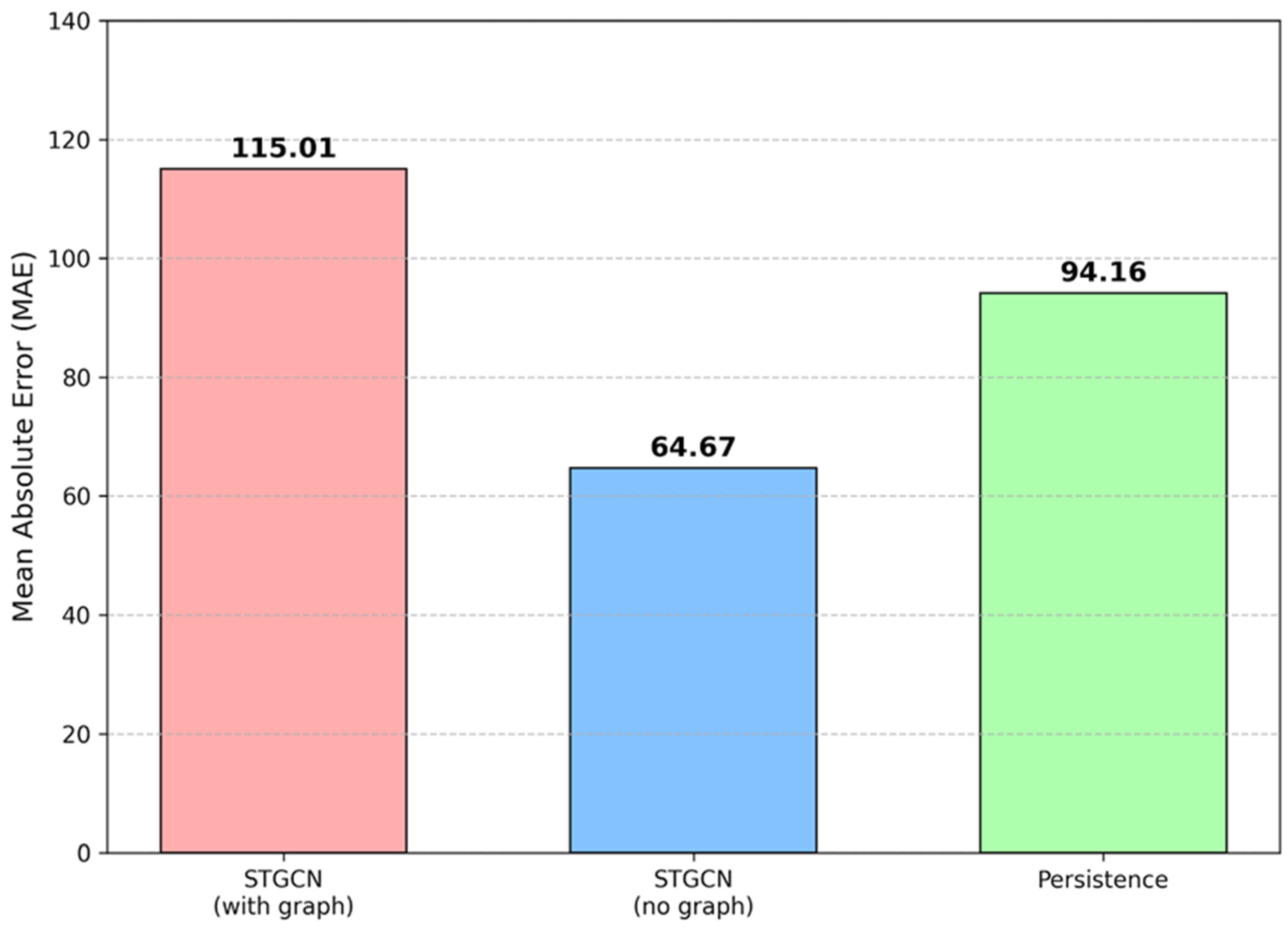
Table 4 presents the overall test performance on UrbanEV for the graph-usage ablation. Averaged over S = 5 seeds (0–4), the no-graph variant achieves a superior MAE of 66.53 ± 1.71, outperforming both the with-graph STGCN (MAE 116.21 ± 5.43) and persistence (MAE 94.16). Additional comparisons with alternative predefined static priors (distance-based $A_{dist}$ and correlation-based $A_{corr}$) are reported in Table S3; although $A_{corr}$ reduces the error relative to $A_{data}$, both remain substantially worse than the no-graph ablation. Corresponding improvements are observed across RMSE (283.22 ± 7.99 vs. 393.74 ± 32.78 with-graph), NMAE, and other metrics, indicating that the static graph introduces detrimental effects. This advantage is statistically reliable under paired tests on node-wise MAE across forecasting horizons (two-sided Wilcoxon signed-rank test with Benjamini–Hochberg adjustment; see Table S1). This suggests a mismatch between the predefined graph and true dependencies, where spatial aggregation propagates irrelevant signals or dilutes node-specific patterns. Practically, this warns against assuming graphs are always beneficial; empirical validation is essential, and simpler temporal models may suffice or excel in mismatched scenarios. The same comparison is visualized in Figure 3.

Graph diagnostics: evidence of graph–data mismatch. To substantiate whether a predefined static graph aligns with the forecasting dependency structure, we report two complementary diagnostics computed on the training split. First, dependency lift Δcorr measures whether edges preferentially connect more dependent node pairs than non-edges by comparing the average absolute Pearson correlation |$corr\left(y_i, y_j\right)$| over edge pairs versus randomly sampled non-edge pairs. Second, the Dirichlet energy $E_D= Tr\left(Y^{T}L Y\right)$ (with graph Laplacian L) quantifies how strongly the target signal varies across connected nodes; a larger $E_D$ indicates that the graph links nodes with dissimilar targets, making spatial smoothing potentially harmful. On UrbanEV, we observe negative (or near-zero) dependency lift together with markedly higher Dirichlet energy for the predefined adjacency, supporting the hypothesis that the static prior mixes weakly related or heterophilic node signals. For interpretability, we additionally visualize the distribution of |corr| for edge versus non-edge pairs, which shows substantial overlap and limited separation, consistent with mismatch.

5.2. UrbanEV: Horizon-Wise Error Growth

Table 5. UrbanEV horizon-wise MAE (H = 6): graph-usage ablation (representative run, seed = 0). Notes: Multi-seed overall metrics are reported in Table 4.

Model	h = 1	h = 2	h = 3	h = 4	h = 5	h = 6
STGCN (with graph)	109.7443	109.0027	113.2403	114.8425	117.5648	125.6499
STGCN (no graph; A = I)	46.1499	56.7784	64.1138	69.4089	73.354	78.1961
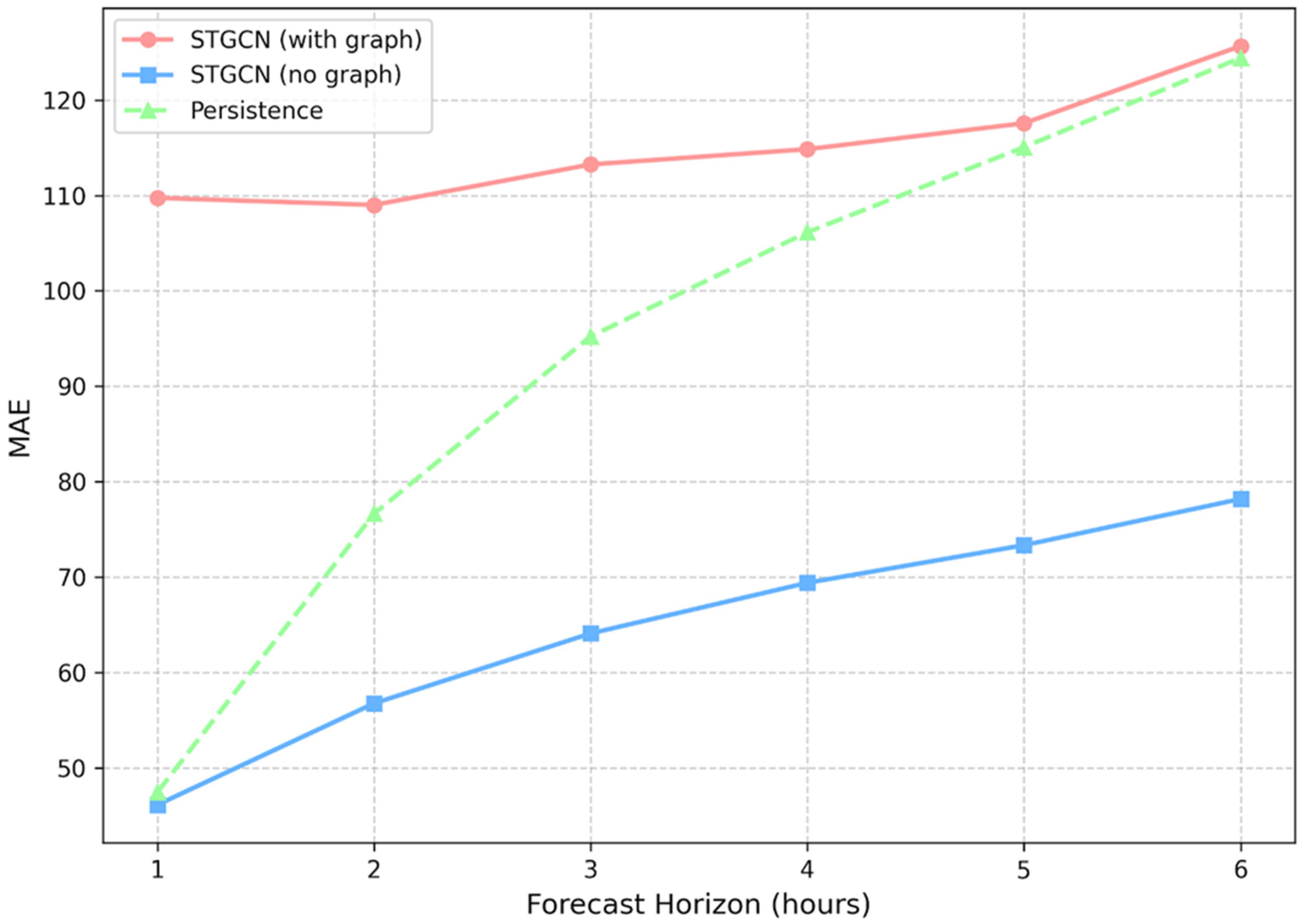
Persistence	47.4658	76.6416	95.2259	106.1394	115.0556	124.409

details the MAE across individual horizons (h = 1 to 6) on UrbanEV for a representative run (seed = 0). The errors escalate with the horizon for all models, reflecting increasing uncertainty in longer-term predictions. Notably, the no-graph model starts with low error (46.15 at h = 1) and grows more gradually than with-graph (109.74 at h = 1, rising to 125.65 at h = 6), consistent with the multi-seed aggregate gaps reported in Table 4.

Compared to persistence, no-graph is competitive at short horizons and superior at longer ones, highlighting the value of learned temporal dynamics even without spatial components. The horizon-wise error growth is plotted in Figure 4.

5.3. UrbanEV: Feature Ablation

Table 6. UrbanEV feature ablation results (test set). Notes: Lower is better. The backbone architecture is fixed; only input channels differ.

Feature Set	MAE	RMSE	NMAE	NRMSE	WAPE	MaskedMAPE
vol_only	100.4312	459.537	0.4285	1.9607	0.4285	0.5622
vol_dur	94.8619	440.7527	0.4047	1.8805	0.4047	0.4816
vol_dur_occ	90.2871	430.9474	0.3852	1.8387	0.3852	0.4945
vol_dur_occ_price	91.6367	431.5474	0.391	1.8413	0.391	0.5179
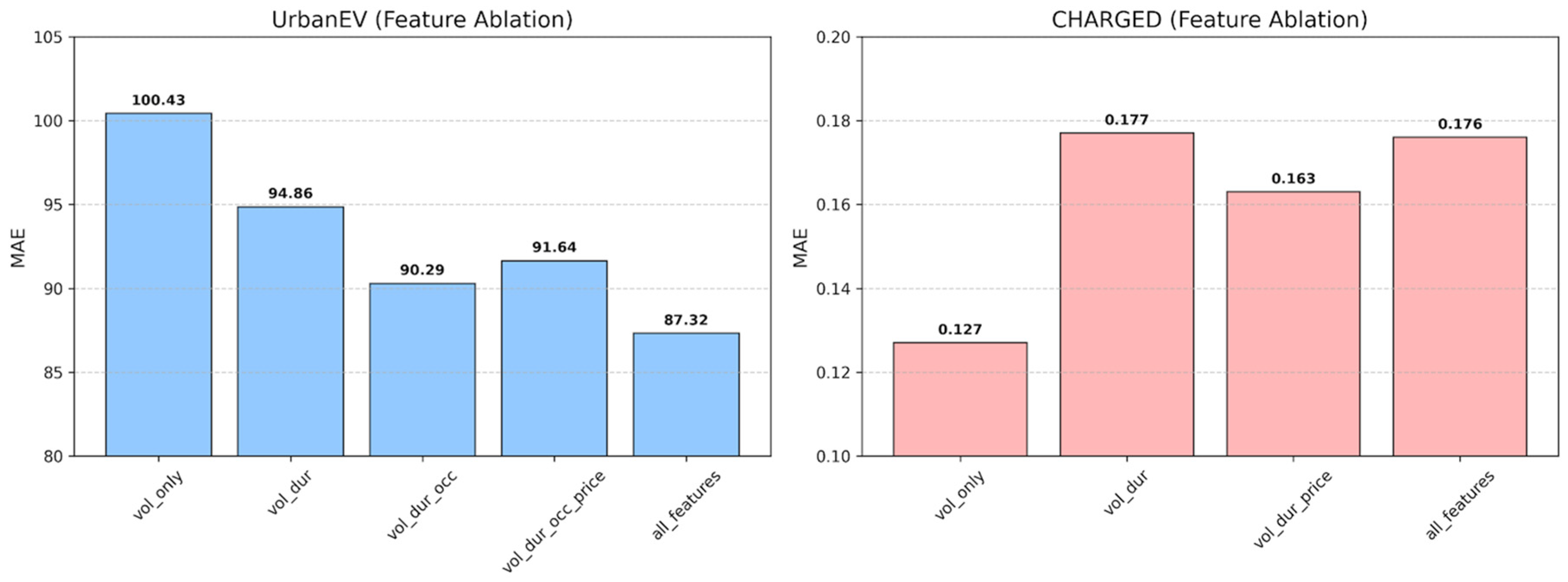
all_features	87.3196	421.7973	0.3726	1.7997	0.3726	0.5182

summarizes the feature ablation results on UrbanEV’s test set. Starting with vol_only (MAE 100.43), adding the duration (vol_dur: MAE 94.86) and occupancy (vol_dur_occ: MAE 90.29) yields progressive improvements, with all_features achieving the lowest MAE (87.32). This pattern holds across metrics, suggesting that occupancy and price signals offer complementary cues for refining predictions beyond volume autoregression.

For instance, occupancy may indicate impending capacity constraints, while prices influence user decisions, enhancing the model’s ability to anticipate shifts.

5.4. CHARGED: Feature Ablation and Strong Short-Term Autocorrelation

Table 7. CHARGED feature ablation results (test set). Notes: MaskedMAPE is computed over entries with |y| > 1.0. Persistence metrics are included for reference under the same masking rule.

Feature Set	MAE	RMSE	NMAE	NRMSE	WAPE	MaskedMAPE
vol_only	0.1273	0.7068	0.0039	0.0214	0.0039	0.0126
vol_dur	0.1766	0.7866	0.0053	0.0238	0.0053	0.017
vol_dur_price	0.163	0.775	0.0049	0.0235	0.0049	0.016
all_features	0.1756	0.7348	0.0053	0.0222	0.0053	0.0181
Persistence (reference)	0.1393	0.7979	0.0042	0.0241	0.0042	0.004

reports the feature ablation on CHARGED. Unlike UrbanEV, the simplest input (vol_only) achieves the best MAE, slightly outperforming persistence and consistently outperforming richer feature sets. This pattern suggests that CHARGED charging volumes are strongly predictable from short-term autocorrelation, while additional covariates (e.g., duration or prices) may introduce weakly informative or noisy signals under a static modeling assumption. To make this interpretation concrete, we further analyze feature–target associations using correlation and mutual-information diagnostics in Section 5.5. A cross-dataset summary of feature ablations is provided in Figure 5.

5.5. Feature-Target Association Diagnostics

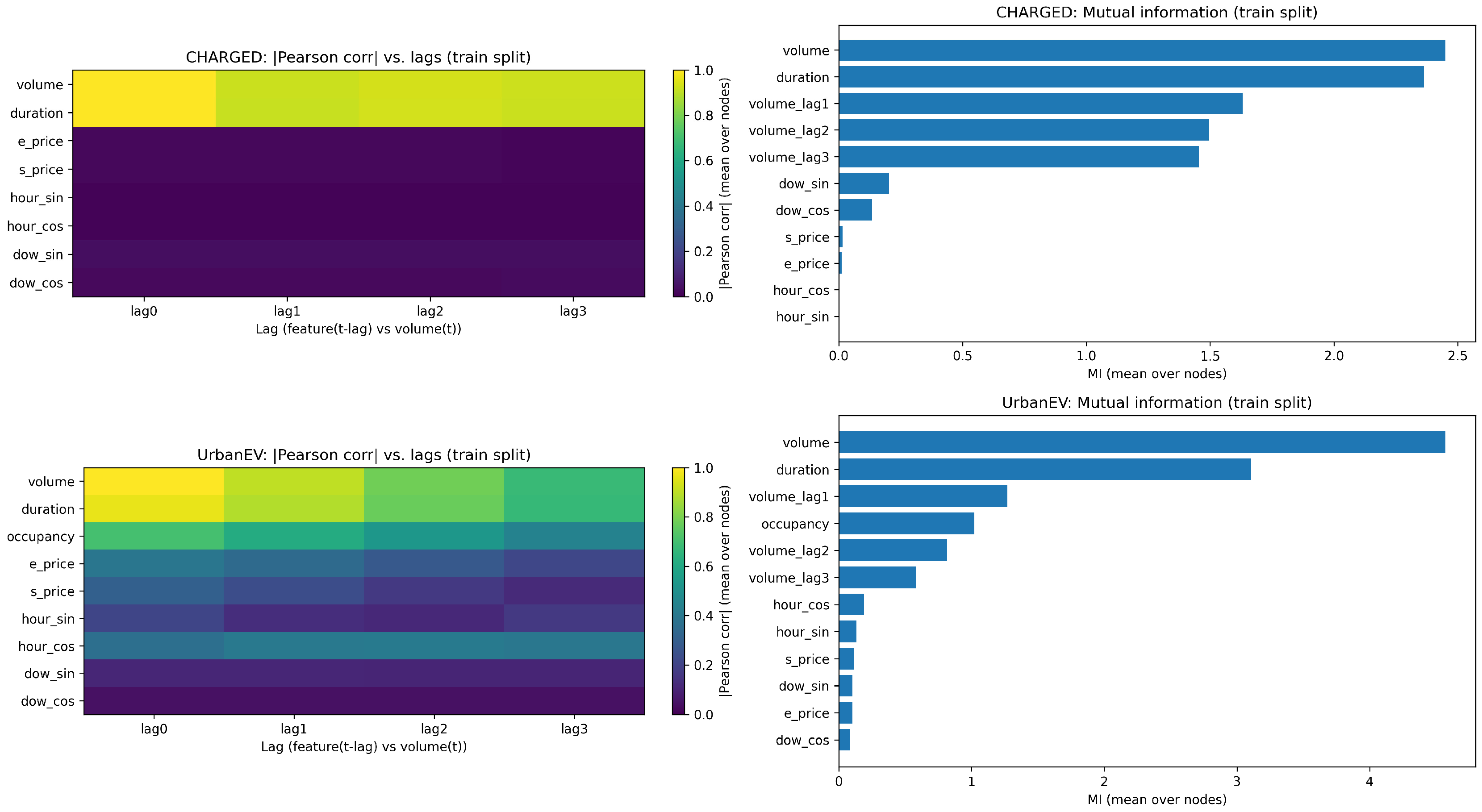
To explain why adding covariates can degrade the performance on CHARGED, we quantify how strongly each feature is associated with the target volume. We compute (i) the Pearson correlation between each candidate feature and the target volume (both contemporaneous and with short lags) and (ii) mutual information (MI) as a nonlinear dependency measure. Figure 6 summarizes these association diagnostics. In CHARGED, several covariates exhibit weak and unstable associations with the target compared to the strong self-dependency of volume, which is consistent with the superior performance of vol_only. In contrast, UrbanEV shows more consistent associations between the volume and selected covariates (e.g., occupancy/prices), matching the observed benefits of richer feature sets.

We compute the Pearson correlations not only contemporaneously but also with 1–6 h lags of candidate covariates (and of the target), and we observe that the covariate–target associations remain weak on CHARGED.

These diagnostics support a practical interpretation: when exogenous signals are weakly coupled to the short-horizon target or are affected by noise, missingness, or non-stationary policies, concatenating them as static inputs can increase the effective learning burden and harm generalization. This motivates either (i) feature selection guided by dependency diagnostics or (ii) adaptive mechanisms (e.g., attention or regime-aware conditioning) to integrate covariates only when they are predictive.

5.6. Summary of Key Findings

Across both datasets, our ablations reveal the following: (i) static graphs require validation, as mismatches can harm performance (e.g., UrbanEV degradation), and (ii) feature benefits such as context-specific-richer sets aid UrbanEV but may hinder CHARGED due to noise. These motivate adaptive approaches and multi-task learning for robust cross-node and exogenous integration.

6. Discussion

6.1. Why Might Static Graphs Hurt?

Static graphs derived from geography or administratively defined topology encode a convenient spatial prior, but they do not guarantee alignment with the dependency structure of the forecasting target. From the perspective of heterophily, a graph can be “structurally plausible”, yet still connect nodes whose target signals are weakly related or even anti-correlated due to competition, functional substitutability, or policy-driven rerouting. In such cases, neighborhood aggregation in graph convolutions effectively mixes dissimilar signals, increasing the bias and degrading multi-step forecasts. This mechanism is consistent with our mismatch diagnostics: on UrbanEV, the predefined adjacency yields a negative dependency lift (Δcorr = −0.0436) together with a much larger Dirichlet energy ($E_D$ = 4.43 × 10⁵; Table S2), indicating that graph edges do not preferentially connect more dependent node pairs and that spatial smoothing tends to mix dissimilar target signals. In contrast, CHARGED shows near-zero dependency lift (Δcorr ≈ 0.0009) and much lower Dirichlet energy ($E_D$ = 8.31 × 10²; Table S2), suggesting that the distance-based kNN prior is not strongly mismatched in correlation structure, and that the performance degradation there is more plausibly attributed to weak covariate–target coupling rather than topology alone.

Moreover, city systems are temporally non-stationary. Even if a static graph matches dependencies on average, the strength and sign of cross-node relations can vary across regimes (e.g., pricing changes, capacity constraints, events, or seasonal effects), making a fixed topology an unreliable inductive bias for all horizons and periods. Under such regime shifts, exogenous features or local temporal patterns may be more predictive than spatial mixing, which helps explain why the no-graph variant can outperform on some settings. These observations motivate two practical directions: (i) incorporate lightweight diagnostics (e.g., Δcorr and $E_D$) to validate whether a predefined graph is aligned with the target before relying on message passing and (ii) adopt adaptive or gated mechanisms (e.g., dynamic graphs or attention-based conditioning) that can selectively enable spatial interactions when they are empirically supported.

6.2. Limitations and Future Work

First, regarding model baselines, our study focuses on isolating the specific contribution of the graph module within a unified STGCN framework. While we compared against a persistence baseline, we acknowledge that additional deep temporal baselines (e.g., LSTM, GRU, or Transformer-based models) could offer further context. However, it is important to note that our No-Graph STGCN variant ($\mathrm{A}=\mathrm{I}$) removes cross-node message passing while preserving the same temporal convolutional backbone, residual design, and model capacity and is thus functionally equivalent to an equal-capacity per-node Temporal Convolutional Network (TCN) under the same training protocol. This makes the no-graph ablation a strong controlled temporal baseline for attributing performance differences to the spatial prior.

Second, regarding experimental robustness, we now report multi-seed results (mean ± std over S = 5 seeds) for the main UrbanEV graph-usage ablation (Table 4), complemented by paired significance tests on node-wise errors (Table S1). Some secondary ablations remain single-seed due to compute constraints; for those settings, we report point estimates and frame conclusions cautiously, prioritizing effects that are large relative to typical variability.

Third, regarding graph construction, our study uses predefined static graphs (e.g., distance-based or dataset-provided adjacency). Future work will expand comparisons to adaptive and dynamic graph learning architectures (e.g., Graph WaveNet, AGCRN) to test whether learned or time-varying dependencies can better match the forecasting target and recover performance beyond static priors.

6.3. Implications for Practice

Practitioners should adopt a validation-driven approach; begin with strong temporal baselines (persistence, no-graph), incorporate graphs only upon demonstrated gains, and select features using hypothesis-tested out-of-sample evidence. This minimizes deployment risks in smart-city settings, where mismatched inductive biases can translate into suboptimal operational decisions.

7. Conclusions

We presented an empirical study of graph and feature ablations for city-scale EV charging demand and road-network flow forecasting under a unified STGCN-based pipeline. Across two datasets with different scales, we found that simple static graph priors can reduce accuracy when they are mismatched with the underlying dependency structure of the forecasting target, while exogenous features provide dataset-dependent benefits. Our results emphasize the importance of controlled ablations and strong temporal baselines when deploying spatio-temporal models in practice. Future work will expand comparisons to additional state-of-the-art baselines, adaptive/dynamic graph learning, and broader multi-task settings linking mobility and energy systems.

Importantly, our results do not imply that static graphs are universally harmful. Rather, they show that a convenient static prior (e.g., proximity- or administrative-based adjacency) can reduce accuracy when it does not match the true dependency structure of the forecasting target. When the prior is informative (e.g., topology-consistent or correlation-aligned) or when the graph is learned/adaptive with proper regularization, spatial modeling may still yield gains. Hence, we recommend validating graph utility via no-graph ablations and lightweight diagnostics before committing to graph-based deployments.