Road Slippery State-Aware Adaptive Collision Warning Method for IVs

Abstract

To address critical limitations in conventional forward collision warning (FCW) systems including inadequate road condition detection accuracy, significant warning area prediction errors, and poor environmental adaptability on wet/snow-covered roads, this study develops an adaptive collision warning framework based on real-time road slippery states recognition. An enhanced ED-ResNet50 model is proposed, incorporating grouped convolutions within the backbone network and embedding ECA attention mechanisms after the second/third residual blocks alongside DDS-DA modules after the fourth block, significantly improving discriminative capability for pavement texture analysis under adverse conditions. This vision-based recognition system synchronizes with YOLOv8 for preceding vehicle detection, enabling the construction of a friction-sensitive safety distance and the time-to-collision model that dynamically calibrates warning thresholds according to instantaneous vehicle velocity and road adhesion coefficients. Real-vehicle validation demonstrates an 8.76% improvement in overall warning accuracy and 7.29% reduction in lateral and early false alarm rates compared to static-threshold systems, confirming practical efficacy for safety assurance in inclement weather.

1. Introduction

Forward Collision Warning (FCW) systems constitute a critical safety component in intelligent vehicles, significantly reducing frontal collision incidents. However, their effectiveness substantially diminishes under adverse road conditions such as wet or snowy surfaces, where reduced tire–road friction coefficients extend braking distances and elevate collision risks, potentially leading to severe casualties and property damage [1]. While machine vision-based FCW solutions offer cost efficiency and environmental perception advantages over LiDAR or millimeter-wave radar approaches [2,3,4], existing systems exhibit two fundamental limitations: insufficient robustness in road states recognition against environmental interference, and inflexible warning thresholds that are unadapted to dynamic friction variations.

Current research predominantly employs deep learning for road condition classification. The method based on deep learning mainly extracts the image feature information through the neural network [5]. Gin et al. [6] pioneered a lightweight RefNet architecture utilizing specialized Ref-Block residual units, optimized via TensorRT acceleration. Chen et al. [7] implemented adversarial neural networks to eliminate road surface shadows prior to residual network-based classification. Yang et al. [8] developed an adaptive illumination correction algorithm using two-dimensional gamma functions, subsequently applying ResNet18 for pavement analysis. Despite these advancements, prevailing methods remain vulnerable to environmental artifacts such as reflections and shadows, constraining feature discriminability and cross-scenario generalization. In view of the above problems, this paper proposes a recognition method of slippery road surface based on an improved ResNet50 network, in order to improve the recognition accuracy of the bad road surface.

The integration of real-time road condition assessment into forward collision warning (FCW) frameworks represents an emerging research focus within intelligent vehicle systems [9,10,11]. Existing methodologies, however, exhibit critical constraints across operational scenarios: Cai Chuangxin et al. [12] established a lane detection-dependent safety distance model that remains inapplicable in unstructured environments lacking clear road markings. He Yong et al. [13] devised a vehicle cut-in identification method combining lane occupancy thresholds with turn signal verification, yet this approach demonstrates severe performance degradation under low-visibility conditions such as rain or snow due to inherent sensor sensitivity limitations. Hiraoka et al. [14] introduced a collision probability metric predicated on constant velocity assumptions, fundamentally misaligned with real-world variable-speed traffic dynamics. Shen Haiyang et al. [15] developed speed-tiered safety zoning without incorporating tire–road friction coefficients, neglecting their decisive impact on braking kinematics across diverse pavement conditions. Zhu Bing et al. [16] proposed an adaptive longitudinal collision warning strategy based on the estimation of road adhesion coefficient. However, the estimation of road adhesion coefficient is based on a dynamic model rather than on-board vision, so the model method has the problem of time lag, and it can only obtain high estimation accuracy when the tire is in a large slip range. Collectively, environmental interference undermines feature extraction robustness during target and road states identification; in addition, fixed warning thresholds fail to accommodate friction-induced braking variance, elevating false alarm rates and critically compromising FCW efficacy under adverse road conditions.

In view of the problems existing above, this paper presents an intelligent vehicle adaptive collision warning method based on the road slippery states recognition. The main idea is that an enhanced ED-ResNet50 model is proposed, significantly improving discriminative capability for pavement texture analysis under adverse conditions. Furthermore, this vision-based recognition system synchronizes with YOLOv8 for preceding vehicle detection, enabling the construction of a friction-sensitive safety distance and the time-to-collision model that dynamically calibrates warning thresholds; timely warning is provided for possible collision situations. The main innovations of this paper are as follows:

(1)

An augmented road recognition model (ED-ResNet50) is constructed to enhance feature extraction through integrated grouping convolutions and hybrid attention mechanisms, which strengthens the discriminative capability for wet/snowy pavement textures while suppressing interference from shadows and reflections, improving recognition robustness in complex environments.

(2)

An adaptive collision warning strategy is proposed to synthesize YOLOv8-based vehicle detection with friction-sensitive kinematics, which dynamically recalibrates safety thresholds by correlating instantaneous vehicle velocity with road adhesion coefficients, overcoming the rigidity of conventional fixed-threshold approaches.

(3)

An embedded validation framework is deployed to execute continuous road-state classification, target detection, and adaptive warning generation on real-vehicle platforms, which confirms operational stability and practical applicability across diverse dry, wet, and snowy scenarios within intelligent driving systems.

2. The Recognition of Road Slippery States

2.1. System Architecture

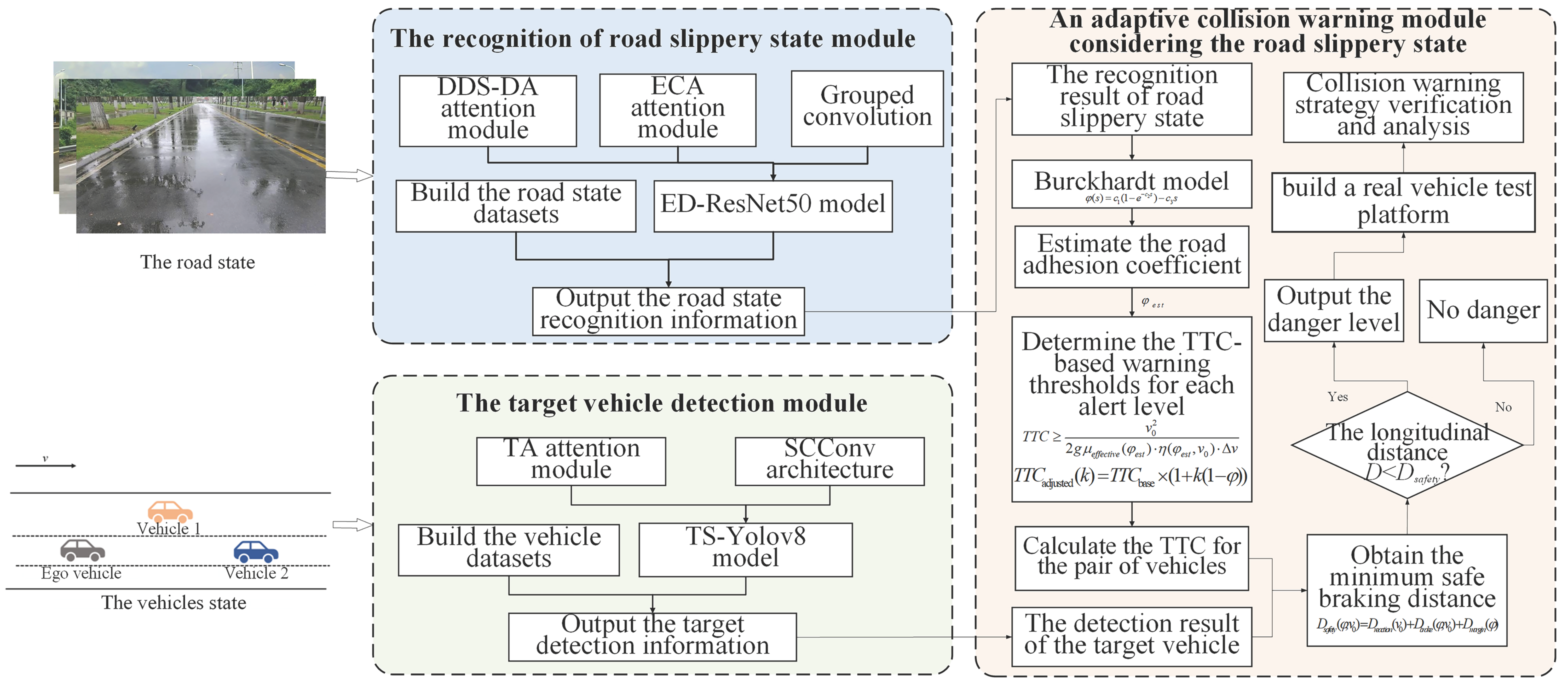
This study develops the road slippery states-aware adaptive collision warning method for IVs, as shown in Figure 1. The system follows a closed-loop workflow integrating perception, decision-making, and warning. An enhanced ED-ResNet50 network classifies the road surface (e.g., dry, wet, or snowy) from monocular camera images, and the result is mapped to a physical road adhesion coefficient ($\phi$) via a Burckhardt model lookup. This $\phi$ value, together with the host vehicle speed and relative kinematics from a YOLOv8-based detector, feeds into a friction-sensitive safety distance model and a time-to-collision (TTC) calculation. Crucially, the warning thresholds are dynamically adjusted based on real-time $\phi$ and speed, enabling earlier warnings on low-friction roads to compensate for longer braking distances.

This collision warning system is mainly composed of three parts: (1) the recognition of road slippery states module, shown in Section 2.2; (2) the target vehicle detection module, see Section 3.1 for details; and (3) an adaptive collision warning module considering the road slippery states, shown in Section 3.2 and Section 3.3; this section detailed the method of road slippery state recognition.

2.2. ED-ResNet50 Model

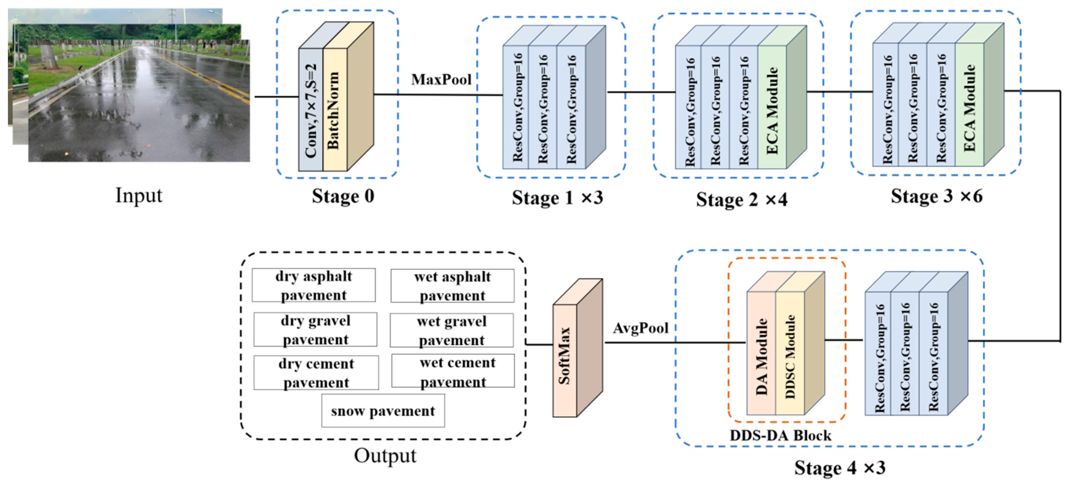
This study categorizes the road surfaces into seven distinct types: dry asphalt, dry cement, dry gravel, wet asphalt, wet cement, wet gravel, and snow-covered pavement. To achieve accurate and efficient identification of road slippery states, this paper conducts adaptive optimization based on the ResNet50 model, such as adjusting the structure of the ResNet50 backbone network and introducing the attention mechanism, in order to build a more efficient recognition model [17,18,19]. ED-ResNet50 is shown in Figure 2, and its key modifications include:

(1)

In order to improve the model’s ability to capture features of different scales, the ED-ResNet50 model introduces an ECA attention mechanism module at the end of the second and third residual modules according to the functions of each residual module of the residual network model, so as to enhance the model’s ability to extract middle-level features.

(2)

In the fourth residual module, a DDS-DA attention module consisting of Dilated Depthwise Separable Convolution and a Dual Attention Module is introduced, which can improve the model’s ability to extract high-level features and strengthen the expression ability of features and the positional correlation between features by combining local and global feature information.

(3)

The ordinary convolution in the main model is replaced with group convolution, which can reduce the number of parameters in the model, making it lightweight and improving the detection speed of the model.

2.2.1. ECA Attention Module

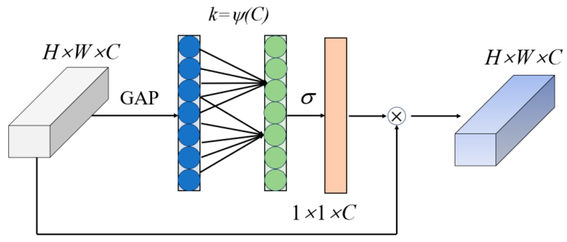
Within the ResNet50 architecture, the first residual module is mainly responsible for processing the original feature map of the network input, which is not suitable for adding the attention mechanism. The second and third residual modules are responsible for extracting medium and low-level features, so the ED-ResNet50 model introduces an ECA attention module at the end of the second and third residual modules. The ECA module can enhance channel and spatial information, improve feature representation, and thus improve the overall performance of the network [20,21]. The structure of the ECA attention mechanism is shown in Figure 3. The model feeds the input feature map with scale $H\times W\times C$ into the global average pooling layer (GAP).

$$z_c={\displaystyle \frac{1}{H\times W}}{\displaystyle \sum _{i=1}^H{\displaystyle \sum _{j=1}^W{X}_{i,j,c}}}, z\in R^C$$

(1)

After global average pooling, the feature map becomes a feature vector z with scale $1\times 1\times C$. Then, the feature vector z undergoes a 1D adaptive convolution with a kernel size k. After the convolution operation, the output is a feature vector s with length C. The vector s is then activated by the Sigmoid function to obtain the attention weight α, where each element corresponds to the weight of each channel in the input feature map. The weighted feature map is obtained by multiplying the attention weight α with each channel of the input feature map. The size of the weighted feature map is still $H\times W\times C$. The calculating formula for the size k of the one-dimensional adaptive convolution kernel is as follows:

$$k=\psi (C)=\left|{\displaystyle \frac{{\log }_2(C)}{\gamma }}+{\displaystyle \frac{b}{\gamma }}\right|$$

(2)

where γ is usually deemed as 2 and b is deemed as 1.

2.2.2. DDS-DA Attention Module

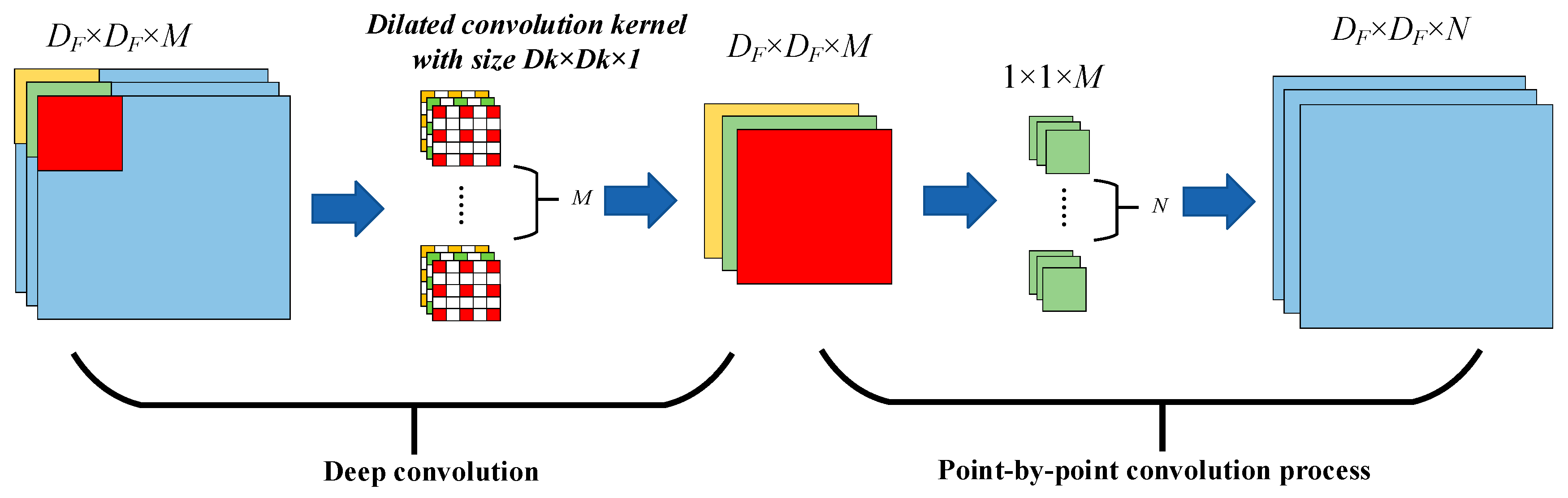
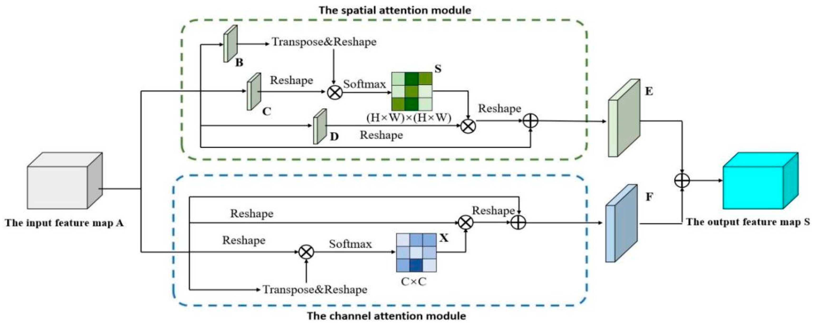
The fourth residual module in the ResNet50 structure is mainly responsible for extracting advanced features, and the DDS-DA attention module is introduced at the end of the fourth residual module. The DDS-DA attention module is composed of the Dilated Depthwise Separable Convolution and the Dual Attention Module. The DDS-DA attention module can improve the model’s ability to extract high-level features, and it can capture global dependencies and local details, thus improving the overall performance and robustness of the model [22].

The process of Dilated Depthwise Separable Convolution is shown in Figure 4. It can be seen that the hollow depth separable convolution can reduce the calculation amount of the model, expand the receptive field of the model, and increase the computational efficiency of the model while ensuring that the output has the same feature map as the ordinary convolution.

The Dual Attention Module mainly includes two sub-modules: the Channel Attention Module and Position Attention Module. The structure of the Dual Attention Module is shown in Figure 5.

To fully utilize the long-range context information, the outputs of the two attention modules are transformed through the convolutional layer, and the element-wise summation is performed to achieve feature fusion. Finally, the convolutional layer generates the final prediction map S.

2.2.3. Grouped Convolution

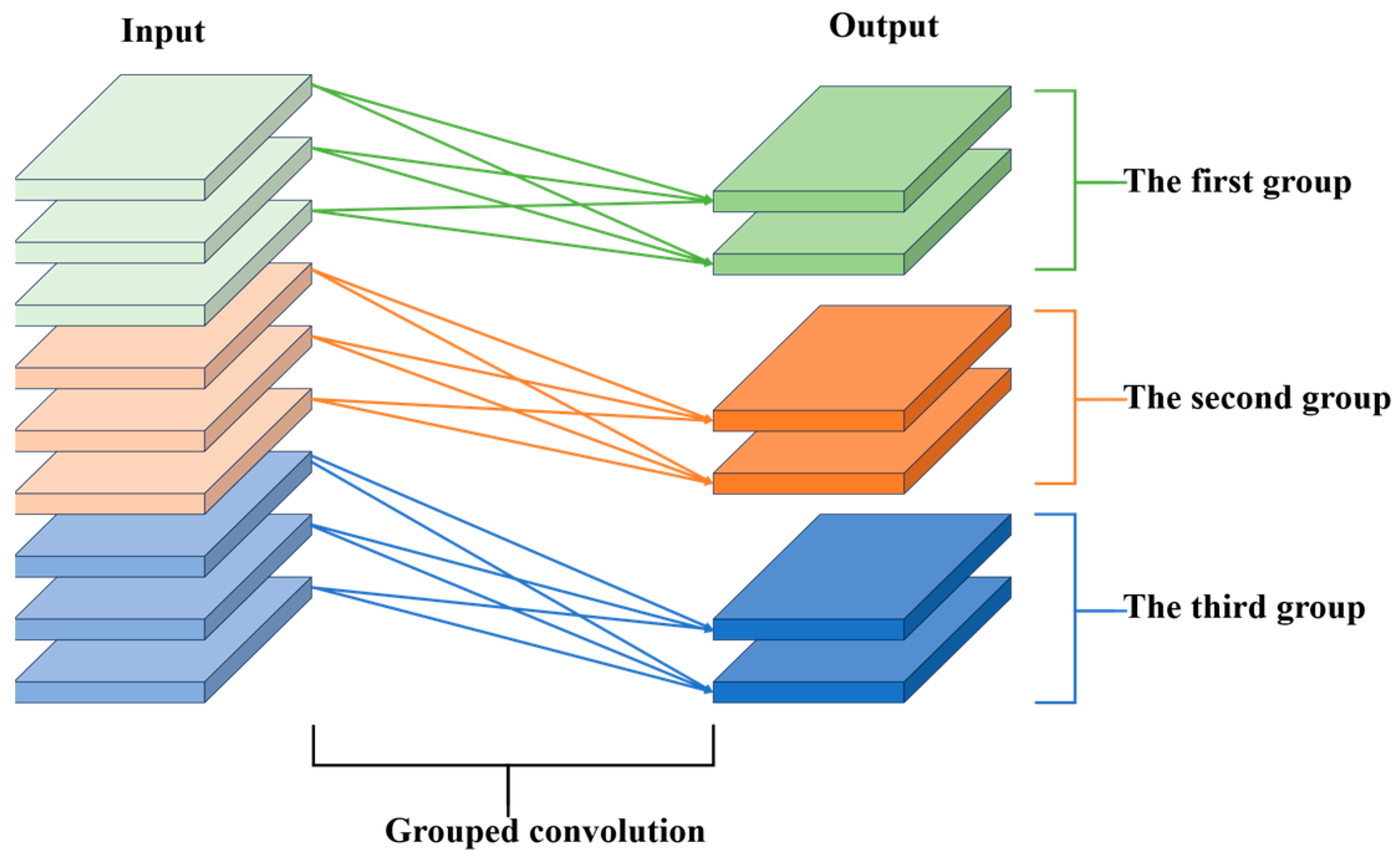
The concept of grouped convolution originated from the AlexNet model, which is a convolution operation used for processing input feature maps. Grouped convolution divides the input channels into multiple groups, and each group is assigned an independent set of convolution kernels. Each group performs convolution independently, and calculation efficiency is improved through parallel processing. The operation of grouped convolution is shown in Figure 6.

Group convolution divides the feature map of size $H\times W\times C$ into m groups along the channel dimension, denoted as $X\in \left[x_0,x_1,\dots x_{m-1}\right],x_i\in {ℝ}^{H\times W\times (C/m)}$, and performs independent convolution operation on each x_i. The calculation formula for the number of parameters and the floating-point operations of each layer is as follows:

$$params={\displaystyle \frac{C_i\times C_0\times k^2}{m}}$$

(3)

$$FLOPs={\displaystyle \frac{C_i\times C_0\times k^2\times H\times W}{m}}$$

(4)

where C_i represents the number of input channels for the feature map, C₀ represents the number of output channels for the feature map, k is the size of the convolution kernel, usually there is $C_i=C_0$.

Grouped convolution can effectively reduce the number of parameters and computations of the model, making it more lightweight. Additionally, grouped convolution allows the model to learn different feature representations across different groups, helping the model to extract richer and more diversified features.

2.3. Visual-Based Estimation of the Road Adhesion Coefficient

A hybrid, physics-informed strategy is adopted to estimate the road-tire adhesion coefficient. This approach combines robust visual classification with a well-established tire–road friction model (The Burckhardt model) to ensure physically plausible and reliable estimates.

The Burckhardt model is an estimation model for the road adhesion coefficient derived from a large number of experiments, which represents the relationship curve between the adhesion coefficient and slip rate under various road conditions, and is widely used in vehicle dynamics [23]. The Burckhardt model describes the relationship between the road adhesion coefficient and slip rate through the following equation:

$${\phi }_{est}(s)=(c_1(1-e^{-c_{2}s})-c_{3}s)$$

(5)

where ${\phi }_{est}$ is the visual-based estimation of the adhesion coefficient, $c_1,c_2$ and $c_3$ are three fitting parameters, the specific values of which are determined by the current states of the road, and s is the slip ratio.

Based on the resultant recognition of road slippery states in Section 2.2, the core of our work lies in establishing a reliable mapping from visual semantics to physical parameters. The logic is as follows: (1) Input: Road surface categories output by ED-ResNet50 (e.g., “wet asphalt”). (2) Mapping: This category corresponds to established knowledge in vehicle engineering. (3) Output: Retrieve the recognized and representative Burckhardt parameters under this category from the knowledge base (i.e.,

Table 1. The Burckhardt model parameters under different road surfaces.

Type of Pavement	c1	c2	c3
dry asphalt pavement	1.28	23.99	0.52
dry cement pavement	1.20	25.17	0.54
dry gravel pavement	0.85	12.50	0.30
wet asphalt pavement	0.70	33.82	0.35
wet cement pavement	0.65	24.59	0.25
wet gravel pavement	0.85	15.00	0.20
snow pavement	0.20	94.13	0.06

). The values of $c_1,c_2$ and $c_3$ for each road surface are shown in Table 1.

3. Vehicle Collision Warning Strategy

The YOLOv8 is used to detect the lead vehicle, and the current road surface condition is determined by Section 3.2 mentioned above. The Burckhardt model is used to estimate the adhesion coefficient of different road surface conditions. Then synchronized YOLOv8-based vehicle detection enables dynamic calibration of safety distances and the time-to-collision through a friction-sensitive kinematic model that continuously adjusts warning thresholds according to instantaneous velocity and quantified road slipperiness.

3.1. Vehicle Detection

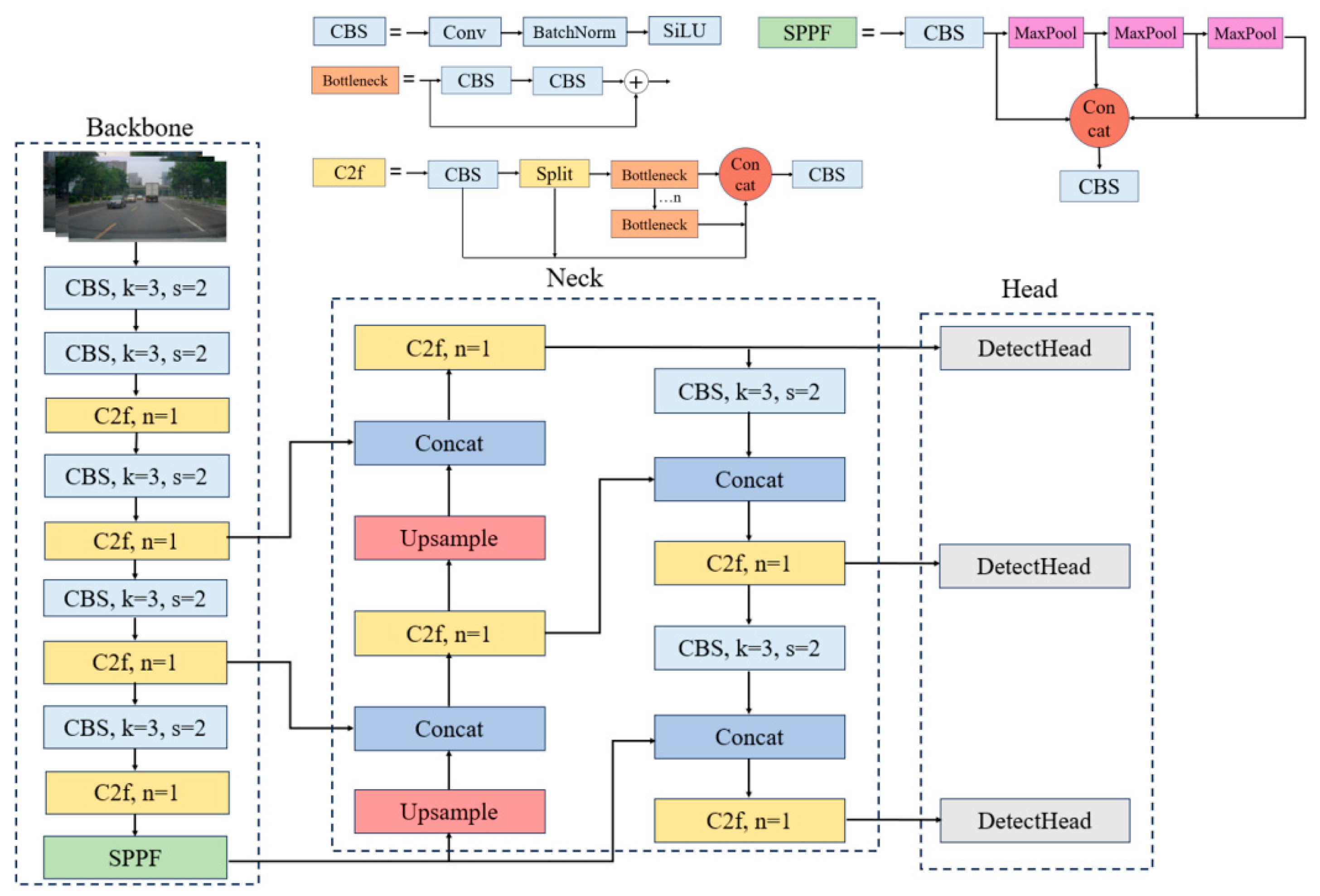
Because Fast-RCNN [24] and Faster-RCNN [25] have relatively low detection performance, a large number of parameters and a long processing time, they are not suitable for real-time detection tasks of dynamic targets in traffic scenes. However, YOLOv5 and YOLOv8, as lightweight models, significantly improve recognition accuracy compared to Fast-RCNN and Faster-RCNN, with fewer model parameters and faster processing speeds [26,27]. Therefore, this paper uses YOLOv8 as the target vehicle detection model. The structure of the YOLOv8 model is shown in Figure 7.

The backbone of YOLOv8 consists of CBS, C2f and SPPF. Among them, CBS is the basic convolutional structure, which includes convolution, batch normalization and SiLu activation function. C2f refers to C3 and YOLOv7 ELAN, and adopts parallel multi-gradient flow to enhance gradient information, while maintaining a lightweight structure, and mitigating gradient vanishing through residual connections. SPPF employs three times 5 × 5 max-pooling operations to combine multi-scale features of 5 × 5, 9 × 9, and 13 × 13, and adjusts the number of channels through convolution to match the input. Neck follows the YOLOv5 structure by replacing C3 with C2f, and directly inputs the feature maps from different stages into upsampling to reduce computation and information loss. Head adopts three detector heads to detect small, medium, and large targets, and separates classification and regression features with decoupled detector heads, which improves the flexibility of detection and the efficiency of classification [28,29].

After the target coordinates are obtained using Yolov8, the distance is further estimated. A monocular ranging model based on the camera imaging principle is employed in this study to calculate the distance to the preceding vehicle according to the similar triangle theorem [30].

3.2. A Driving Safety Early Warning Model with Adaptive Traffic Environment Characteristics

Considering the influence of road slippery states on the safety distance and the time-to-collision, a driving safety early-warning model with environment-adaptive characteristics is established, thereby enabling adaptive fused collision warning under different road surface conditions.

(1)

Minimum safe braking distance considering road slippery states.

In this paper, we refer to the work of the literature [31,32] and use real-time estimation of road friction coefficient to adjust the safe distance between vehicles; the minimum safe braking distance is shown in Equation (6):

$$D_{safety}(\phi ,v_0)=D_{reaction}(v_0)+D_{brake}(\phi ,v_0)+D_{ margin}(\phi )$$

(6)

Among them, the distance formula for the driver response period is calculated by:

$$D_{reaction}(v_0)=v_0\cdot (t_{driver}+t_{system})$$

(7)

where $t_{driver}$ denotes the driver’s reaction time, and $t_{system}$ is the time required to initiate system braking.

Due to the change complexity of the road adhesion characteristics in the actual braking process, the vehicle braking distance is given by:

$$D_{brake}(\phi ,v_0)={\displaystyle \frac{v_0^2}{2g\cdot {\mu }_{effective}(\phi )\cdot \eta (\phi ,v_0)}}$$

(8)

In order to reflect the influence of different road conditions on braking performance more realistically, the equivalent friction coefficient function can be introduced:

$${\mu }_{effective}(\phi )={\phi }_{est}\cdot \left[1+\alpha \cdot \exp (-{\displaystyle \frac{{({\phi }_{est}-{\phi }_{no\min al})}^2}{2{\sigma }^2}})\right]$$

(9)

where ${\phi }_{camera}$ is the visual-based estimation of road adhesion coefficient, ${\phi }_{no\min al}$ is the reference adhesion coefficient, $\alpha$ is the adhesion coefficient compensation factor, and $\sigma$ is the road surface type distribution parameter.

In addition, we can approximately calculate the braking efficiency adjustment factor $\eta (\phi ,v_0)$ using the following empirical Equation (10):

$$\eta (\phi ,v_0)={\eta }_0\left[1-{\beta }_1{\displaystyle \frac{v_0}{v_{\max }}}\right]\cdot [1-{\beta }_2\cdot (1-{\phi }_{est})]$$

(10)

where ${\eta }_0$ is the base braking efficiency, ${\beta }_1$ is the speed efficiency decay coefficient, and ${\beta }_2$ is the adhesion efficiency decay coefficient.

Furthermore, the safety margin formula is shown as follows:

$$D_{ margin}(\phi )=d_{base}\cdot \left(1+\gamma \cdot {\displaystyle \frac{1-\phi }{\phi }}\right)$$

(11)

where $d_{base}$ is the base safety margin, typically ranging from 2 to 3 m, and $\gamma$ is the adjustment coefficient.

(2)

TTC warning threshold considering road slippery states.

According to the TTC model, the time-to-collision is determined only by the relative distance and relative velocity between two vehicles. To ensure that the vehicle can safely come to a complete stop before a collision occurs, the TTC must satisfy the following inequality:

$$TTC\ge TT{C}_{base}(\phi ,v_0,\Delta v)={\displaystyle \frac{D_{brake}(\phi ,v_0)}{\Delta v}}$$

(12)

Substituting the braking distance formula yields the following expression:

$$TTC\ge {\displaystyle \frac{v_0^2}{2g{\mu }_{effective}({\phi }_{est})\cdot \eta ({\phi }_{est},v_0)\cdot \Delta v}}$$

(13)

Therefore, considering road slippery states, the TTC warning thresholds are adaptively determined according to the adhesion coefficient. As the road adhesion coefficient decreases, a higher TTC warning threshold is required.

When the uncertainty of the estimated adhesion coefficient is high, the formulation for adjusting the multi-level TTC warning thresholds based on the road adhesion coefficient is given as follows:

$$TT{C}_{\mathrm{adjusted}}(k)=TT{C}_{\mathrm{base}}\cdot [(1+k\cdot (1-\phi )]$$

(14)

where k is the adjustment factor, representing the influence of the road adhesion coefficient on TTC, with a value range of (0, 1).

In this study, the root mean square error (RMSE) is used as the objective function to iteratively optimize the adjustment factor, as shown in Equation (15).

$$J(k)={\displaystyle \frac{1}{N}}{\displaystyle \sum _{i=1}^N[TT{C}_{base}^{(i)}}(1+k(1-{\varphi }^{(i)}))-TT{C}_{base}^{(i)}){]}^2$$

(15)

The model is solved using gradient descent (GD) $k^{(t+1)}=k^{(t)}-\alpha {\displaystyle \frac{\partial J}{\partial k}}{|}_{k=k^{(t)}}$, and the optimal coefficient k* is returned when the iteration times reach the upper limit or $\left|J(k^{(t+1)})-J(k^{(t)})\right|<\epsilon$.

Finally, the value of k is set to 0.35, and the threshold values of the adjusting TTC based on the road adhesion coefficient are obtained, as shown in

Table 2. The threshold values of the adjusting TTC considering the road adhesion coefficient.

Road Surface Condition	Collision Warning Levels
	Level-1 Warning	Level-2 Warning	Level-3 Warning	No Warning
Dry asphalt road	t ≤ 1.64 s	1.64 s < t ≤ 2.73 s	2.73 s < t ≤ 5.45 s	t > 5.45 s
Dry concrete road	t ≤ 1.69 s	1.69 s < t ≤ 2.81 s	2.81 s < t ≤ 5.62 s	t > 5.62 s
Dry gravel road	t ≤ 1.81 s	1.81 s < t ≤ 3.02 s	3.02 s < t ≤ 6.04 s	t > 6.04 s
Wet asphalt road	t ≤ 1.85 s	1.85 s < t ≤ 3.08 s	3.08 s < t ≤ 6.15 s	t > 6.15 s
Wet concrete road	t ≤ 1.89 s	1.89 s < t ≤ 3.14 s	3.14 s < t ≤ 6.28 s	t > 6.28 s
Wet gravel road	t ≤ 1.96 s	1.96 s < t ≤ 3.27 s	3.27 s < t ≤ 6.54 s	t > 6.54 s
Snow-covered road	t ≤ 2.09 s	2.09 s < t ≤ 3.54 s	3.54 s < t ≤ 7.08 s	t > 7.08 s

.

3.3. Multi-Level Warning Strategy Integrating TTC and the Minimum Safe Braking Distance

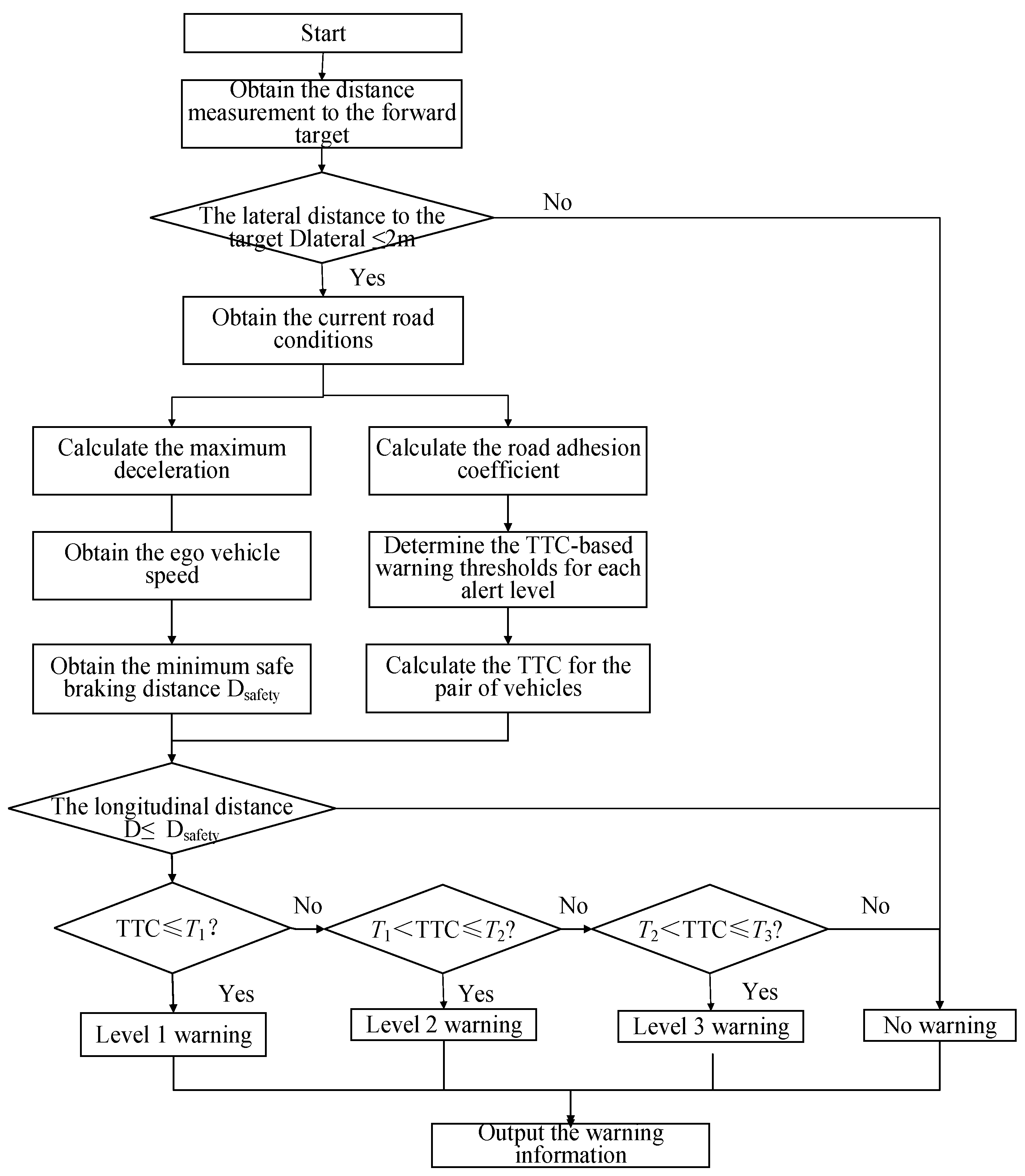
This paper considers the influence of the road adhesion coefficient on vehicle braking and improves the traditional TTC and the minimum safe braking distance models. Then, the improved TTC is combined with the minimum safe braking distance to combine dynamic and static information, thereby providing drivers with a more comprehensive risk assessment, enhancing the adaptability of the vehicle under different driving conditions, reducing the probability of false alarms and missed alarms, and increasing driver trust in the warning system. The process of the adaptive multi-level early warning strategy considering road surface conditions is shown in Figure 8. Firstly, the lateral distance obtained from monocular ranging is used for preliminary screening to exclude targets with excessively large lateral offsets. Subsequently, the model acquires the current road surface slippery state, calculates the road adhesion coefficient and maximum deceleration respectively, and then based on these parameters, the TTC thresholds at different levels and the minimum safe braking distance D_safety are determined. Based on the values of TTC and D_safety, the potential collision risk is classified into different warning levels:

When D ≤ D_safety and TTC ≤ T₁, the system classifies the situation as a level-1 warning, indicating an extremely dangerous state, and prompts the driver to take immediate braking action to avoid a collision.

When D ≤ D_safety, T₁ < TTC ≤ T₂, the system issues a level-2 warning, indicating a moderate risk and advising the driver to decelerate appropriately.

When D ≤ D_safety, T₂ < TTC ≤ T₃, a level-3 warning is triggered, indicating a low-level risk and reminding the driver to remain cautious.

When D > D_safety, the vehicle is considered to be in a safe state, and the system does not issue a warning. When D ≤ D_safety but TTC > T₃, although the distance between vehicles is smaller than the minimum safe braking distance, the relative speed is small or the speed of the preceding vehicle is higher than that of the ego vehicle; therefore, no imminent collision risk is assumed and no warning is issued.

4. Experimental Analysis and Result

4.1. Introduction of the Test Platform

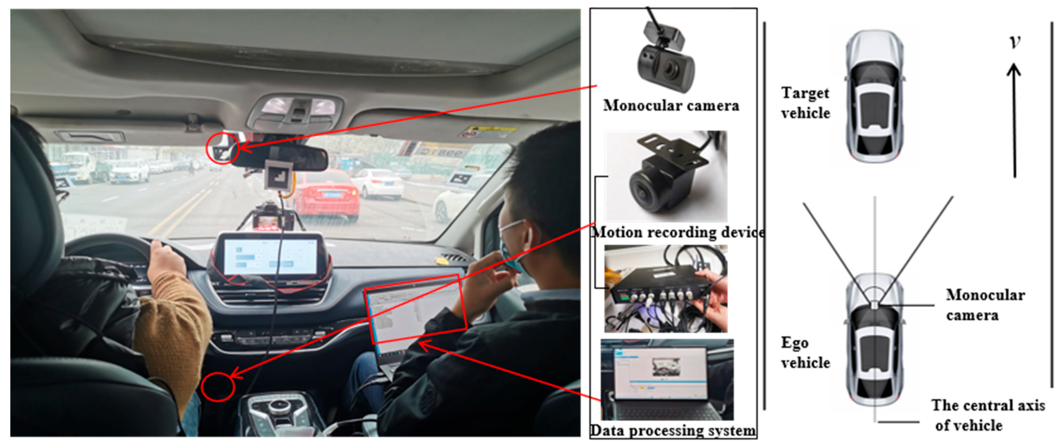
In this paper, a real-vehicle test platform equipped with a monocular camera is used to verify the effectiveness and real-time performance of the adaptive collision warning system based on road slippery states recognition. The platform architecture and warning scene are shown in Figure 9.

A real-vehicle test was conducted on a city road, using a single camera to capture video and perform detection. Meanwhile, the vehicle’s current speed and the driver’s braking time were recorded by the system. The pixel of the monocular camera is 1702 × 1276. The internal and external parameters of the camera obtained by Zhang Zhengyou calibration method [33] are shown in

Table 3. Camera calibration results.

Internal Parameter Type	Value
Equivalent focal length on the X axis (fx)	1316.6
Equivalent focal length on the Y axis (fy)	1330.7
The horizontal coordinate of the main point (u0)	869.6
The vertical coordinate of the main point (v0)	648.7
Radial distortion coefficient	(−0.3462, 0.1309)

.

4.2. The Result of Road Slippery States Recognition

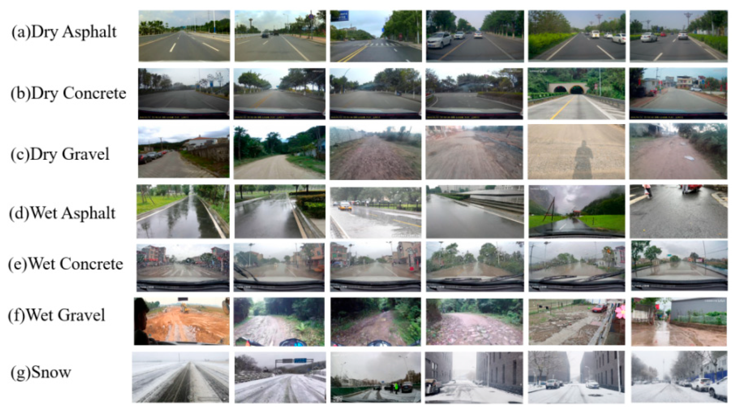
Image datasets are crucial for the recognition performance of neural networks. The dataset used in this paper primarily consists of the road states images captured on-site by on-board cameras and the images collected from publicly available datasets on the network (such as the RobotCar dataset, the KITTI dataset, the RTK dataset, etc.) [34,35,36]. Finally, the dataset is divided into seven categories, as shown in Figure 10. There are 1500 images for each category, and the dataset is divided into the training set, the validation set and the test set in the ratio of 8:1:1.

Then, the ED-ResNet50 model was used for recognition training. The specific parameter settings for the training in this study are shown in

Table 4. Training parameter setting.

Parameter Type	Value
Input size (pixels × pixels)	224 × 224
Initial learning rate	0.01
batch size	32
Number of categories	3
Number of training iterations	100

. The model is evaluated from two aspects: recognition accuracy (including accuracy, precision, recall, F1 score, etc.) and recognition speed (params, FLOPs, single image running time, FPS, etc.), and the formulas for these metrics are as follows:

$$\mathrm{Accuracy}={\displaystyle \frac{TP+TN}{TP+FP+TN+FN}}$$

(16)

$$\mathrm{Precision}={\displaystyle \frac{TP}{TP+FP}}$$

(17)

$$\mathrm{Recall}={\displaystyle \frac{TP}{TP+FN}}$$

(18)

$$\mathrm{F}1\text{-}\mathrm{Score}={\displaystyle \frac{\mathrm{Pr}ecision\times \mathrm{Re}call}{\mathrm{Pr}ecision+\mathrm{Re}call}}\times 2$$

(19)

where TP (True Positive) is the number of real collision threat events that the system correctly warns, FN (False Negative) is the number of real collision threat events that the system fails to warn (missed), and FP (False Positive) is the number of non-threat events that the system misreports as threats (false alarm).

To test the effectiveness of each strategy in the ED-ResNet50 model, this paper designs ablation experiments for validation and sets up a total of eight experimental groups. The results of the ablation experiments are shown in

Table 5. Results of ablation experiments.

Planning Program	ECA Module	DDS-DA Module	Group Convolution	Accuracy/%	Precision/%	Recall/%	F1 Score/%
1	×	×	×	93.42	93.26	93.61	93.43
2	√	×	×	94.34	94.03	94.37	94.20
3	×	√	×	94.60	94.54	94.22	94.38
4	×	×	√	93.80	93.71	93.69	93.70
5	√	√	×	95.47	95.36	95.45	95.40
6	√	×	√	95.04	95.11	94.92	95.01
7	×	√	√	95.42	95.53	95.30	95.41
8	√	√	√	96.57	96.56	96.50	96.53

.

In the table, Program 1 represents the ResNet50 model, and Program 8 represents the ED-ResNet50 model. It can be seen that all the improvement strategies proposed in this paper have a positive effect. Among them, the ED-ResNet50 model incorporates the three strategies, and its accuracy, precision, recall, and F1 scores are respectively 96.57, 96.56, 96.5, and 96.53. Compared to the original ResNet50 model, these aspects are improved by 3.15, 3.3, 2.89, and 3.1 percentage points. The experiments show that, compared to the initial model, the ED-ResNet50 model can extract more features, enhance the expressive power of features, and improve the correlation between feature positions.

To verify the superiority of the proposed model compared to other models [37,38,39,40,41,42], this paper uses GoogleNet, InceptionV3, EfficientNetB0, MobileNetV3, DenseNet121, and the benchmark model ResNet50, along with other common classification models, for comparison. To accurately evaluate the performance of the proposed model and other models for pavement recognition under different slippery conditions, the recognition performance of each model on the validation set is calculated. The calculated results are shown in

Table 6. The comparison of different models’ performance.

Model	Accuracy/%	Precision/%	Recall/%	F1 Score/%	Params/MB	FLOPs/G	Avg. Inference Time (ms)
GoogleNet	92.14	92.01	92.06	92.02	8.46	2.88	34.2
InceptionV3	93.28	93.26	93.27	93.27	23.83	5.72	78.5
EfficientNetB0	92.28	92.21	92.10	92.14	5.3	0.39	18.6
MobileNetV3	92.42	92.31	92.30	92.29	5.4	0.22	12.1
DenseNet121	92.85	92.73	92.80	92.75	7.98	2.90	41.7
ResNet50	93.42	93.26	93.61	93.43	25.56	4.13	62.8
ED-ResNet50	96.57	96.56	96.50	96.53	6.35	2.03	22.4

.

It can be seen from the table that each model demonstrates relatively good performance. Compared to the baseline model [42], the accuracy rate, precision rate, recall rate and F1 score of ED-ResNet50 are all the highest. In terms of the number of parameters and floating-point operations, the ED-ResNet50 model has adopted lightweight treatment. Its number of parameters and floating-point operations are in the upper position among all models. Compared to the ResNet50 model [42], the ED-ResNet50 model has reduced the number of parameters by 19.21 MB. The results show that our ED-ResNet50 achieves a superior accuracy–FLOPs–inference time trade-off. This time is measured on the same hardware (NVIDIA Jetson AGX Xavier) under identical conditions for all compared models (GoogleNet, InceptionV3, EfficientNetB0, etc.).

Building upon the per-model inference time analysis, we conducted an integrated evaluation of the complete system’s response time to address the critical latency requirement for collision avoidance. The total system latency, defined as the duration from image capture to the generation of a warning decision, was measured on the same embedded platform. This end-to-end latency aggregates the processing times of the parallel perception tasks—road state recognition (ED-ResNet50: ~22.4 ms) and vehicle detection (YOLOv8-n: ~23.1 ms)—followed by the sequential kinematic calculation and decision logic (~4.8 ms). The measured total average latency was approximately 48 ms, which translates to a sustained processing rate of over 20 frames per second (FPS). For a vehicle traveling at 100 km/h, this latency corresponds to a reaction travel distance of merely 1.33 m, which is negligible compared to the adaptive safety distances (tens of meters) calculated by our friction-aware model. This confirms our system’s capability to operate in real-time for highway and urban driving scenarios.

4.3. Validation of Collision Warning Strategies

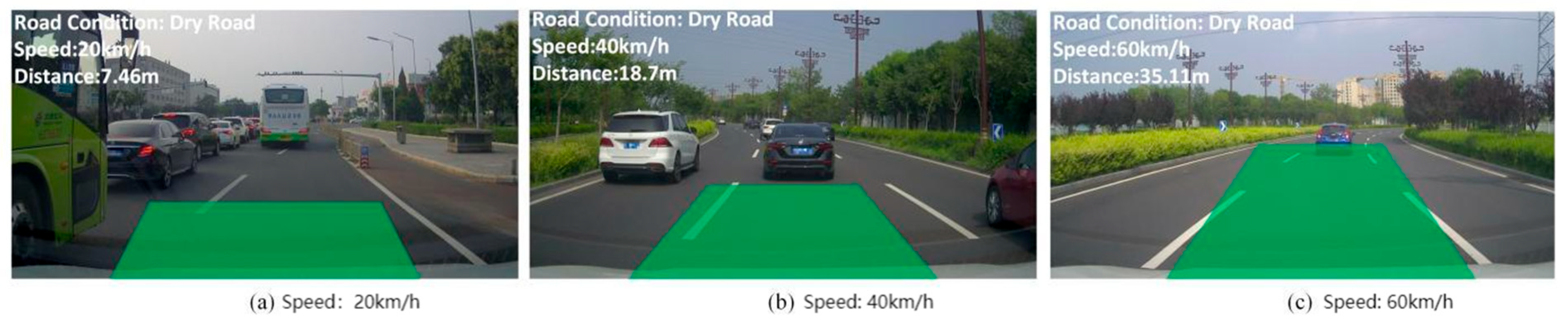
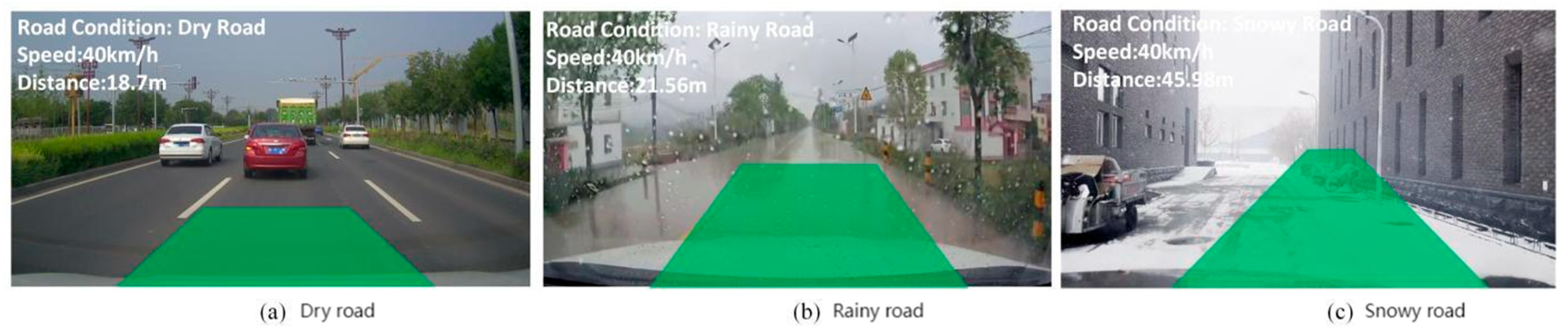
To verify the effectiveness of the adaptive safe distance model proposed in this paper, the algorithm was tested under different road conditions, and the experimental results are shown in Figure 11 and Figure 12. From Figure 11, when the ground is all dry asphalt pavement and the current speed is 20 km/h, the length of the dangerous area is 7.46 m; when the speed is 40 km/h, the length of the dangerous area is 18.7 m; when the speed is 60 km/h, the length of the dangerous area is 35.11 m; Figure 12 shows that at the same vehicle speed (40 km/h), when the road surface is dry, the length of the dangerous area is 18.7 m; when the road surface is wet after rain, the length of the dangerous area is 21.56 m; and when the road is snow-covered pavement, the length of the dangerous area is 45.98 m. These results demonstrate that the algorithm can construct an adaptive safe distance for collision warning under different vehicle speeds and road slippery states.

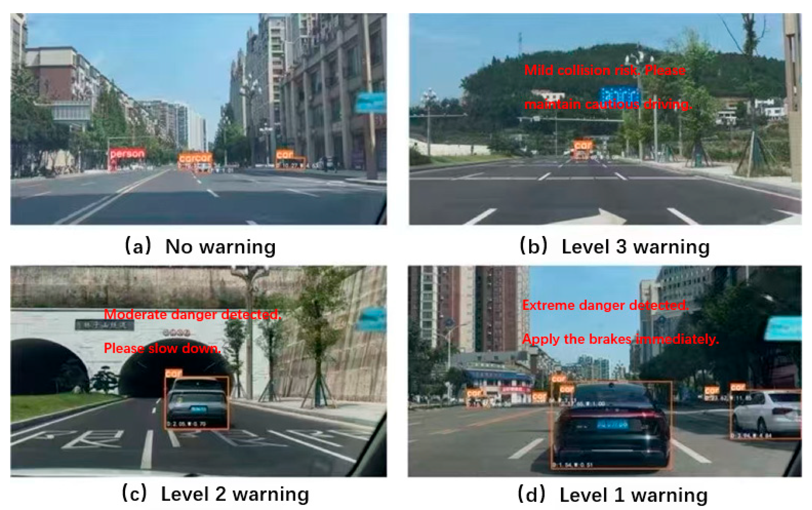
Finally, to verify the effectiveness of the proposed adaptive fusion collision warning strategy, a road section in the urban area was selected for real-vehicle experimental verification. The system recorded the current speed of this vehicle in real-time, and used a monocular camera to capture video for object detection. Partial output results of the collision warning system are shown in Figure 13. In Figure 13a, the vehicle speed is 42 km/h, the minimum safe braking distance is 8.59 m, and the longitudinal distance without a target is less than the minimum safe braking distance. At this time, the system did not issue a warning. In Figure 13b, the vehicle speed is 65 km/h, the minimum safe braking distance is 16.77 m, the longitudinal distance of the vehicle in front is 15.69 m, the relative speed between the two vehicles is 3.63 m/s, and the TTC is 4.32 s. The system classified this situation as a level-3 warning, prompting the driver to drive cautiously. In Figure 13c, the vehicle speed is 30 km/h, the minimum safe braking distance is 3.60 m, the longitudinal distance of the vehicle in front of the vehicle is 2.05 m, the relative speed between the two vehicles is 0.97 m/s, and the TTC is 2.12 s; the system classified this as a level-2 warning, advising the driver to slow down. In Figure 13d, the vehicle speed is 25 km/h, the minimum safe braking distance is 2.11 m, the longitudinal distance of the black car is 1.54 m, the relative speed between the two cars is 1.15 m/s, and the TTC is 1.34 s; at this time, the system classified this as a level-1 warning, prompting the driver to take immediate braking action.

To further verify the early warning effectiveness of the algorithm presented in this paper, a real-vehicle test was conducted on a specific section of a city road. The experimental procedure was conducted as follows: the time point at which the driver perceived a potential hazard and initiated braking action was recorded. At this moment, the ego vehicle’s speed was input into the warning system, and the time at which the system issued a warning was logged. The braking initiation time was then compared with the system warning time. If the difference between the two fell within 0.5 s, the warning was considered as a correct warning. If the system issued a warning but the driver did not perform braking, the event was classified as a false alarm. Conversely, if the driver executed braking while the system provided no warning, the case was recorded as a missed alarm. The accuracy rate, the error rate and no warning are introduced by three warning indicators. The results, compared with the traditional early warning algorithm [15], are shown in

Table 7. Comparative effects of different vehicle early warning systems.

Compared Strategies	Type of Warning	Level-1 Warning	Level-2 Warning	Level-3 Warning
	True Value	25	87	25
Traditional warning algorithm	False warning	7	4	8
	Correct warning	17	83	17
	No warning	1	0	0
Road states recognition integrated warning algorithm	False warning	3	3	2
	Correct warning	22	84	23
	No warning	0	0	0

.

The experimental results indicate that the accuracy rate of traditional warnings is 85.4%, a false alarm rate of 13.86% and a missed alarm rate of 0.73%; while the accuracy rate of the warning system proposed in this paper is 94.16%, a false alarm rate of 5.84% and no missed alarms. The overall accuracy rate has improved by 8.76%, and especially, the false alarm rate for predicting the level-1 warning and level-3 warning has decreased by 7.29% compared to traditional warnings [15]. This indicates that traditional TTC-based early warning strategies, due to their sensitivity to changes in relative vehicle speeds, often result in overly frequent or inaccurate warnings, especially during low-speed driving when early warnings are prone to occur prematurely. Therefore, this paper considers the impact of different road wetness conditions on the safe distance and the time-to-collision for early warnings, thereby further improving the accuracy of the warning zone model. Early warnings provide an extended temporal safety margin, enhancing collision avoidance potential especially under low-friction conditions. In this study, the driver’s braking action serves as the reference benchmark to ensure alert timeliness and actionability, thereby avoiding irrelevant alarms. Warnings issued more than 0.5 s before the driver’s reaction are recorded as valid early warnings, whose systematic optimization and evaluation will form a key focus of subsequent human–machine interaction research.

A Chi-squared test of independence was conducted on the outcome distributions (correct/false/missed alarm) from Table 7. The result (χ² = 12.47, df = 2, p = 0.002) confirms that the performance difference between the proposed and the traditional system is statistically significant at the 1% level. Further analysis using 95% confidence intervals (Wilson score method) underscores this improvement. The overall accuracy increased from 85.4% (CI: 78.5–90.5%) to 94.16% (CI: 88.9–97.0%), while the false alarm rate decreased from 13.86% (CI: 9.0–20.8%) to 5.84% (CI: 2.9–11.3%). The non-overlapping confidence intervals provide strong evidence for the significance of the enhancement.

5. Conclusions

This study developed an adaptive forward collision warning framework that dynamically adjusts safety margins based on real-time, vision-based recognition of road surface conditions. The core innovation integrates three synergistic components: (1) an ED-ResNet50 architecture incorporating grouped convolutions and hybrid attention mechanisms (ECA modules after Residual Blocks 2-3; DDS-DA after Block 4) substantially enhances road condition discrimination under adverse weather conditions; (2) synchronized YOLOv8-based vehicle detection enables dynamic calibration of safety distances and the time-to-collision through a friction-sensitive kinematic model that continuously adjusts warning thresholds according to instantaneous velocity and quantified road slipperiness; and (3) embedded real-vehicle validation confirms operational efficacy, demonstrating an 8.76% improvement in warning accuracy and 7.29% reduction in lateral and early false alarms versus static-threshold systems.

By fundamentally bridging the perception–decision gap through environment-responsive adaptation, this methodology delivers significant advancements in collision avoidance reliability during inclement weather, effectively mitigating accident risks through separating the task of visual appearance understanding from complex physical parameter regression. While this study demonstrates the effectiveness of the proposed framework under common adverse conditions, several limitations warrant consideration for real-world deployment. The performance of the vision-based recognition module remains susceptible to extreme lighting and occlusion, and the static mapping from visual class to friction coefficient may not capture real-time pavement dynamics. Future work will prioritize enhancing environmental robustness through sensor fusion, enabling online friction estimation by integrating vehicle dynamics, and extending the scenario coverage to include vulnerable road users and extreme low-friction hazards [43]. These advancements are essential for transitioning the system from controlled validation to reliable, all-weather operational support.

References

1. National Highway Traffic Safety Administration. Advancing Safety on America’s Roads; US Department of Transportation: Washington, DC, USA, 2015.
2. Xia, C. Research on a Vehicle Forward Collision Warning System Based on Monocular Vision. Master’s Thesis, Chongqing University, Chongqing, China, 2021. [Google Scholar]
3. Chen, T.; Liu, K.; Wang, Z.; Deng, G.; Chen, B. Vehicle forward collision warning algorithm based on road friction. Transp. Res. Part D Transp. Environ. 2019, 66, 49–57. [Google Scholar] [CrossRef]
4. Shojaeefard, M.H.; Mollajafari, M.; Ebrahimi-Nejad, S.; Tayebi, S. Weather-aware fuzzy adaptive cruise control: Dynamic reference signal design. Comput. Electr. Eng. 2023, 110, 108903. [Google Scholar] [CrossRef]
5. Chen, Y.; Zhang, P.; Wang, S.; Gong, D. Image Feature Based Machine Learning Approach for Road Terrain Classification. In 2018 TEEE International Conference on Mechatronics and Automation(ICMA); IEEE: New York, NY, USA, 2018; pp. 2097–2102. [Google Scholar]
6. Gui, Q.X.; Wang, G.; Wang, L.; Cheng, J.; Fang, H. Road surface state recognition using deep convolution network on the low-power-consumption embedded device. Microprocess. Microsyst. 2023, 96, 104740. [Google Scholar] [CrossRef]
7. Chen, S.J.; Liu, P.Y.; Bai, Y.B.; Wang, T.; Yuan, J. Computer vision based on high-speed pavement condition detection method. Meas. Control. Technol. 2023, 42, 44–51. [Google Scholar]
8. Yang, L.M.; Huang, D.Q.; Wei, X.; Wang, J. Deep learning-based identification of slippery state of road surface. Mod. Electron. Tech. 2022, 45, 137–142. [Google Scholar]
9. Wang, Z.; Wan, Q.; Qin, Y.; Fan, S.; Xiao, Z. Research on intelligent algorithm for alerting vehicle impact based on multi-agent deep reinforcement learning. J. Ambient. Intell. Humaniz. Comput. 2021, 12, 1337–1347. [Google Scholar] [CrossRef]
10. Das, S.; Maurya, A.K. Defining time-to-collision thresholds by the type of lead vehicle in non-lane-based traffic environments. IEEE Trans. Intell. Transp. Syst. 2019, 21, 4972–4982. [Google Scholar] [CrossRef]
11. Zhang, Y.; Hu, Y.; Hu, X.; Qin, Y.; Wang, Z.; Dong, M.; Hashemi, E. Adaptive Crash-Avoidance Predictive Control Under Multi-Vehicle Dynamic Environment for Intelligent Vehicles. IEEE Trans. Intell. Veh. 2024, 9, 7165–7175. [Google Scholar] [CrossRef]
12. Cai, C.X.; Gao, S.B.; Zhou, J.; Huang, Z.H. Freeway anti-collision warning algorithm based on vehicle-road visual collaboration. J. Image Graph. 2020, 25, 1649–1657. [Google Scholar]
13. He, Y. A Front Car Cut-in Prediction and Decision Control Method: CN202211168920.5. CN115384551A, 16 August 2025. [Google Scholar]
14. Hiraoka, T.; Takada, S. Improvement of evaluation indices for rear-end collision risk. IEEE Trans. Hum. Mach. Syst. 2017, 48, 102–109. [Google Scholar] [CrossRef]
15. Shen, H.Y.; Huo, K.; Wang, D.X. Research on Vehicle Collision Early Warning Algorithm Based on Machine Vision and Deep Learning. J. Shanxi Univ. (Nat. Sci. Ed.) 2023, 46, 617–627. [Google Scholar]
16. Zhu, B.; Piao, Q.; Zhao, J.; Wu, J.; Deng, W.W. Vehicle Longitudinal Collision Warning Strategy Based on Road Adhesive Coefficient Estimation. Automot. Eng. 2016, 38, 7. [Google Scholar] [CrossRef]
17. Pan, G.P.; Muresan, M.; Yu, R.; Fu, L. Real-time winter road surface condition monitoring using an improved residual CNN. Can. J. Civ. Eng. 2021, 48, 1215–1222. [Google Scholar] [CrossRef]
18. Marianingsih, S.; Widodo, W.; Pieter, M.S.S.; Manullang, E.V.; Nanlohy, H.Y. Machine Vision for the Various Road Surface Type Classification Based on Texture Feature. J. Mech. Eng. Sci. Technol. 2022, 6, 40–47. [Google Scholar] [CrossRef]
19. Dewangan, D.K.; Sahu, S.P. RCNet: Road classification convolutional neural networks for intelligent vehicle system. Intell. Serv. Robot. 2021, 14, 199–214. [Google Scholar] [CrossRef]
20. Huang, H.; You, Z.; Cai, H.; Xu, J.; Lin, D. Fast detection method for prostate cancer cells based on an integrated ResNet50 and YoloV5 framework. Comput. Methods Programs Biomed. 2022, 226, 107184. [Google Scholar] [CrossRef] [PubMed]
21. Zhao, X.; Wang, L.; Zhang, Y.; Han, X.; Deveci, M.; Parmar, M. A review of convolutional neural networks in computer vision. Artif Intell Rev. 2024, 57, 99. [Google Scholar] [CrossRef]
22. Li, J.; Wen, Y.; He, L. Scconv: Spatial and channel reconstruction convolution for feature redundancy. In Proceedings of the IEEE/CVF Conference on Computer Vision and Pattern Recognition, Vancouver, BC, Canada, 17–24 June 2023; pp. 6153–6162. [Google Scholar]
23. Burckhardt, M.; Eilert, G.; Freitag, R.; Mueller, A.; Schoeb, R.; Spiecker, R.; Kazan, S.; Zimmer, R. Process for Determination of Friction/Slip Characteristics of the Tires of a Road Vehicle and Slip Control System for Carrying Out the Process. U.S. Patent 5,599,076, 4 February 1997. [Google Scholar]
24. Girshick, R. Fast r-cnn. In Proceedings of the IEEE International Conference on Computer Vision, Santiago, Chile, 7–13 December 2015; pp. 1440–1448. [Google Scholar]
25. Ren, S.; He, K.; Girshick, R.; Sun, J. Faster R-CNN: Towards real-time object detection with region proposal networks. IEEE Trans. Pattern Anal. Mach. Intell. 2016, 39, 1137–1149. [Google Scholar] [CrossRef]
26. Durve, M.; Orsini, S.; Tiribocchi, A.; Montessori, A.; Tucny, J.-M.; Lauricella, M.; Camposeo, A.; Pisignano, D.; Succi, S. Benchmarking YOLOv5 and YOLOv7 models with DeepSORT for droplet tracking applications. Eur. Phys. J. E 2023, 46, 32. [Google Scholar] [CrossRef]
27. Long, W.; Wang, Y.; Hu, L.; Zhang, J.; Zhang, C.; Jiang, L.; Xu, L. Triple Attention Mechanism with YOLOv5s for Fish Detection. Fishes 2024, 9, 151. [Google Scholar] [CrossRef]
28. Varghese, R.; Sambath, M. YOLOv8: A Novel Object Detection Algorithm with Enhanced Performance and Robustness. In 2024 International Conference on Advances in Data Engineering and Intelligent Computing Systems (ADICS); IEEE: New York, NY, USA, 2024; pp. 1–6. [Google Scholar]
29. Al Riza, D.F.; Tulsi, A.A.; Momin, A. Assessing cacao beans fermentation degree with improved YOLOv8 instance segmentation. Comput. Electron. Agric. 2024, 227, 109507. [Google Scholar] [CrossRef]
30. Stein, G.P.; Mano, O.; Shashua, A. Vision-based ACC with a single camera: Bounds on range and range rate accuracy. In IEEE IV2003 Intelligent Vehicles Symposium. Proceedings (Cat. No. 03TH8683); IEEE: New York, NY, USA, 2003; pp. 120–125. [Google Scholar]
31. Hongshe, D.; Chongzhao, H.; Zhansheng, D. Determination of distance for vehicle collision avoidance warning and braking. J. Chang. Univ. (Nat. Sci. Ed.) 2002, 22, 89–91. [Google Scholar]
32. Lee, D.H.; Kim, S.K.; Kim, C.S.; Huh, K.S. Development of an autonomous braking system using the predicted stopping distance. Int. J. Automot. Technol. 2014, 15, 341–346. [Google Scholar] [CrossRef]
33. Zhang, Z. A flexible new technique for camera calibration. IEEE Trans. Pattern Anal. Mach. Intell. 2000, 22, 1330–1334. [Google Scholar] [CrossRef]
34. Maddern, W.; Pascoe, G.; Linegar, C.; Newman, P. 1 year, 1000 km: The Oxford RobotCar dataset. Int. J. Robot. Res. 2017, 36, 3–15. [Google Scholar] [CrossRef]
35. Geiger, A.; Lenz, P.; Stiller, C.; Urtasun, R. Vision meeFS-robotics: The KITTI dataset. Int. J. Robot. Res. 2013, 32, 1231–1237. [Google Scholar] [CrossRef]
36. Yu, F.; Chen, H.F.; Wang, X.; Xian, W.; Chen, Y.; Liu, F.; Madhavan, V.; Darrell, T. BDD100K: A diverse driving dataset for heter-ogeneous multitask learning. arXiv 2018, arXiv:1805.04687. [Google Scholar]
37. Szegedy, C.; Liu, W.; Jia, Y.; Sermanet, P.; Reed, S.; Anguelov, D.; Erhan, D.; Vanhoucke, V.; Rabinovich, A. Going deeper with convolutions. In Proceedings of the IEEE Conference on Computer Vision and Pattern Recognition, Boston, MA, USA, 7–12 June 2015; pp. 1–9. [Google Scholar]
38. Szegedy, C.; Vanhoucke, V.; Ioffe, S.; Shlens, J.; Wojna, Z. Rethinking the inception architecture for computer vision. In Proceedings of the IEEE Conference on Computer Vision and Pattern Recognition, Las Vegas, NV, USA, 27–30 June 2016; pp. 2818–2826. [Google Scholar]
39. Yang, W.; Huang, L.H.; Qu, X.L. Dual Attention Network for the Classification of Road Surface Conditions Based on EfficientNet. J. Mech. Eng. 2022, 58, 211–222. [Google Scholar]
40. Howard, A.G.; Zhu, M.; Chen, B.; Kalenichenko, D.; Wang, W.; Weyand, T.; Andreetto, M.; Adam, H. MobileNets: Efficient convolutional neural networks for mobile vision applications. arXiv 2017, arXiv:1704.04861. [Google Scholar]
41. Huang, G.; Liu, Z.; Van Der Maaten, L.; Weinberger, K.Q. Densely connected convolutional networks. In Proceedings of the IEEE Conference on Computer Vision and Pattern Recognition, Honolulu, HI, USA, 21–26 July 2017; pp. 4700–4708. [Google Scholar]
42. He, K.; Zhang, X.; Ren, S.; Sun, J. Deep residual learning for image recognition. In Proceedings of the IEEE Conference On Computer Vision and Pattern Recognition, Las Vegas, NV, USA, 27–30 June 2016; pp. 770–778. [Google Scholar]
43. Zhang, Y.; Tang, X.; Qin, Y.; Dong, M. DMIC: Decision-Making Integrated Predictive Control for Intelligent Vehicles. IEEE Trans. Syst. Man Cybern. Syst. 2025, 55, 6312–6324. [Google Scholar] [CrossRef]
Figure 1. The framework of the road slippery states-aware adaptive collision warning method for IVs.
Electronics 15 00829 g001
Figure 2. The framework structure of ED-ResNet50 model.
Electronics 15 00829 g002
Figure 3. ECA module structure diagram.
Electronics 15 00829 g003
Figure 4. The process of Dilated Depthwise Separable Convolution.
Electronics 15 00829 g004
Figure 5. The structure of the Dual Attention Module.
Electronics 15 00829 g005
Figure 6. The operation of grouped convolution.
Electronics 15 00829 g006
Figure 7. Yolov8 model structure.
Electronics 15 00829 g007
Figure 8. The process of the adaptive multi-level early warning strategy considering the road slippery states.
Electronics 15 00829 g008
Figure 9. The experiment platform and driving scene.
Electronics 15 00829 g009
Figure 10. Road dataset samples.
Electronics 15 00829 g010
Figure 11. Schematic diagram of danger zones at speeds of 20 km/h (a), 40 km/h (b) and 60 km/h (c) with all dry asphalt pavement.
Electronics 15 00829 g011
Figure 12. Schematic diagram of dangerous areas for different road slippery states.
Electronics 15 00829 g012
Figure 13. Partial output results of the collision warning system.
Electronics 15 00829 g013