


Abstract
Reliability testing for Single Event Effects (SEEs) requires accurate localization of heavy-ion tracks from projection images. Conventional localization often relies on handcrafted features and geometric fitting, which is sensitive to noise and difficult to accelerate in hardware. This paper presents a lightweight detector based on YOLOv5n that treats charge tracks in Topmetal pixel sensor projections as distinct objects and directly regresses the track angle and intercept, along with bounding boxes, in a single forward pass. On a synthetic dataset, the model achieves a precision of 0.9626 and a recall of 0.9493, with line-parameter errors of 0.3930° in angle and 0.4842 pixels in intercept. On experimental krypton beam data, the detector reaches a precision of 0.92 and a recall of 0.96, with a position resolution of 52.05 μm. We further deploy the model on an Xilinx Alveo U200, achieving an average per-frame accelerator latency of 3.1 ms while preserving measurement quality. This approach enables accurate, online track localization for SEE monitoring on Field-Programmable Gate Array (FPGA) platforms.
1. Introduction
Single Event Effect (SEE) refers to a phenomenon in which high-energy charged particles in a radiation environment strike sensitive regions of microelectronic devices, causing abnormal logic states or functional failures [1]. With the increasing use of high-performance microelectronics and large-scale integration in spacecraft, aircraft, and missile systems, the risk associated with SEEs has become more serious [2,3,4]. The key to enhancing the radiation resistance of electronic devices lies in rapidly and accurately locating their sensitive regions to SEEs, thereby enabling targeted, radiation-hardened design. Therefore, achieving efficient and rapid detection of SEE and localization of sensitive regions has become a critical problem that urgently needs to be addressed in the radiation-hardened design of electronic equipment for aerospace, military, and other fields [5,6,7,8].
Silicon pixel detectors are two-dimensional readout detectors composed of numerous small-area sheet-like electrodes. Due to their small pixel size, typically tens of micrometers, they offer extremely high spatial resolution and can be used as a beam localization detector [9,10]. A beam localization detector can track the beam particles, allowing the localization of regions where SEEs occur by identifying these tracks. Previous research utilized a beam localization detector based on the Topmetal silicon pixel chip [11]. By employing track reconstruction algorithms to analyze the projection paths of heavy ions, it becomes possible to precisely locate the impact positions of each heavy ion that triggered a SEE on the tested integrated circuit. This beam localization detector is non-intercepting [12,13,14] and is capable of measuring beam profiles, positions, intensities, and other parameters in real time without interfering with, intercepting, or attenuating the beam [15]. This measurement process generates a large volume of data. Storing this data offline would consume significant storage space, necessitating the use of online track localization algorithms to process experimental data in real time, thereby alleviating the system pressure on data transmission and storage.
Traditional track localization often uses geometric model fitting, such as the Hough transform and random sample consensus (RANSAC), which detect lines by voting in parameter space or random sampling [16,17]. These pipelines depend on edge extraction and thresholds. Their stability degrades under changing backgrounds and realistic sensor artifacts. Deep neural networks have been explored for particle physics and track reconstruction from detector readouts [18,19]. FPGA-based inference has also been reported in particle physics systems to achieve fixed low latency for online processing [20]. Most existing learning-based approaches focus on intermediate tasks such as detection, segmentation, or classification, and the final track parameters are obtained by post-processing. High-accuracy models are often large and are evaluated on GPUs in offline workflows.
This work is motivated by the need for a lightweight one-stage detector that is practical for FPGA deployment in an online SEE monitoring setting. We adopt a You Only Look Once (YOLO) formulation because it performs classification and localization in a single forward pass, which fits low-latency streaming requirements [21]. From cost and performance perspectives, our goal is to use a model that is sufficiently accurate for track localization while remaining compact enough for efficient hardware deployment. We therefore build on the YOLOv5n family, which offers a favorable balance between detection accuracy and computational complexity [22]. In our task, YOLOv5n already provides reliable localization performance, and its lightweight design reduces computation, memory traffic, and hardware resource demand, which directly benefits real-time streaming inference. In contrast, larger backbones can achieve higher accuracy across general vision benchmarks. However, their increased model size and compute requirements typically lead to higher deployment costs and reduced efficiency for online processing. Accordingly, we focus on a compact YOLOv5n-based design and tailor it to heavy-ion track projections to enable real-time inference and direct extraction of physically meaningful track information under hardware acceleration [23].
2. Methodology
2.1. YOLO-Based Principle for Particle Track Projection Localization
After pedestal subtraction and basic denoising, each projection on a given anode plane can be regarded as a grayscale image of size pixels, where slender bright bands correspond to charged particle track projections embedded in a stochastic background. Let denote pixel coordinates in this image. Each visible track projection is well approximated by a straight line
where k is the slope and b is the intercept at the left boundary . For downstream analysis, it is more convenient to parameterize the line by its angle with respect to the horizontal axis and the same intercept b, with
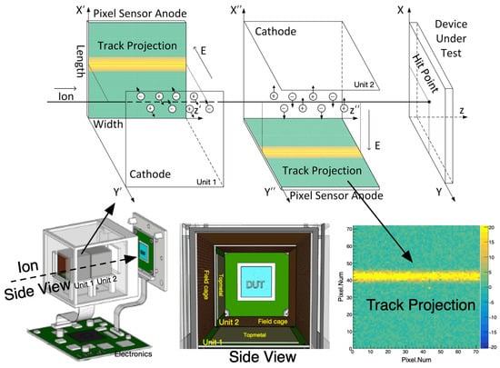
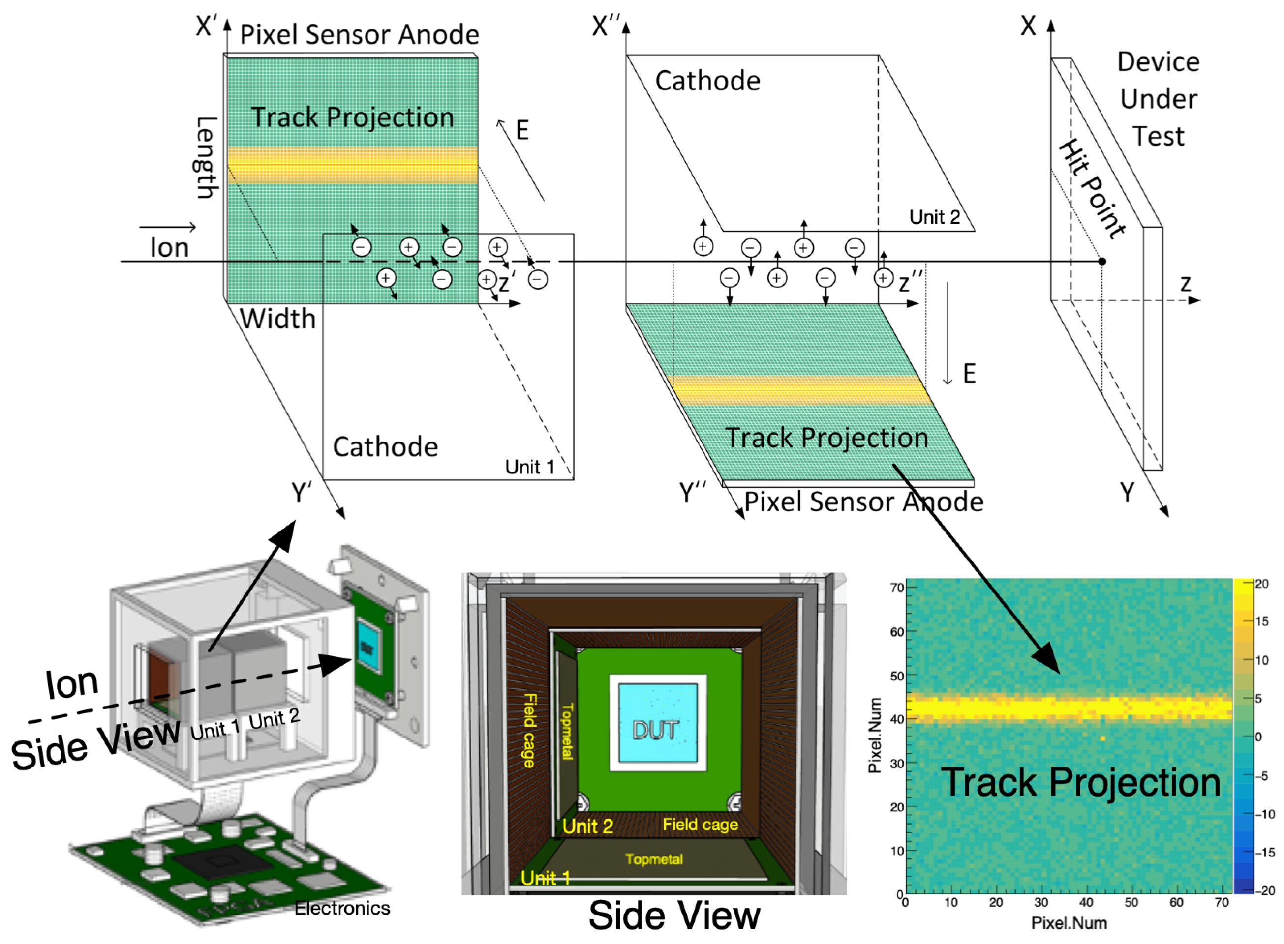
The pair is physically interpretable, compact, and directly related to the ion incident direction and the effective hit position on the device under test. The detector principle is illustrated in Figure 1.
Figure 1.
Principle of the Topmetal-based beam tracking detector and an example of a single heavy-ion projection. Two orthogonal drift cells with uniform electric fields guide electrons to pixel anodes and form projections on the X–Z and Y–Z planes. These projections are used to localize the impact position on the device under test in the online pipeline. Arrows indicate the electric-field direction, and dashed lines denote the ion beam path and auxiliary reference lines for localization.
The key idea of the proposed approach is to let a YOLO-based detector infer these line parameters directly from the projection image. Each track projection is treated as a thin object that needs to be detected and described by a small set of geometric parameters. Instead of relying on handcrafted edge detection and Hough [24,25] or RANSAC fitting [26], the detector learns to identify all track segments in a frame and to regress their angles and intercepts in a single forward pass. Conceptually, the network views the projection as a grid of candidate locations, evaluates at each location whether a track passes through the corresponding receptive field, and, if so, outputs the position and line parameters of the track segment.
Given an input frame, the desired output of the YOLO-based model is therefore a set of line parameter tuples
where N is the number of visible tracks in the frame, and denote the angle and intercept of the i-th track in the original sensor coordinate system, and is a confidence score. Coarse bounding boxes are also retained for each track to describe the spatial extent of the projection and assist in visualization.
In this work, YOLOv5n serves as a compact and efficient backbone for implementing the above principle and offers a favorable balance between detection accuracy and computational cost [27,28,29]. It can process each projection image with very low latency, which is essential for online SEE monitoring. Its fully convolutional structure and fixed computation graph are naturally aligned with a streaming Field-Programmable Gate Array (FPGA) implementation, where weights can be quantized and intermediate feature maps can be buffered on chip. At the same time, the mature training pipeline and anchor-based design of YOLOv5n make it straightforward to adapt the detector from generic natural images to the highly structured and nearly linear patterns that appear in heavy ion track projections.
2.2. YOLO-Based Detection Architecture
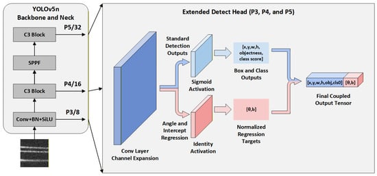
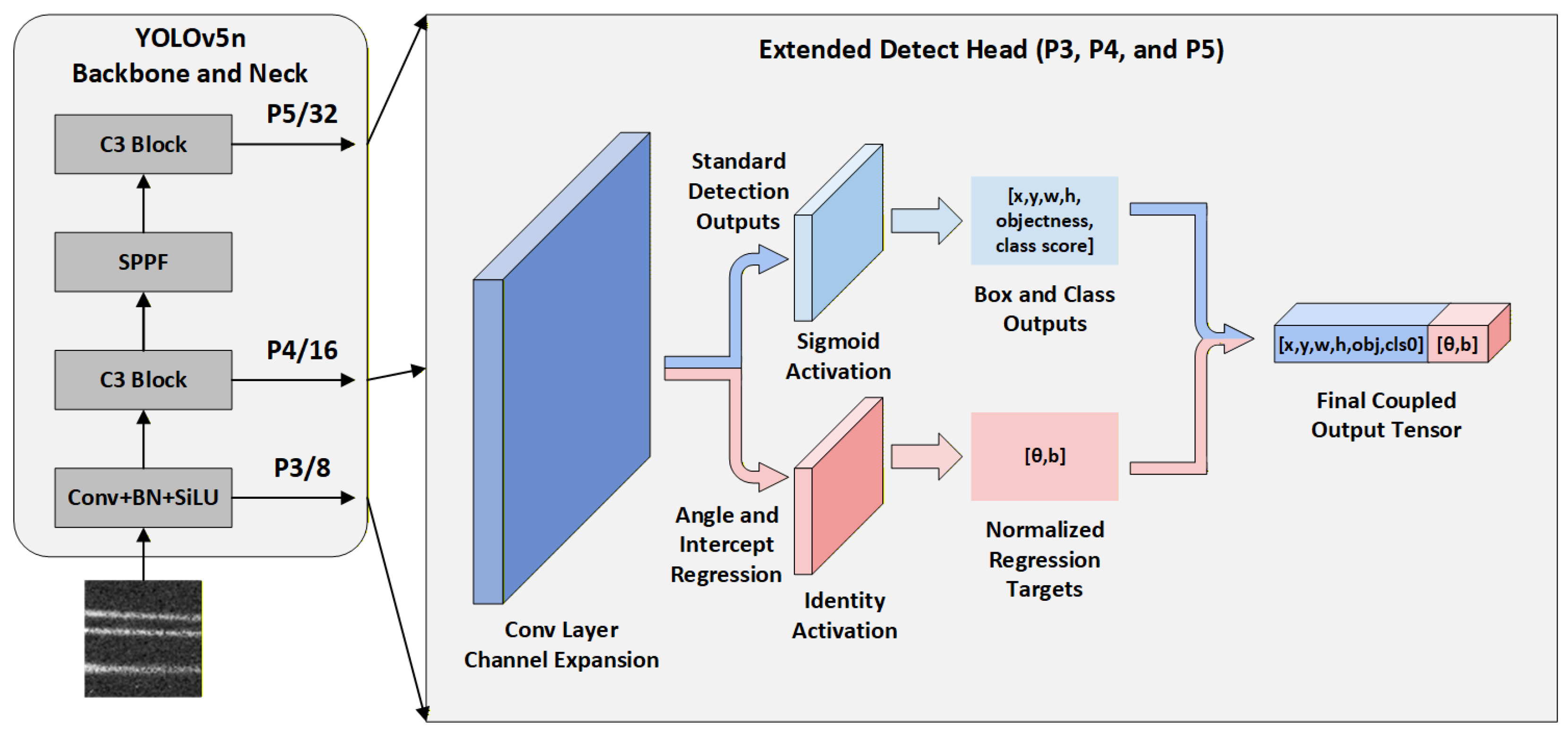
The core of the proposed method is a detector that utilizes an architecture similar to YOLOv5n and is tailored to track projections. The input to the network is a single channel frame obtained from one projection plane of the detector. Before entering the backbone, this frame is resized to and then replicated across three channels, yielding a tensor that is compatible with the standard YOLOv5n input format and pretrained convolutional kernels. As illustrated in Figure 2, the replicated tensor is processed by a compact convolutional backbone and feature pyramid. It is transformed into three feature maps at strides 8, 16, and 32, with spatial sizes , , and , respectively.
Figure 2.
Schematic of the YOLOv5n-based model used in this work. The detection head is extended with an additional regression branch to output normalized line parameters alongside standard bounding box predictions. Blue denotes the standard detection branch for box and class outputs, while pink denotes the added regression branch for angle and intercept.
Starting from the YOLOv5n design, we construct a variant that is explicitly tailored to the characteristics of projection images and to the requirement of precise line parameter estimation. The backbone, together with the feature pyramid network and the path aggregation network style neck, is configured for a small field of view, producing three prediction scales that jointly capture short, nearly straight local segments as well as longer tracks that approach the edges of the sensor. This configuration preserves the efficiency of YOLOv5n, while specializing the network to the limited spatial extent and low texture complexity of projection track patterns.
The detection head follows the general structure of YOLOv5 but is extended to regress line parameters in addition to bounding boxes. For each spatial location and anchor on each detection scale, the head outputs an 8-dimensional prediction vector
where are the normalized center coordinates of the bounding box, are its normalized width and height, o is the objectness score indicating the presence of a track, c is the class logit, and are the normalized line parameters. Since the task involves only one semantic class, the classification branch is not optimized during training (i.e., the classification loss is disabled), and the final detection confidence is determined solely by the objectness score o.
During inference, the predicted bounding box parameters from all three detection scales are decoded in the usual YOLO manner and converted back to the original pixel coordinates of the projection image. Candidate boxes from the three scales are merged, and Non-Maximum Suppression (NMS) is applied to suppress overlaps and retain a compact set of high confidence track candidates. For each remaining detection, the corresponding normalized line parameters are denormalized to obtain the physical angle and intercept b of the track in the sensor plane.
In summary, this customized model serves as an end-to-end measurement model for track geometry: a single projection image is directly mapped to a set of track instances, parameterized by their angles and intercepts. This enables the network to learn object localization and line regression jointly, producing the desired physical parameters and b without a separate fitting stage.
2.3. Joint Loss for Detection and Line Parameter Regression
Training the detector requires supervision of both bounding box localization and line parameter regression. For each ground truth track in a frame, the synthetic dataset provides a bounding box and the corresponding angle and intercept in the coordinate system. The line parameters are normalized before they are used as regression targets. Denoting the maximum absolute track angle in the synthetic data by and the image size by , the normalized targets are defined as
With this definition, both and lie approximately in the range . This keeps the regression losses for the line parameters on a scale comparable to the box loss, stabilizing training.
Let denote the set of positive predictions, namely those anchors that are assigned to ground truth tracks according to the standard YOLO matching strategy. For a prediction matched to ground truth , the network outputs
where are the decoded bounding box parameters, is the objectness score that reflects the confidence that anchor i covers a valid track, and are the predicted normalized line parameters. The corresponding target vector is
where denote the ground truth box parameters, and are the corresponding normalized line parameter targets. In our single class setting, the class target is constant and the classification loss is disabled. Therefore, only the objectness, box regression, and line parameter regression terms contribute to optimization.
The overall training objective combines the objectness loss, the bounding box regression loss, and the line parameter regression losses:
where , and are scalar weights that balance the different components. Note that the classification loss term is omitted because the task contains only one class and the corresponding branch is not optimized.
The objectness loss follows the standard YOLO formulation and is implemented as a binary cross entropy loss on for all anchors, including negatives. The box loss is computed over positive anchors using a Complete Intersection over Union (CIoU) loss between the predicted and ground truth boxes:
For the line parameters, we use Smooth- regression losses on the normalized targets:
The Smooth- loss provides stable gradients near the optimum while being less sensitive to outliers than the loss. These terms explicitly penalize errors in the angle and the intercept, and encourage the detector to learn geometrically accurate line parameters in addition to tight bounding boxes. The combined loss drives the network to discover slender track projections, regress their bounding boxes, and directly predict their normalized line parameters in a single training objective. During inference, the normalized outputs are denormalized back to , which yields an end-to-end mapping from raw projection frames to line parameters of charged particle tracks.
3. Experiments on Synthetic and Beam Test Data
3.1. Synthetic Dataset for Track Projections
To quantitatively evaluate the proposed detector, a synthetic dataset is constructed that mimics the heavy ion track projections recorded by the Topmetal-based beam tracking system. Each sample corresponds to a single projection frame on one anode plane and is represented as a grayscale image of size pixels. The gray level of each pixel reflects the collected charge on the corresponding pad, resulting in slender bright bands where charged particle tracks traverse the sensitive volume. At the same time, the remaining regions are dominated by stochastic electronic noise and baseline fluctuations.
The intensity model is based on the fundamental physics of charge deposition and diffusion in a gaseous drift cell. A heavy ion traversing the gas volume deposits energy along its track according to the stopping power. The deposited energy is converted into ionization electrons with a mean work function and is further reduced by an effective charge collection efficiency, which accounts for recombination and imperfect transport. The total number of electrons associated with a track is proportional to its physical length, the stopping power, and the collection efficiency. This electron yield is then mapped to the analog to digital converter values through a fixed conversion factor. In the simulator, the electrons are distributed along an ideal straight segment that represents the track projection on the anode plane. Each elemental cloud is broadened transversely by a Gaussian kernel whose width is set by the diffusion coefficient and the drift distance in the uniform electric field. The broadened charge distribution is accumulated on the image grid to form a frame. Independent Gaussian noise with zero mean and unit variance is added to every pixel to emulate residual electronic noise and pedestal fluctuations. Negative values are clipped, and a fixed gain factor is applied, so that the simulated frames exhibit elongated bands with realistic widths and intensity variations superimposed on a noisy background.
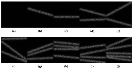
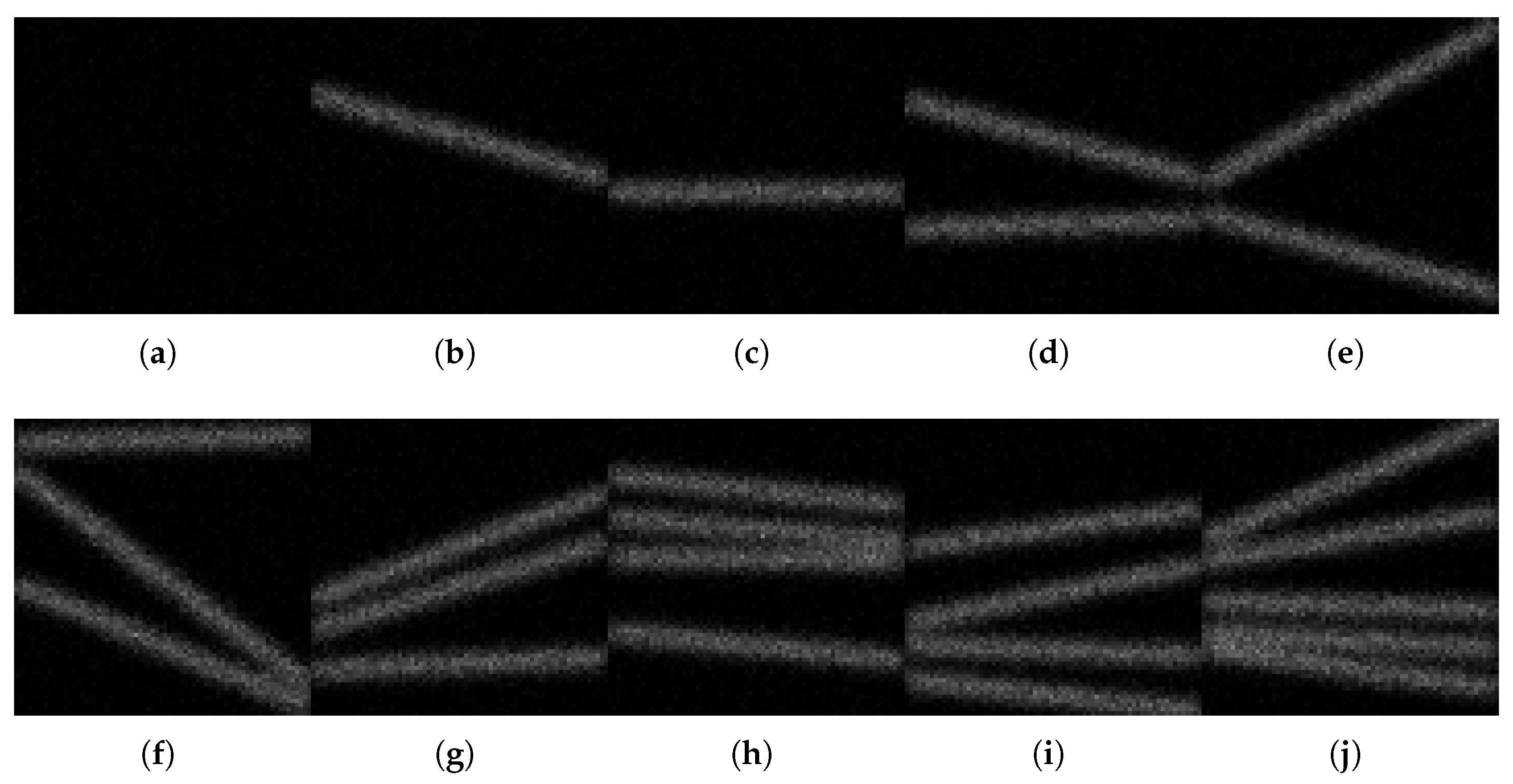
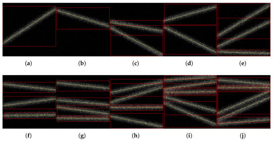
In each synthetic frame, the number of visible tracks is treated as a random variable that reflects the fluctuating multiplicity in real SEE tests. The track count is allowed to range from zero to five, with single-track and two-track configurations being the most frequent, and frames with more tracks occurring with progressively lower probability. Frames without any track serve as hard negatives, regularizing the detector and reducing false alarms. Meanwhile, frames with multiple tracks emulate crowded conditions in which several projections coexist in the same field of view. Figure 3 shows representative examples of purely noisy frames, frames containing a single track at different angles, and frames with multiple tracks that span different orientations and positions.
Figure 3.
Representative samples from the synthetic dataset. (a) background noisy frame; (b) single-track example 1; (c) single-track example 2; (d) two-track example 1; (e) two-track example 2; (f) three-track example 1; (g) three-track example 2; (h) four-track example 1; (i) four-track example 2; (j) five-track example.
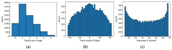
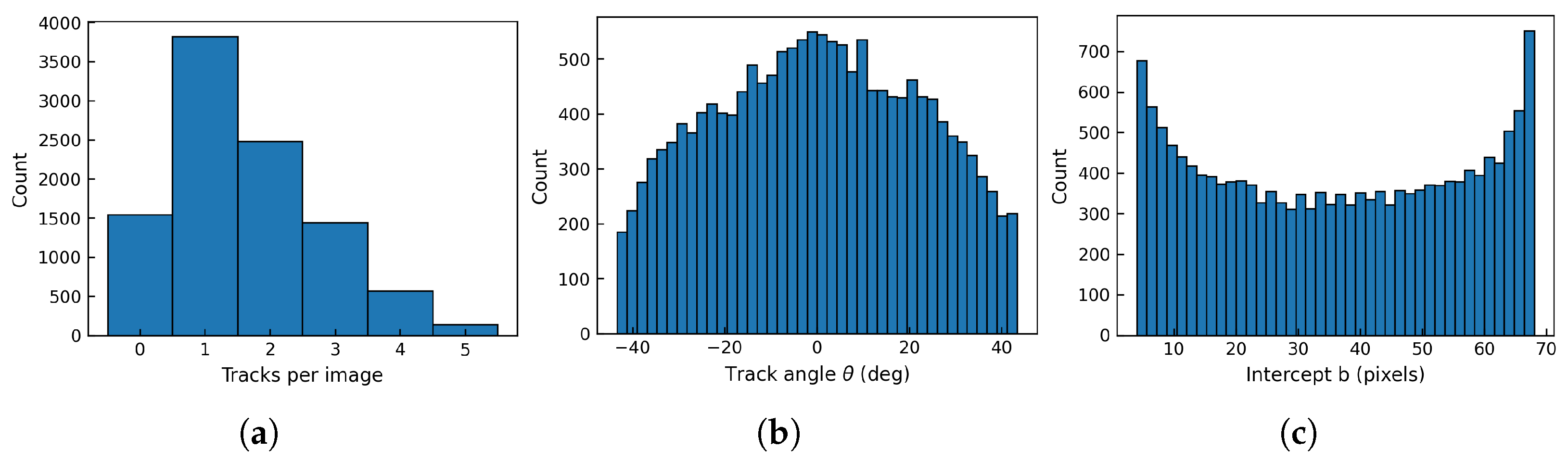
The geometric parameters of each track are specified by the angle and the intercept b at the left boundary of the image window. In the generator, the incident angle is drawn from a broad range so that both shallow and steep projections are represented. At the same time, the intercept b is sampled across the active vertical extent of the sensor. A small margin is reserved near the top and bottom edges to prevent tracks that only clip the corners, resulting in a negligible visible length. As a result, the synthetic dataset provides a balanced coverage of incident directions and hit positions that reflects the geometric constraints imposed by the detector layout. Figure 4 summarizes the resulting distributions of track angles and intercepts over the whole dataset. The angle histogram is close to uniform within the design range, and the intercept histogram is approximately flat in the central region, with a mild decline near the edges due to the active area margin.
Figure 4.
Distributions of track multiplicity and line parameters in the synthetic dataset. (a) Histogram of the number of tracks per frame; (b) histogram of the track angle in degrees; (c) histogram of the intercept b at the left boundary in pixel units.
For each simulated track, the generator records a bounding box that tightly encloses the broadened segment together with the underlying line parameters in the image coordinate system. All labels are stored in a unified YOLO-style format with seven entries per track , where are the normalized box center coordinates, are the normalized width and height, and the class index is fixed to zero for particle tracks. The normalized line parameters are defined as in (5) and serve as regression targets of the detector. Frames that do not contain any visible track yield empty label files, which act as hard negatives during training.
In total, 10,000 synthetic projection images are generated and randomly split into training, validation and test subsets with an 8:1:1 ratio.
3.2. Training and Evaluation on Synthetic Data
The network is trained by minimizing the multi-task loss L in (8), which combines objectness classification, bounding box regression, and direct regression of the line parameters. Optimization is carried out using stochastic gradient descent with momentum and weight decay. A standard YOLOv5 learning-rate schedule is adopted, with and a final LR factor , including a 3-epoch warm-up. The model is trained for 300 epochs with a batch size of 128. The initial learning rate is set to for the detection head and reduced for earlier layers following the standard YOLOv5n training recipe.
Data augmentation is applied with particular care, since the regression targets explicitly encode track geometry. Horizontal flipping is enabled, and the corresponding ground truth parameters are recomputed so that and remain consistent in the coordinate system after transformation. In contrast, spatial augmentations such as random rotation, scale jitter, mosaic, and perspective warping are disabled because they would alter the underlying line geometry and invalidate the parameter labels. Photometric perturbations are retained, as they preserve line structure while improving robustness to intensity variations in real beam projections. The main training and evaluation hyperparameters are summarized in Table 1.
Table 1.
Main training and evaluation hyperparameters on synthetic data.
With the above configuration, training converges stably. The multi-task loss decreases smoothly, and the validation performance follows the same trend, indicating that localization and geometric regression are learned in a balanced manner.
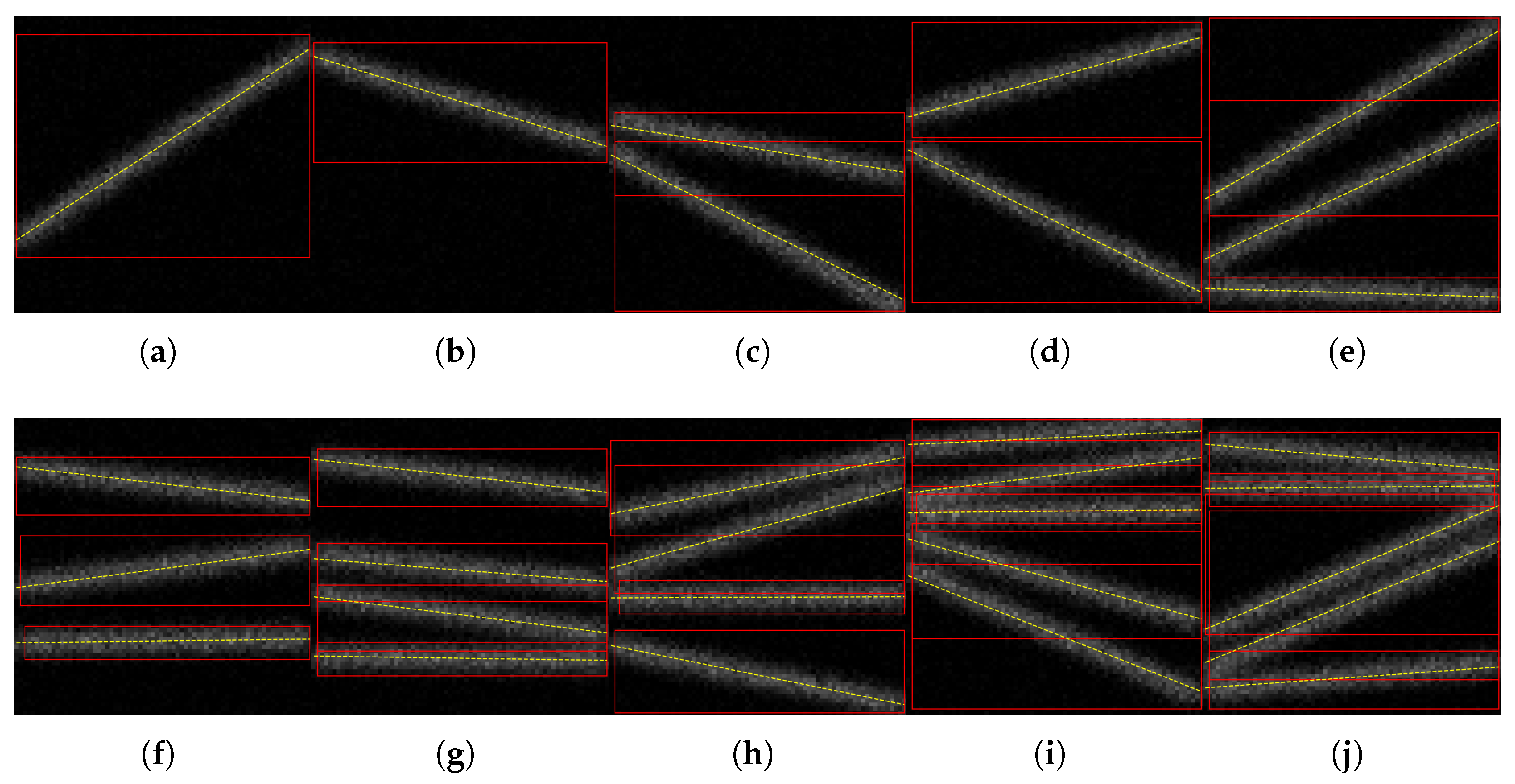
Figure 5 shows representative examples from the synthetic test set. The predicted bounding boxes and the regressed line parameters are overlaid on the input projections. As shown, the proposed model robustly localizes track candidates across different track configurations and reconstructs the corresponding line geometry with good visual consistency.
Figure 5.
Representative examples from the synthetic test set with overlaid predictions. The red boxes indicate the predicted track bounding boxes, and yellow lines indicate the regressed track lines. (a) single-track example 1; (b) single-track example 2; (c) two-track example 1; (d) two-track example 2; (e) three-track example 1; (f) three-track example 2; (g) four-track example 1; (h) four-track example 2; (i) five-track example 1; (j) five-track example 2.
Quantitative performance on the synthetic test set is evaluated using fixed confidence and NMS IoU thresholds. Table 2 summarizes the standard detection metrics of the proposed detector, together with the Mean Absolute Errors (MAEs) of the regressed angle and intercept. For a set of N matched tracks, the angle and intercept MAEs are computed as
where are the line parameters predicted by the network and are the corresponding reference values in the synthetic test set.
Table 2.
Performance comparison on the synthetic test set.
For comparison, we evaluate two classical fitting-based baselines, a Hough detector and an RANSAC-based line fitter, and a modern lightweight detector, YOLOv8n, on the same synthetic test set. Hough and RANSAC output line hypotheses rather than bounding boxes. Precision and recall are computed at the track level under the same matching protocol. The MAEs of the angle and intercept quantify geometric accuracy. YOLOv8n produces bounding boxes. The line parameters are obtained by applying an RANSAC line fit within each predicted ROI, yielding consistent evaluations of across all methods.
Table 2 summarizes the results. The proposed model achieves a precision of 0.9626 and a recall of 0.9493. Direct parameter regression yields MAEs of 0.3930° for the angle and 0.4842 pixels for the intercept. The Hough baseline achieves a recall of 0.9427 but has a lower precision of 0.9024. The geometric errors increase to 1.0035° and 2.6094 pixels, consistent with over-detection under noisy backgrounds. RANSAC provides strong detection and improved geometry, with a precision of 0.9436, a recall of 0.9584, an angle MAE of 0.4135°, and an intercept MAE of 0.6013 pixels. The proposed model remains more accurate in parameter estimation. YOLOv8n attains a precision of 0.9952 and a recall of 0.9938, while the recovered parameters show larger errors of 2.5371° and 3.1593 pixels. YOLOv8n is optimized for bounding box localization. The subsequent ROI-based RANSAC fitting is sensitive to slight localization bias and background residuals, which degrade the recovered line parameters.
We further evaluate robustness on the synthetic test set by injecting additive white Gaussian noise into the input frames to achieve controlled Signal-to-Noise Ratio (SNR) levels. Table 3 reports track-level precision, recall, and the MAE of the estimated line parameters on matched true positives.
Table 3.
Robustness evaluation under additive noise with different SNR levels on the synthetic test set.
The results show stable performance above 25 dB. Precision and recall remain above 0.93. The angle MAE remains below 0.67 degrees. The intercept MAE remains below 0.74 pixels. As SNR decreases further, detection performance degrades gradually. Precision and recall drop to about 0.90 at 20 dB and to about 0.88 at 15 dB. At 10 dB, the method still maintains a precision of 0.8186 and a recall of 0.8111. The overall trend indicates a clear operating range, with reliable localization at moderate SNR and a graceful degradation pattern under severe noise.
3.3. Ablation Studies
We conduct ablation experiments to examine key design choices of the proposed detector, including the regression branch, the input channel representation, the backbone capacity, and the regression loss weight. Table 4 reports the results. Precision and recall are computed using a track-level matching protocol at an IoU of 0.50. The mean Average Precision (mAP)@0.5 metric is obtained from the official YOLOv5 evaluation routine. The quantities MAE and MAE b are the MAEs of the regressed line angle and intercept on matched true positives.
Table 4.
Ablation studies of key design choices.
The baseline configuration achieves high detection accuracy and stable parameter regression. When the regression branch is removed, we estimate the line parameters by applying a RANSAC-based fitting procedure to the detected candidate boxes. The detection metrics remain comparable, whereas the parameter accuracy degrades substantially. This result suggests that post hoc geometric fitting within candidate boxes is unreliable in our setting, likely because multiple tracks may coexist within a single detected box, leading to ambiguous inlier sets and compromising robust line fitting.
We further evaluate the input channel representation by replacing the replicated three-channel input with a single-channel input. The performance remains comparable across detection metrics and regression errors. For practical implementation, we retain the replicated three-channel input in the final system to maintain compatibility with the standard YOLOv5 input interface and pretrained weights. Since the replicated channels do not add information and the additional computation is limited to the first convolutional layer, this choice has a negligible impact on overall inference latency.
To investigate model capacity, we replaced the YOLOv5n backbone with the larger YOLOv5s, while detection accuracy remains high, regression errors increase significantly. This suggests that simply increasing model size does not benefit line parameter estimation in our sparse feature setting and may lead to optimization difficulties. Finally, we analyzed the regression loss weight. Increasing the weight from 1.0 to the baseline value of 5.0 significantly improves accuracy, whereas further increases to 10.0 yield diminishing returns. This indicates that balancing the regression objective is critical for optimal parameter estimation.
Overall, these ablations show that end-to-end regression and proper loss weighting are the main contributors to accurate track localization. At the same time, input channel replication and backbone scaling have only a limited impact on performance in our setting.
3.4. Evaluation on Real Beam Test Data
To verify that the detector generalizes beyond the synthetic domain, it is further evaluated on projection frames acquired during a dedicated heavy-ion beam test. The experiment for the beam tracking prototype detector was carried out at the Heavy Ion Research Facility in Lanzhou (HIRFL). The detector utilizes a pixel chip named Topmetal, which features a pixel array with a pixel pitch of 83 μm. During the test, a krypton ion beam with an energy of 25 MeV/u and a spot size of 5.29 cm2 was delivered in ambient air at room temperature, and the pixel chip recorded the tracks of the incident ions.
The raw readout frames from the Topmetal chip are processed by the same front end chain as used in the online SEE monitoring system. This chain includes pedestal subtraction, removal of obviously saturated or dead channels, and basic noise suppression. After this preprocessing, the charge distribution on each anode plane is cropped and grayscale. In contrast to the idealized simulations, these real frames contain effects such as gain non-uniformity across the array, occasional hot pixels, and fluctuations in the beam profile, thereby providing a realistic test of the detector’s robustness.
We evaluate the synthetically trained network on real data, using identical detection settings. To establish ground truth, we manually labeled 149 frames. For each track, we annotated the two endpoints of the visible bright segment. These endpoints were used to generate a tightly enclosing bounding box and to compute the line parameters within the coordinate system. Performance is assessed via standard metrics by matching predictions to ground truth. Additionally, spatial consistency is quantified by position resolution, defined as the root mean square of the perpendicular distances between the reference track and the predicted line.
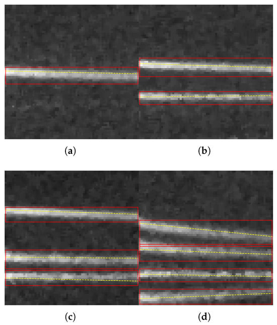
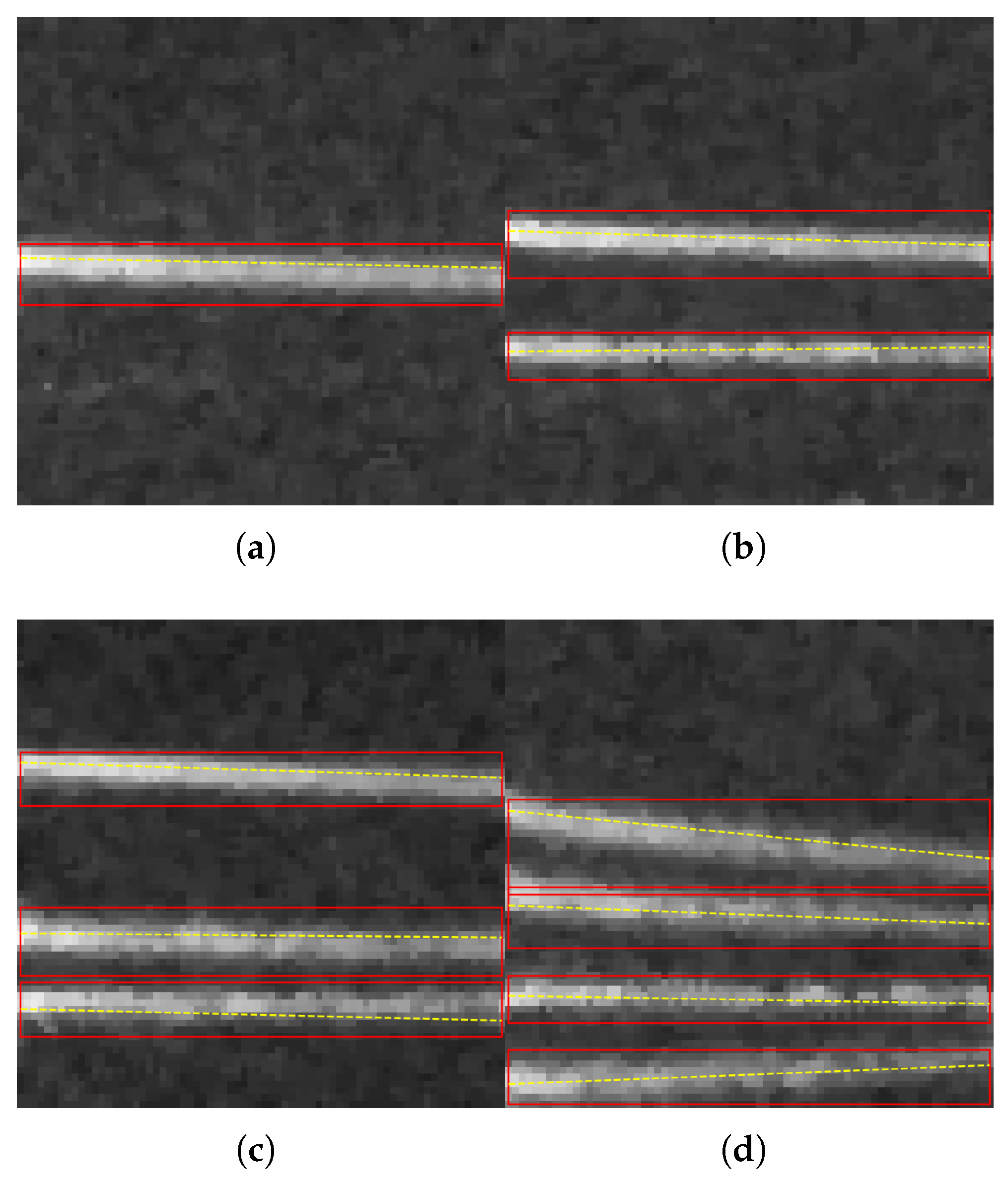
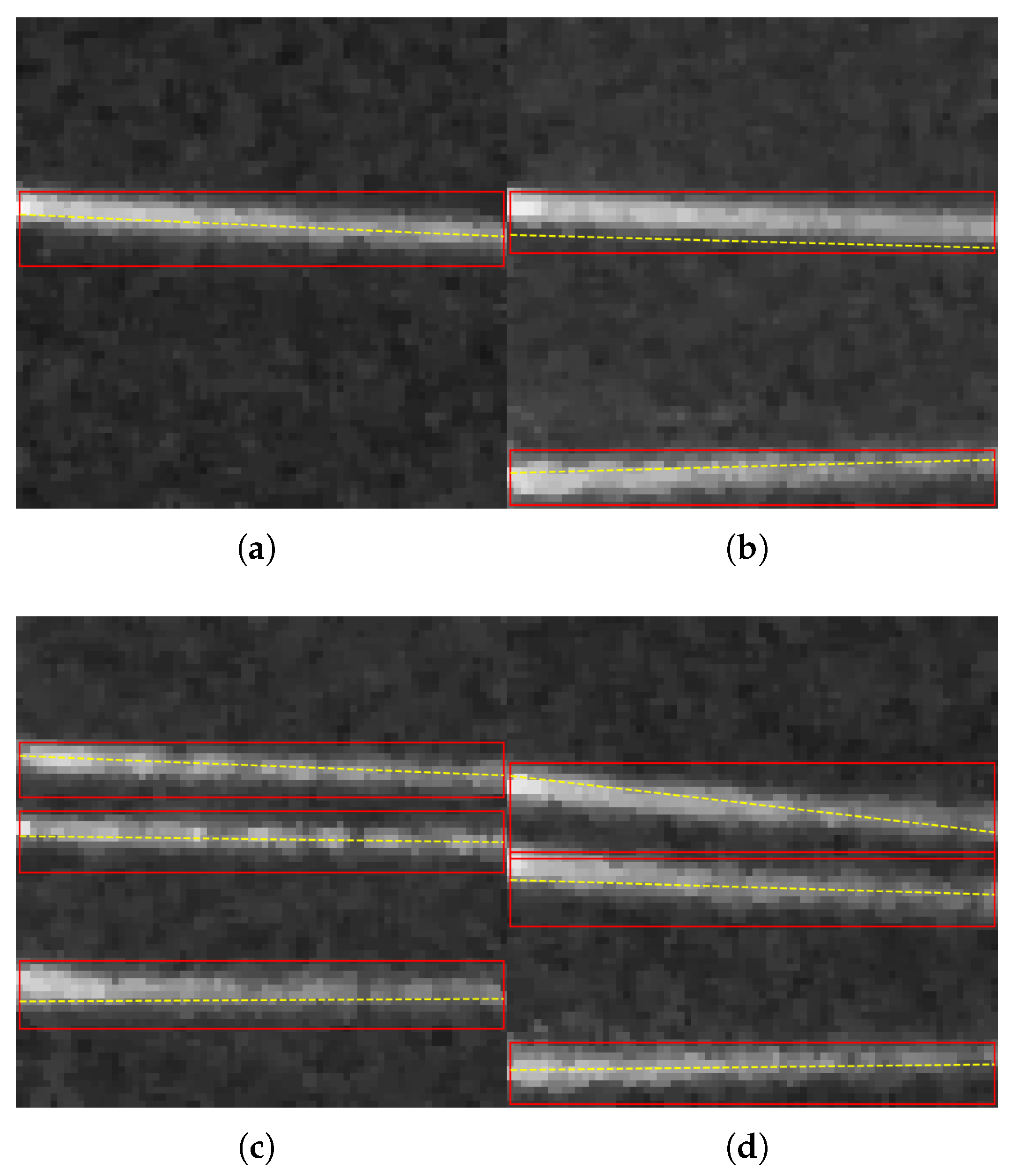
As shown in Figure 6, these frames contain elongated, continuous, high-intensity ridges that are clearly distinguishable from the slowly varying background. In (a), the single track is nearly horizontal and has a strong contrast along most of its length, so the detector produces one stable bounding box and a consistent center line. In (b), two tracks are well separated in the vertical direction, which reduces overlap during NMS and allows both instances to be retained with reliable line estimates. In (c), three parallel tracks remain distinct and approximately uniform in width, which matches the training prior and leads to consistent geometry estimation across multiple instances. In (d), the upper track has a moderate tilt but remains long and continuous. In contrast, the three lower tracks are nearly parallel and non-overlapping, so the detector can localize each track and recover its orientations.
Figure 6.
Representative successful predictions on real beam test data. The red boxes indicate detected track regions and the yellow dashed lines show the estimated track center lines. (a) single-track example; (b) two-track example; (c) three-track example; (d) four-track example.
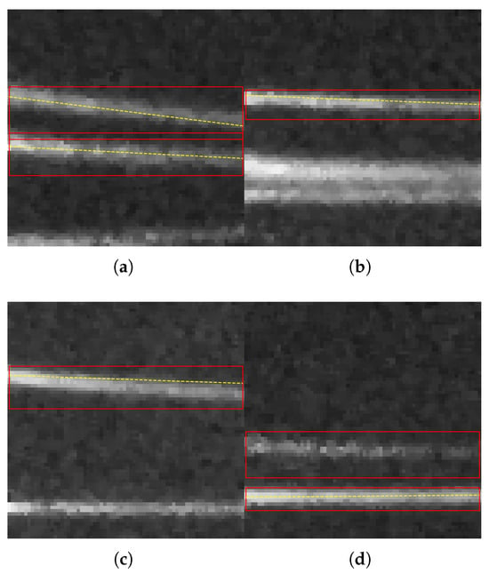
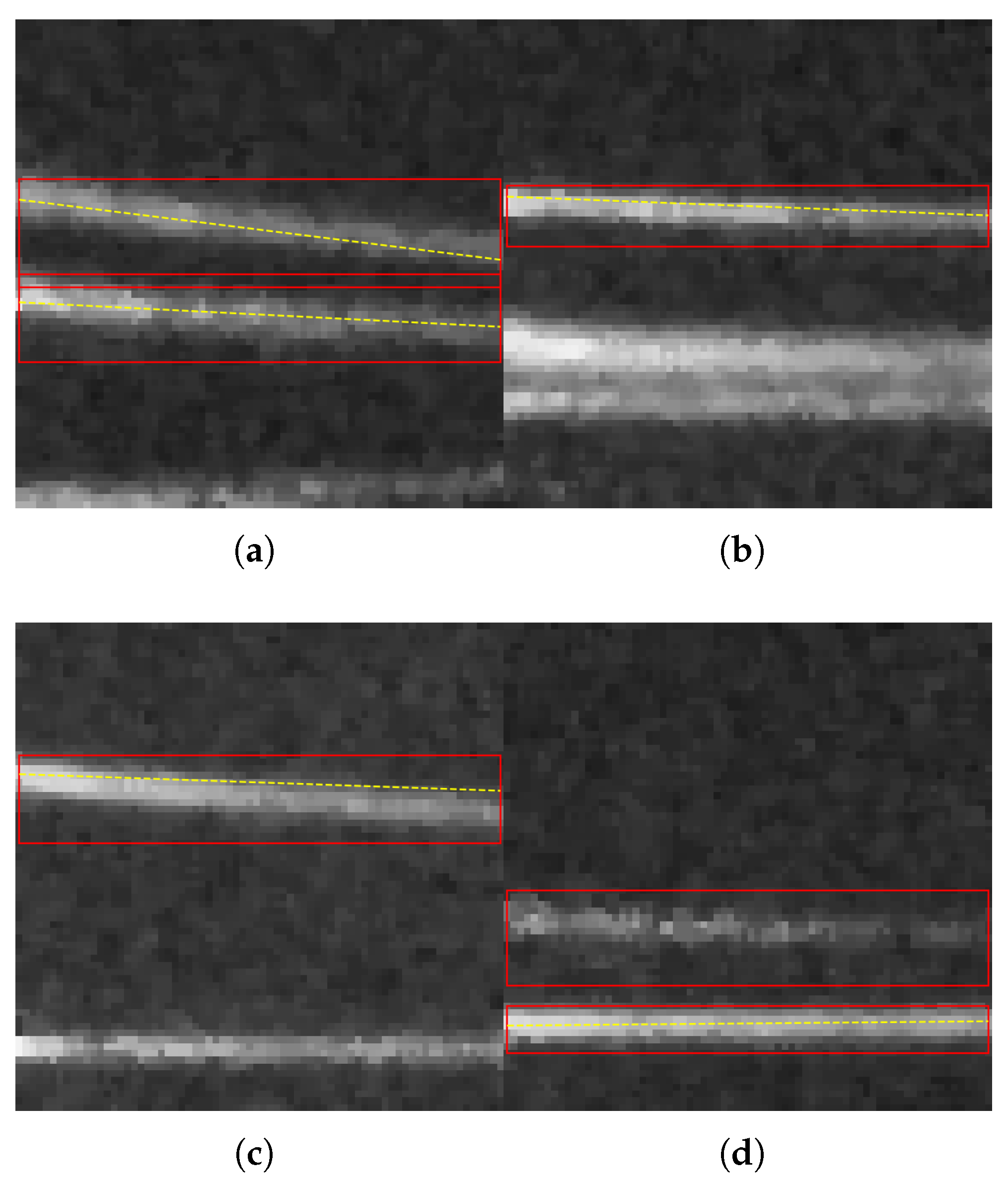
The failure cases in Figure 7 mainly originate from track appearance deviations that are not well covered by the nominal examples. In (a), the projected track lies close to the image boundary and becomes partially truncated, so the visible segment is incomplete and the detector cannot recover a consistent instance. In (b), two tracks overlap and appear as a single merged bright band whose effective width exceeds the normal range, which tends to confuse the detector and leads to missed or incorrect predictions. In (c), the track is fragile, with weak spatial support, making it difficult to separate from background fluctuations and leading to a missed detection. In (d), the track intensity is intermittent, breaking into short fragments, violating the ridge continuity assumption, and leading to a failed localization.
Figure 7.
Representative failure cases on real beam test data. The red boxes indicate detected track regions, and yellow dashed lines indicate the estimated track center lines. (a) truncated track near the image boundary; (b) overlapping tracks merged into a wide band; (c) weak track with low contrast; (d) intermittent track with fragmented intensity.
These results highlight the model’s limitations, indicating that it performs well under conditions with well-defined, uninterrupted tracks but may struggle in scenarios with partial visibility, overlapping tracks, low intensity, or fragmented tracks.
The quantitative results are summarized in Table 5, which lists the detection metrics together with the position resolution. For the current beam test set, the detector maintains a precision of 0.9156 and a recall of 0.9626, and the position resolution remains at the level of a small fraction of a pixel. This indicates that the model retains most of its synthetic domain performance when applied to real beam data.
Table 5.
Detection and line parameter regression performance on real beam test data.
4. Deployment on the U200 Accelerator
4.1. Hardware Platform and Vitis AI Deployment Flow
To demonstrate that the proposed detector can be used for online SEE monitoring, the model is deployed on a data center accelerator card. The experiments in this chapter are carried out on a server equipped with an Alveo U200 card from Xilinx, San Jose, CA, USA. This card contains a large amount of programmable logic, dedicated digital signal processing slices and UltraRAM blocks for on chip buffering. The card is attached to the host through a PCI Express interface, and it is managed by the Xilinx runtime and the Vitis AI software stack.
The deployment follows the standard Vitis AI flow for convolutional neural networks. First, the network is trained in PyTorch v2.9.1 in floating point precision as described in the previous chapters. The trained weights are then exported to an intermediate representation that is compatible with the Vitis AI quantizer. In the next step, the model is quantized to INT8 format using a calibration set drawn from the synthetic validation data. Activations and weights are both quantized, while the overall network topology remains unchanged. The quantized model is then compiled by the Vitis AI compiler to generate a device specific executable in the xmodel format that targets a pre-configured deep learning processing unit on the U200 card.
At run time, the host program loads the compiled xmodel through the Vitis AI runtime and dispatches inference jobs to the U200. Each projection frame is replicated to three channels, resized to , and transferred to the accelerator. The Deep Processing Unit (DPU) operates at 300 MHz and performs the convolutional computation in INT8, returning the raw head outputs that are subsequently parsed to obtain the bounding boxes and line parameters .
4.2. FPGA Resource Utilization and Performance on Beam Test Data
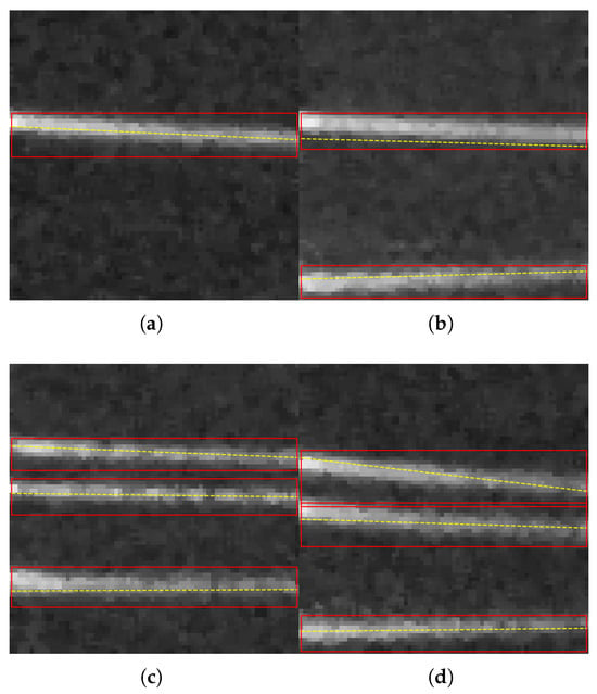
The deployment on the U200 uses only a moderate fraction of the available logic, memory and arithmetic resources. Table 6 summarizes the resource utilization reported by the implementation tools. The design occupies about twelve percent of the look-up tables and fourteen percent of the flip-flop registers, while roughly one third of the digital signal processing slices and UltraRAM blocks are used. This leaves substantial headroom for possible extensions such as multiple detector instances or more complex post-processing stages. Several representative frames processed on the U200 card are shown in Figure 8.
Table 6.
FPGA resource utilization of the deployed detector on the U200 card.
Figure 8.
Example predictions on real beam test data processed by the deployed detector on the U200 card. The red boxes indicate detected track regions and the yellow dashed lines show the estimated track center lines. (a) single-track example; (b) two-track example; (c) three-track example 1; (d) three-track example 2.
We evaluated the runtime performance of the deployed detector using projection frames of size . The hardware latency, defined as the time spent on the U200 accelerator for DPU inference, is approximately 3.1 ms. To characterize the system in a practical online scenario, we also measured end-to-end latency, including the host-side latency. The measured end-to-end latency is approximately 3.4 ms per frame. Because the input payload is compact and the output is sparse, the CPU-side post-processing remains computationally lightweight.
To validate the detection and measurement fidelity of the deployed model, the U200 implementation was applied to the heavy-ion beam test dataset described in the previous section. Table 7 summarizes the quantitative results. The deployed detector achieves a precision of 0.9021 and a recall of 0.9474. In terms of geometric accuracy, the MAE for the line parameters is 0.6824° for the angle and 0.6941 pixels for the intercept, corresponding to a position resolution of 62.84 μm. These results indicate that the accelerator deployment maintains practical measurement fidelity while satisfying the requirement for real-time monitoring.
Table 7.
Detection and line parameter performance of the deployed detector on U200 for real beam test data.
In a practical online SEE monitoring system, the proposed detector can be integrated as a front-end module in a streaming pipeline. Projection frames acquired from the Topmetal sensor are buffered on the host and continuously forwarded to the U200 over Peripheral Component Interconnect Express. The accelerator performs inference and returns the compact detection results, including bounding boxes and the regressed line parameters , to the host. These track parameters are then directly consumed by downstream modules for event building, rate and quality monitoring, real-time visualization, and logging.
Table 8 shows that the FPGA deployment on Alveo U200 provides substantially higher throughput than the representative embedded accelerators reported in the literature. The embedded platforms achieve 56.0–83.3 Frames Per Second (FPS) under low-power budgets, whereas the U200 sustains 322.6 FPS with a YOLOv5n-based detector. This throughput margin is important for online SEE monitoring, where frame bursts and increased track multiplicity can occur and where additional processing may be enabled without compromising real-time operation. System-level requirements further support the choice of an FPGA. The U200 implementation follows a streaming dataflow with fixed timing, which facilitates deterministic latency budgeting and robust integration with the readout chain. In this setting, throughput headroom and timing determinism are prioritized over minimum power, making the U200-based FPGA solution more suitable than embedded graphics processing unit alternatives for the targeted beam-test deployment.
Table 8.
Quantitative comparison of representative edge accelerators.
5. Conclusions
This work presents a lightweight YOLOv5n-based detector for online localization of heavy-ion track projections in Topmetal pixel sensor images. The proposed method formulates track localization as an object detection problem and performs a single forward pass to predict both bounding boxes and the physically meaningful line parameters , thereby avoiding a separate geometric fitting stage and improving robustness to noise and partial tracks. On a synthetic dataset, the detector achieves a precision/recall of 0.9626/0.9493, with an MAE of 0.3930° in angle and 0.4842 pixels in intercept. On krypton beam measurements, it reaches a precision/recall of 0.9156/0.9626 and delivers a position resolution of 52.05 μm. We further demonstrate FPGA deployment on an Alveo U200, achieving an average accelerator latency of 3.1 ms per frame while maintaining measurement quality. Overall, the proposed approach enables accurate and low-latency track localization suitable for integration into continuous, online SEE monitoring pipelines.
Author Contributions
Conceptualization, Z.M. and Z.S.; methodology, W.T.; software, Z.S. and W.T.; validation, Z.S., W.T. and J.L.; formal analysis, H.W. (Hongxia Wang) and H.W. (Haoran Wu); investigation, Z.S.; resources, W.D. and G.H.; data curation, Y.G., J.L. and K.J.; writing—original draft preparation, Z.S. and W.T.; writing—review and editing, W.D. and J.L.; visualization, Z.S. and W.T.; supervision, Z.M. and G.H.; project administration, Z.S. and W.T.; funding acquisition, W.D. and G.H. All authors have read and agreed to the published version of the manuscript.
Funding
This research was funded by the National Natural Science Foundation of China under Grant No. 12205224, and the Key Research and Development Special Project of Hubei Provincial Technology Innovation Program under Grant No. 2023BCB086.
Institutional Review Board Statement
Not applicable.
Informed Consent Statement
Not applicable.
Data Availability Statement
The data that support the findings of this study are available from the corresponding author upon reasonable request.
Conflicts of Interest
The authors declare no conflicts of interest.
Abbreviations
The following abbreviations are used in this manuscript:
| SEE | Single Event Effect |
| FPGA | Field-Programmable Gate Array |
| RANSAC | Random Sample Consensus |
| YOLO | You Only Look Once |
| NMS | Non-Maximum Suppression |
| CIoU | Complete Intersection over Union |
| MAE | Mean Absolute Error |
| ROI | Region of Interest |
| SNR | Signal-to-Noise Ratio |
| mAP | mean Average Precision |
| HIRFL | Heavy Ion Research Facility in Lanzhou |
| DPU | Deep Processing Unit |
| FPS | Frames Per Second |
References
- Gaillard, R. Single Event Effects: Mechanisms and Classification. In Soft Errors in Modern Electronic Systems; Springer: Berlin/Heidelberg, Germany, 2011; pp. 27–54. [Google Scholar] [CrossRef] [Scilit]
- Normand, E. Single-Event Effects in Avionics. IEEE Trans. Nucl. Sci. 1996, 43, 461–474. [Google Scholar] [CrossRef] [Scilit]
- Petersen, E. Single Event Effects in Aerospace; Wiley-IEEE Press: Piscataway, NJ, USA, 2011. [Google Scholar]
- Sexton, F.W. Destructive Single-Event Effects in Semiconductor Devices and ICs. IEEE Trans. Nucl. Sci. 2003, 50, 603–621. [Google Scholar] [CrossRef] [Scilit]
- Chen, Q.; Guo, G.; Sui, L.; Liu, J.; Zhang, Y.; Zhang, F.; Yin, Q.; Han, J.; Zhang, Z.; Sun, H. Accelerator Simulation Test Technology and Its Application for Single Event Effect Evaluation in Space. Nucl. Tech. 2023, 46, 080008. [Google Scholar] [CrossRef]
- Buchner, S.P.; Miller, F.; Pouget, V.; McMorrow, D.P. Pulsed-Laser Testing for Single-Event Effects Investigations. IEEE Trans. Nucl. Sci. 2013, 60, 1852–1875. [Google Scholar] [CrossRef] [Scilit]
- Guo, J.; Du, G.; Bi, J.; Liu, W.; Wu, R.; Chen, H.; Wei, J.; Li, Y.; Sheng, L.; Liu, X.; et al. Development of Single-Event-Effects Analysis System at the IMP Microbeam Facility. Nucl. Instrum. Methods Phys. Res. Sect. B 2017, 404, 250–253. [Google Scholar] [CrossRef] [Scilit]
- He, Y.; Zhao, J.; Shu, W.; Chong, K.S.; Chang, J. Radiation-Induced Failures for Integrated Circuits in Space and Design Philosophy. In Proceedings of the 2022 IEEE International Symposium on the Physical and Failure Analysis of Integrated Circuits (IPFA), Singapore, 18–21 July 2022; IEEE: Piscataway, NJ, USA, 2022; pp. 1–4. [Google Scholar] [CrossRef] [Scilit]
- Li, Z.; Fan, Y.; Wang, Z.; Liu, J.; Sun, X.; Zhao, C.; Pei, H.; Wang, D.; Huang, G.; Zhang, D.; et al. A New Method for Directly Locating Single-Event Latchups Using Silicon Pixel Sensors in a Gas Detector. Nucl. Instrum. Methods Phys. Res. Sect. A 2020, 962, 163697. [Google Scholar] [CrossRef] [Scilit]
- Liu, J.; Gao, C.; Wang, H.; Wang, Z.; You, B.; Sun, X.; Chen, K.; Yang, P.; Guo, D.; Xiao, L.; et al. Design and Preliminary Characterization of a Novel Silicon Charge Sensor for the Gaseous Beam Monitor at the CSR External-Target Experiment. Nucl. Instrum. Methods Phys. Res. Sect. A 2023, 1047, 167786. [Google Scholar] [CrossRef] [Scilit]
- Gao, C.; Huang, G.; Sun, X. Topmetal-II: A Direct Charge Sensor for High Energy Physics and Imaging Applications. J. Instrum. 2016, 11, C01053. [Google Scholar] [CrossRef] [Scilit]
- Krider, J. Residual Gas Beam Profile Monitor. Nucl. Instrum. Methods Phys. Res. Sect. A 1989, 278, 660–663. [Google Scholar] [CrossRef] [Scilit]
- El-Sisi, A.B. Wire Scanner Beam Profile Measurement for ESRF. In Proceedings of the DIPAC 2003 (6th European Workshop on Beam Diagnostics and Instrumentation for Particle Accelerators), Mainz, Germany, 5–7 May 2003. [Google Scholar]
- Stelzer, H. Multiwire Chambers with a Two-Stage Gas Amplification. Nucl. Instrum. Methods Phys. Res. Sect. A 1991, 310, 103–106. [Google Scholar] [CrossRef] [Scilit]
- Yang, H.; Zhang, H.; Gao, C.; Wang, H.; Sun, X.; Liu, J.; Wang, S.; Li, X.; Ren, W.; Zhou, W.; et al. Hi’Beam-S: A Monolithic Silicon Pixel Sensor-Based Prototype Particle Tracking System for HIAF. IEEE Trans. Nucl. Sci. 2021, 68, 2794–2800. [Google Scholar] [CrossRef] [Scilit]
- Illingworth, J.; Kittler, J. A survey of the Hough transform. Comput. Vis. Graph. Image Process. 1988, 44, 87–116. [Google Scholar] [CrossRef] [Scilit]
- Fischler, M.A.; Bolles, R.C. Random Sample Consensus: A Paradigm for Model Fitting with Applications to Image Analysis and Automated Cartography. Commun. ACM 1981, 24, 381–395. [Google Scholar] [CrossRef] [Scilit]
- Baranov, D.; Mitsyn, S.; Goncharov, P.; Ososkov, G. The Particle Track Reconstruction based on deep Neural Networks. arXiv 2018, arXiv:1812.03859. [Google Scholar] [CrossRef] [Scilit]
- Zdybał, M.; Asenov, P.; Driutti, A.; Goncerz, M.; Hess, E.; Kucharczyk, M.; Mizera, D.; Wolter, M. Machine learning based event reconstruction for the MUonE experiment. EPJ Web Conf. 2025, 337, 01255. [Google Scholar] [CrossRef] [Scilit]
- Brooke, J.; Clement, E.; Glowacki, M.; Paramesvaran, S.; Segal, J. FPGA implementation of a CNN-based topological trigger for HL-LHC. Comput. Softw. Big Sci. 2025, 9, 18. [Google Scholar] [CrossRef] [Scilit] [PubMed]
- Redmon, J.; Divvala, S.; Girshick, R.; Farhadi, A. You Only Look Once: Unified, Real-Time Object Detection. In Proceedings of the IEEE Conference on Computer Vision and Pattern Recognition (CVPR), Las Vegas, NV, USA, 27–30 June 2016; IEEE: Piscataway, NJ, USA, 2016; pp. 779–788. [Google Scholar] [CrossRef] [Scilit]
- Liu, Y.; He, G.; Wang, Z.; Li, W.; Huang, H. NRT-YOLO: Improved YOLOv5 Based on Nested Residual Transformer for Tiny Remote Sensing Object Detection. Sensors 2022, 22, 4953. [Google Scholar] [CrossRef] [Scilit]
- Tian, J.H.; Feng, X.F.; Li, F.; Xian, Q.-L.; Jia, Z.-H.; Liu, J.-L. An Improved YOLOv5n Algorithm for Detecting Surface Defects in Industrial Components. Sci. Rep. 2025, 15, 9756. [Google Scholar] [CrossRef] [Scilit]
- Duda, R.O.; Hart, P.E. Use of the Hough transformation to detect lines and curves in pictures. Commun. ACM 1972, 15, 11–15. [Google Scholar] [CrossRef] [Scilit]
- Gabrielli, A.; Alfonsi, F.; Del Corso, F. Hough Transform Proposal and Simulations for Particle Track Recognition for LHC Phase-II Upgrade. Sensors 2022, 22, 1768. [Google Scholar] [CrossRef] [Scilit]
- Ayyad, Y.; Mittig, W.; Bazin, D.; Beceiro-Novo, S.; Cortesi, M. Novel particle tracking algorithm based on the random sample consensus model for the active target time projection chamber (AT-TPC). Nucl. Instrum. Methods Phys. Res. Sect. A 2018, 880, 166–173. [Google Scholar] [CrossRef] [Scilit]
- Jocher, G.; Stoken, A.; Chaurasia, A.; Borovec, J.; Kwon, Y.; Michael, K.; Changyu, L.; Fang, J.; Skalski, P.; Hogan, A.; et al. ultralytics/yolov5: V6. 0-YOLOv5n’Nano’models, Roboflow integration, TensorFlow export, OpenCV DNN support. Zenodo 2021. [Google Scholar] [CrossRef]
- Bie, M.; Liu, Y.; Li, G.; Hong, J.; Li, J. Real-time vehicle detection algorithm based on a lightweight You-Only-Look-Once (YOLOv5n-L) approach. Expert Syst. Appl. 2023, 213, 119108. [Google Scholar] [CrossRef] [Scilit]
- Wang, C.; Wang, C.; Wang, L.; Wang, J.; Liao, J.; Li, Y.; Lan, Y. A lightweight cherry tomato maturity real-time detection algorithm based on improved YOLOV5n. Agronomy 2023, 13, 2106. [Google Scholar] [CrossRef] [Scilit]
- Qiao, W.; Guo, H.; Huang, E.; Su, X.; Li, W.; Chen, H. Real-Time Detection of Slug Flow in Subsea Pipelines by Embedding a Yolo Object Detection Algorithm into Jetson Nano. J. Mar. Sci. Eng. 2023, 11, 1658. [Google Scholar] [CrossRef] [Scilit]
- Shin, D.J.; Kim, J.J. A Deep Learning Framework Performance Evaluation to Use YOLO in Nvidia Jetson Platform. Appl. Sci. 2022, 12, 3734. [Google Scholar] [CrossRef] [Scilit]
- Kang, P.; Somtham, A. An Evaluation of Modern Accelerator-Based Edge Devices for Object Detection Applications. Mathematics 2022, 10, 4299. [Google Scholar] [CrossRef] [Scilit]

Disclaimer/Publisher’s Note: The statements, opinions and data contained in all publications are solely those of the individual author(s) and contributor(s) and not of MDPI and/or the editor(s). MDPI and/or the editor(s) disclaim responsibility for any injury to people or property resulting from any ideas, methods, instructions or products referred to in the content. |
© 2026 by the authors. Licensee MDPI, Basel, Switzerland. This article is an open access article distributed under the terms and conditions of the Creative Commons Attribution (CC BY) license.