Multi-Time-Scale Coordinated Optimization Scheduling Strategy for Wind–Solar–Hydrogen–Ammonia Systems

Abstract

To address the inherent mismatch between the fluctuating power output of renewable energy and the continuous production requirements of ammonia in off-grid wind–solar–hydrogen–ammonia systems, this paper proposes a “day-ahead–intraday–real-time” multi-time-scale coordinated optimization scheduling strategy. In the day-ahead layer, Wasserstein Distributionally Robust Optimization (WDRO) is employed to determine a conservative and stable baseline plan for ammonia load under high uncertainty of wind and solar output. The intraday layer utilizes Model Predictive Control (MPC) with a 2-h prediction horizon and 15-min rolling steps to correct short-term forecast deviations. The real-time layer achieves minute-level power balancing through priority dispatch and deadband control. Furthermore, hydrogen storage tanks serve as a material buffer between hydrogen production and ammonia synthesis, with their state variables transmitting across layers to achieve flexible multi-time-scale coupling. Simulation results demonstrate that, although this strategy slightly reduces the theoretical maximum ammonia yield, it completely avoids load-shedding risks. Compared with the deterministic scheduling (Scheme 1), which suffers a net loss due to severe penalty costs, the proposed strategy achieves a positive daily profit of CNY 277,700, representing an absolute increase of CNY 429,300. Furthermore, it provides an additional daily profit of CNY 65,800 compared to the stochastic optimization approach (Scheme 2), demonstrating superior economic robustness in off-grid environments.

1. Introduction

With the deep implementation of “Dual Carbon” strategies (carbon peaking and car-bon neutrality), wind–solar–hydrogen–ammonia technology has become a research hotspot in the energy and chemical sectors due to its dual advantages of realizing on-site consumption of renewable energy and producing green chemical raw materials [1,2,3]. However, in the off-grid operation mode, there exists a significant spatio-temporal mis-match and dynamic incompatibility between the strong stochasticity and high volatility of natural wind and solar resources and the strict requirements of the ammonia synthesis process for feed continuity. Breaking the time-scale barriers of source–load matching un-der the rigid constraints of “intermittent source versus steady load” to achieve efficient synergy and safe, stable operation has become a key bottleneck restricting the large-scale industrialization of this technology [4,5,6].

Existing research on wind–solar–hydrogen–ammonia systems mainly covers two dimensions: capacity planning and operation scheduling. In terms of capacity planning, Ref. [7] constructed a joint capacity–scheduling optimization model for grid-connected/off-grid systems, analyzing the impact of different wind–solar ratios on the life-cycle revenue of the system. Ref. [8] verified the economic feasibility of using ammonia as a carrier for cross-seasonal energy storage. Ref. [9] introduced an adaptive distributionally robust optimization (DRO) method, effectively alleviating the conservativeness of traditional planning methods. These studies have laid a solid foundation for system equipment selection. These studies provide valuable insights into equipment sizing but typically adopt single-layer formulations and implicitly assume that the ammonia synthesis unit can respond flexibly to power fluctuations.

In reality, ammonia synthesis is governed by the thermal dynamics of the catalyst bed, exhibiting strong operational rigidity and thermal inertia. This creates an inherent tension between the multi-timescale variability of renewable generation (from minutes to hours) and the continuous, stable operation required by chemical reactors—a critical challenge for off-grid industrial deployment that remains inadequately addressed.

Regarding operational scheduling, most works focus on single time scales or individual components. For instance, Ref. [10] employed stochastic model predictive control (MPC) for rolling rescheduling in off-grid systems, while Refs. [11,12] explored “multi-steady-state flexible processes” to enhance source–load matching through wide-range load modulation. Nevertheless, these approaches still treat ammonia synthesis as a dispatchable load, overlooking its physical constraints.

Although multi-time-scale frameworks have been established in related domains—such as multi-microgrids [13] and hydro-powered hydrogen production [14,15]—their direct application to off-grid chemical synthesis systems faces three fundamental limitations: (1) Conceptual Mismatch in Safety Boundaries: Most stochastic optimization (SO) or robust optimization (RO) methods treat the ammonia load merely as a flexible electrical demand similar to a battery. They fail to mathematically formulate the rigid safety boundary required by the chemical reaction’s thermal stability. Consequently, these methods cannot theoretically guarantee continuous operation under worst-case probability distributions of wind/solar output. (2) Insufficient mining of the “time decoupling” value of the hydrogen storage link: Hydrogen tanks are often simplified as energy storage units, and their roles as material buffers for low-pass filtering and time-scale decoupling between high-frequency hydrogen production and low-frequency hydrogen consumption have not been fully utilized. (3) Absence of interlayer closed-loop feedback mechanisms: The existing “day-ahead planning–real-time execution” mode lacks effective information interaction between layers. There is a lack of effective state feedback between the robust decision-making of the day-ahead layer and the rolling correction of the intraday layer, making it difficult to achieve the unification of global economic optimality and real-time safety response.

To address the above limitations, this paper proposes a multi-time-scale coordinated optimization scheduling strategy based on the concept of “rigid protection for ammonia synthesis and flexible regulation of electrolyzers” for an off-grid wind–solar–hydrogen–ammonia system with configured capacity. The main contributions are as follows:

(1)

Methodological Advancement: A Distributionally Robust Safety Baseline. Unlike traditional stochastic methods that optimize for expected scenarios, we introduce a Wasserstein Distributionally Robust Optimization (WDRO) framework in the day-ahead layer. By constructing a ‘Wasserstein ambiguity set’ centered on empirical distributions, this method establishes a mathematically proven ‘Safety Baseline’ for the ammonia load. This theoretically ensures that the chemical process remains within its safe operating envelope even under worst-case distribution shifts, effectively resolving the conflict between renewable uncertainty and chemical rigidity.

(2)

Innovation in Control Mechanism: We have introduced a frequency-domain separation (spectral separation) mechanism for source–load matching. By implementing “rigid follow-up” for the ALK (handling steady-state power) at the real-time layer, and “flexible adjustment” for the PEM/battery (handling transient fluctuations), we effectively resolve the physical incompatibility between fluctuation sources and stable loads.

(3)

Architecture Enhancement: We construct a closed-loop feedback system across time scales. By utilizing the Hydrogen Tank Level (SOC_H2) as a coupling state variable, we link the long-term robust planning with short-term real-time response, enhancing the system’s dynamic resilience compared to open-loop strategies.

2. System Model of Wind–Solar–Hydrogen–Ammonia Production

Given that this paper involves many parameters, the explanations of these parameters will be provided in

Table 1. Explanation of Parameters.

Parameters	Description
$P_{\mathrm{ALK},\mathrm{t}}$/$P_{\mathrm{PEM},\mathrm{t}}$	Power of the ALK and PEM electrolysis cells at time period t (Unit: MW)
$\Delta P^{\max }$	Maximum climbing power limit (Unit: MW)
$u_{\mathrm{ALK},\mathrm{t}}$/$u_{\mathrm{PEM},\mathrm{t}}$	0–1 Start-stop status variable
$P_{\mathrm{ALK}}^{\min }$/$P_{\mathrm{ALK}}^{\max }$	The minimum and maximum power of the ALK (Unit: MW)
$P_{\mathrm{PEM}}^{\min }$/$P_{\mathrm{PEM}}^{\max }$	The minimum and maximum power of the PEM (Unit: MW)
$m_{{\mathrm{H}}_2,\mathrm{ALK},\mathrm{t}}$/$m_{{\mathrm{H}}_2,\mathrm{PEM},\mathrm{t}}$	The hydrogen production rate of the ALK and PEM during period t (Unit: kg/h)
${\eta }_{\mathrm{ALK}}$/${\eta }_{\mathrm{PEM}}$	The unit hydrogen production energy consumption of the ALK and PEM electrolysis cells (Unit: MWh/kg)
$P_{\mathrm{ASU},\mathrm{t}}$	The power of the time-sharing nitrogen generation device at time t (Unit: MW)
$P_{\mathrm{ASU}}^{\min }$/$P_{\mathrm{ASU}}^{\max }$	The minimum and maximum values of the power of the air separation nitrogen production unit (Unit: MW)
$m_{{\mathrm{N}}_2,\mathrm{ASU},\mathrm{t}}$	The nitrogen production rate of the time-sharing nitrogen generation device at time t (Unit: kg/h)
${\eta }_{\mathrm{ASU}}$	Energy consumption per unit production of nitrogen in the air separation unit (Unit: MW)
$P_{{\mathrm{NH}}_3,\mathrm{t}}$	Power of the ammonia synthesis plant at time t (Unit: MW)
$P_{{\mathrm{NH}}_3}^{\min }$/$P_{{\mathrm{NH}}_3}^{\max }$	Minimum and maximum power of the ammonia synthesis plant (Unit: MW)
$\Delta P_{{\mathrm{NH}}_3}^{\max }$	Single-step maximum adjustment amount (Derived from ≤1%/min ramp rate limit; 15% for intraday, 5% for real-time) (Unit: MW)
$o$	Minimum load factor
$P_{{\mathrm{NH}}_3}^{\mathrm{rated}}$	The rated power of the ammonia synthesis plant (70 MW)
$m_{{\mathrm{H}}_2,\mathrm{out},\mathrm{t}}$/$m_{{\mathrm{N}}_2,\mathrm{out},\mathrm{t}}$	The hydrogen and nitrogen consumption rates of the ammonia synthesis plant (Unit: kg/h)
${\eta }_{{\mathrm{NH}}_3}$	Energy consumption per unit output of ammonia synthesis (Unit: MWh/kg)
${\alpha }_{{\mathrm{H}}_2}$/${\alpha }_{{\mathrm{N}}_2}$	The hydrogen and nitrogen consumption coefficients for unit synthesis ammonia production
$P_{\mathrm{bat},\mathrm{t}}$	Battery power at time period t, positive for charging and negative for discharging (Unit: MW)
$P_{\mathrm{bat}}^{\max }$	Maximum charging and discharging power (Unit: MW)
$SO{C}^{\min }$/$SO{C}^{\max }$	Minimum and maximum values of charge state
$\Delta t$	Time step
$E_{\mathrm{bat}}$	Battery rated capacity (Unit: MWh)
$SO{C}_{{\mathrm{H}}_2,\mathrm{t}}$	Normalized hydrogen storage volume of the storage tank at time t
$SO{C}_{{\mathrm{H}}_2}^{\min }$/$SO{C}_{{\mathrm{H}}_2}^{\max }$	Minimum and maximum storage capacity of the hydrogen storage tank
$m_{{\mathrm{H}}_2,\mathrm{in},\mathrm{t}}$	The total hydrogen production rate of the electrolyzer at time t (Unit: MWh/kg)
$V_{{\mathrm{H}}_2}^{\max }$	The maximum volume of the hydrogen storage tank (Unit: kg)
$SO{C}_{{\mathrm{N}}_2}$	Normalized nitrogen storage volume of the storage tank at time t
$SO{C}_{{\mathrm{N}}_2}^{\min }$/$SO{C}_{{\mathrm{N}}_2}^{\max }$	Minimum and maximum values of nitrogen storage tank capacity
$m_{{\mathrm{N}}_2,\mathrm{in},\mathrm{t}}$	Nitrogen production rate of the space division device at time t (Unit: MWh/kg)
$V_{{\mathrm{N}}_2}^{\max }$	The maximum capacity of the nitrogen storage tank (Unit: kg)
$P_{\mathrm{ren},t}$	Total power output of wind and solar energy at time t (Unit: MW)
$P_{\mathrm{curt},t}$	The wind and solar power that was discarded due to the system’s inability to accommodate it (Unit: MW)
$P_{\mathrm{shed},\mathrm{t}}$	The power load of synthetic ammonia removed in emergency situations (Unit: MW)
$P_{{\mathrm{NH}}_3}^{\mathrm{base}}$	Power benchmark of the ammonia synthesis plant (Unit: MW)
$\xi$	The uncertain parameter is the sequence of power output from the wind and solar sources.
$\kappa$	The feasible region of the decision variables
${\widehat{P}}_{\mathrm{N}}$	The empirical distribution constructed based on N historical scenarios
$B_{\vartheta }({\widehat{P}}_{\mathrm{N}})$	Centered on the empirical distribution, a Wasserstein ball with a radius of $\vartheta$
$L(P_{{\mathrm{NH}}_3}^{\mathrm{base}},\xi )$	Loss function under given decisions and scenarios
$ℝ(\delta )$	The set of all probability distributions over the parameter space $\delta$
$W_{\mathrm{p}}(P,{\widehat{P}}_{\mathrm{N}})$	The p-Wasserstein distance between the distribution $P$ and the empirical distribution ${\widehat{P}}_{\mathrm{N}}$
${\widehat{P}}_{\mathrm{ren},\mathrm{t}}$	The current forecasted wind power value (Unit: MW)
${\epsilon }^{(\mathrm{s})}(\mathrm{t})$	The relative predicted error of the s-th scene during the $\mathrm{t}$ period
$\mathbb{N}(0,1)$	Standard normal distribution, depicting the random fluctuations of prediction errors
$u(0,1)$	Uniformly distributed within [0, 1], depicting the systematic shift in the direction of prediction bias
${\sigma }_{\mathrm{base}}$	Control the intensity of random fluctuations, with a value of 0.2
${\sigma }_{\mathrm{bias}}$	The control system has an offset intensity of 0.1.
$L_{SOC}^{(\mathrm{s})}$	Battery SOC out-of-limit penalty
${\gamma }_{\mathrm{low}}$/${\gamma }_{\mathrm{high}}$	Lower limit over-limit penalty coefficient and upper limit lower limit over-limit penalty coefficient
$L_{SO{C}_{{\mathrm{H}}_2}}^{(\mathrm{s})}$	Terminal constraint penalty for hydrogen storage tanks
${\gamma }_{SO{C}_{{\mathrm{H}}_2}}$	Hydrogen storage tank over-limit penalty coefficient
$SO{C}_{{\mathrm{H}}_2,24}$	Normalized hydrogen storage tank volume at the end of the 24th period in Scenario s
$L(P_{{\mathrm{NH}}_3}^{\mathrm{base}},{\xi }^{(\mathrm{s})})$	Comprehensive loss function
$C_{\mathrm{rev}}$	Ammonia production yield coefficient
$\lambda$	Robustness coefficient, value is 10
$N_{\mathrm{s}}$	Total number of scenes, with a value of 50
$L\left(\mathrm{i}\right)$	The value of the i-th (from the largest to the smallest) loss in all scenarios
$N_p$	Predictive time domain, value is 8
$J_{\mathrm{ALK},\mathrm{k}}$	Power smoothing cost of electrolytic cells
$J_{{\mathrm{NH}}_3,\mathrm{k}}^{\mathrm{track}}$	Tracking costs for the ammonia synthesis project
$P_{{\mathrm{NH}}_3,\mathrm{k}}^{\mathrm{DA}}$	The reference values issued recently
$J_{{\mathrm{NH}}_3,\mathrm{k}}^{\mathrm{smooth}}$	Power smoothing cost for ammonia synthesis
$J_{SOH,\mathrm{k}}^{\mathrm{bound}}$	Cost of boundary penalties for hydrogen storage tanks
${\omega }_{SOH}^{\mathrm{low}}$/${\omega }_{SOH}^{\mathrm{high}}$	Lower limit weight and upper limit weight
$J_{\mathrm{terminal}}$	Terminal state constraints
$SO{C}_{\mathrm{t}+N_{\mathrm{p}}}$	Predict the state of charge of the battery at the end of the process
$SO{C}_{\mathrm{ref}}$	The expected value that the battery should reach at the end of the prediction, 0.5
$SO{C}_{{\mathrm{H}}_2}^{\mathrm{t}+N_p}$	Predict the normalized storage volume of the end-of-pipe hydrogen storage tank
$SO{C}_{{\mathrm{H}}_2}^{\mathrm{ref}}$	The expected state of the hydrogen storage tank at the end of the prediction, 0.5
$V{I}_{\mathrm{t}}$	The fluctuation index at time t
$\rho (\cdot )$	Standard deviation operator
$\mu (\cdot )$	Mean operator
$P_{(\mathrm{t}-\mathsf{\Delta }\mathrm{w}:\mathrm{t})}$	The sequence of power output of the wind and solar energy within the sliding window from time $\mathrm{t}-\Delta w$ to time t
$\Delta w$	Sliding window width, 6
$\phi$	Prevent the introduction of small constants caused by division by zero
${\theta }_{\mathrm{t}}$	The dead zone threshold at time t
${\theta }_0$	Base dead zone coefficient,0.02
$l_{VI}$	Amplification coefficient of fluctuation, 8
$P_{{\mathrm{NH}}_3,\mathrm{t}}^{\mathrm{ID}}$	The power instruction for ammonia synthesis issued by the inner layer (Unit: MW)
$\Delta P$	Power deviation (Unit: MW)
$P_{\mathrm{ALK},\mathrm{t}}^{\mathrm{ref}}$	Expected power reference value of ALK (Unit: MW)
${\alpha }_{DB}$	Dead zone control weight
$1-{\alpha }_{DB}$	Daily plan following the weighting scheme
$P_{\mathrm{bat}}^{\mathrm{dmax}}$	The maximum discharge power allowed by the battery at the present moment (Unit: MW)
$\Delta P_{\mathrm{net},\mathrm{t}}$	Power imbalance of the system at time t (Unit: MW)
$P_{\mathrm{ren},\mathrm{t}}^{\mathrm{pred}}$	Short-term prediction of renewable energy output (Unit: MW)
$P_{\mathrm{start}}$	Pem startup threshold (Unit: MW)
$P_{\mathrm{bat},\mathrm{t}}^{\mathrm{ID}}$	The benchmark charging and discharging power determined through continuous optimization within the day (Unit: MW)
$\Delta P_{\mathrm{bat},\mathrm{t}}^{\mathrm{adj}}$	Real-time power regulation (Unit: MW)
$P_{\mathrm{bat}}^{\mathrm{cmax}}$/$P_{\mathrm{bat}}^{\mathrm{dmax}}$	Consider the maximum charging/discharging power under the current SOC constraints (Unit: MW)
${\beta }_{\mathrm{on}}^{\mathrm{base}}$	Base startup threshold, 0.1
${\beta }_{\mathrm{on}}^{\mathrm{adj}}$	Adjustment coefficient, 0.05

.

2.1. Overall System Architecture

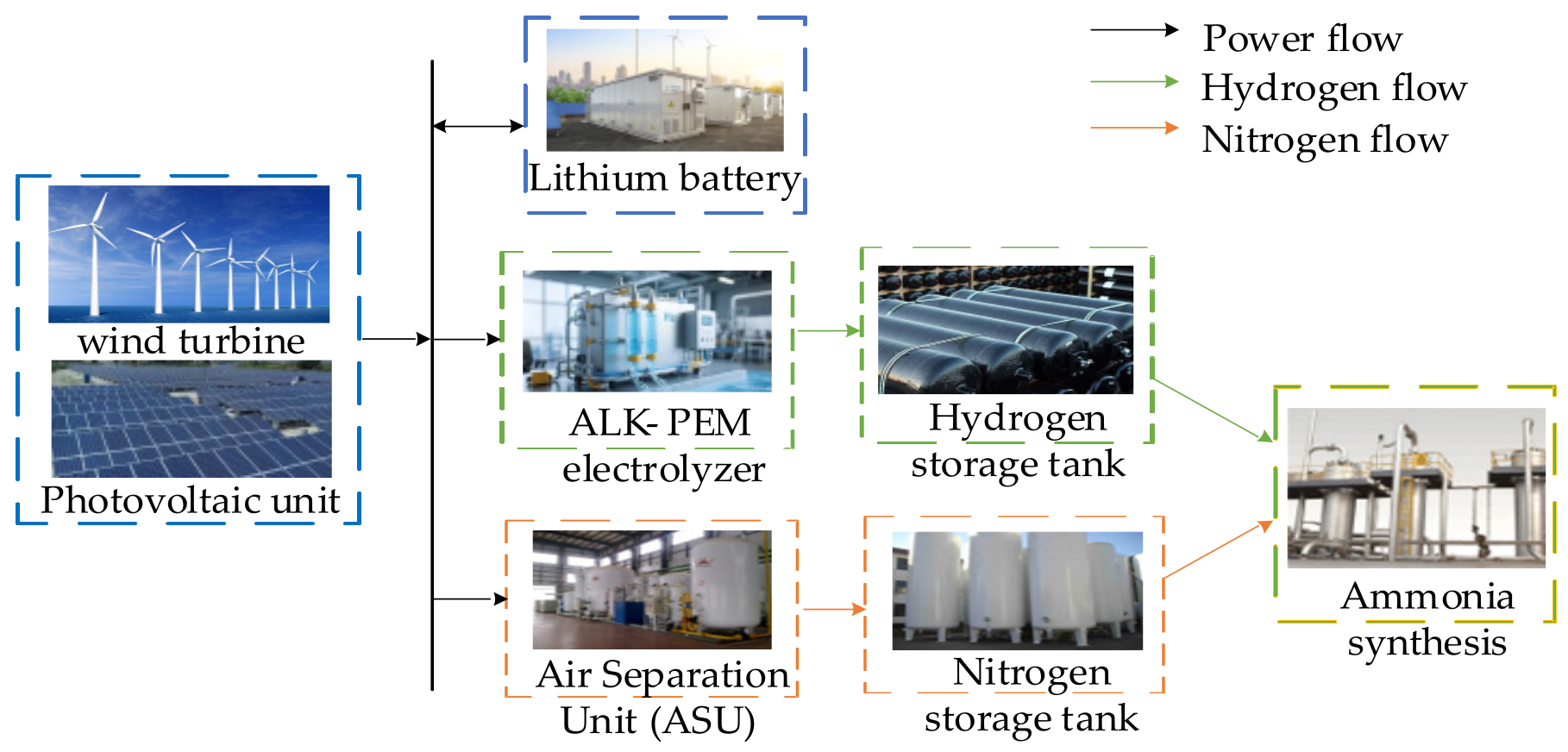
The off-grid wind–solar–hydrogen–ammonia system investigated in this study comprises a wind–solar power generation unit, an electrolytic hydrogen production unit, an air separation unit (ASU), an energy storage unit (including lithium-ion batteries and hydrogen/nitrogen storage tanks), and an ammonia synthesis unit, as illustrated in Figure 1.

In this system, the electrolytic hydrogen production unit adopts a hybrid configuration of the ALK and the PEM. The ALK is utilized to undertake baseload hydrogen production tasks due to its advantages of large capacity and low cost, while the PEM leverages its fast dynamic response characteristics to smooth high-frequency power fluctuations. The hydrogen and nitrogen storage tanks serve as critical material buffer nodes connecting upstream gas generation with downstream chemical processes, thereby achieving time-scale decoupling of the electricity–gas–chemical process. Although the ASU is also an electrical load, given that the energy consumption for nitrogen production is significantly lower than that for hydrogen production (accounting for approximately 3% of the total system energy consumption) and the system is equipped with nitrogen storage tanks of a certain capacity, this paper models it as a rigid auxiliary load that follows the production rhythm of the ammonia synthesis unit.

2.2. Mathematical Models of Each Unit

2.2.1. ALK-PEM Electrolyzer Unit Model

The operation of electrolyzers is constrained by ramp rates and power output boundaries. Considering safety hazards such as gas purity degradation, energy efficiency attenuation, and diaphragm gas crossover under low-load conditions (particularly for ALK electrolyzers), a minimum safe operating power constraint is introduced into the model. Specifically, when the electrolyzer is in the ON state, its operating power must be maintained above a certain percentage of its rated capacity [16]. The rate of hydrogen production is proportional to the input power. The mathematical model is expressed as follows:

$$\left\{\begin{array}{c}\left|P_{\mathrm{ALK},\mathrm{t}}-P_{\mathrm{ALK},\mathrm{t}-1}\right|\le \Delta P_{\mathrm{ALK}}^{\max }\\ \left|P_{\mathrm{PEM},\mathrm{t}}-P_{\mathrm{PEM},\mathrm{t}-1}\right|\le \Delta P_{\mathrm{PEM}}^{\max }\end{array}\right.,$$

(1)

$$u_{\mathrm{i},\mathrm{t}}\cdot P_{\mathrm{i}}^{\min }\le P_{\mathrm{i},\mathrm{t}}\le u_{\mathrm{i},\mathrm{t}}\cdot P_{\mathrm{i}}^{\max },i\in \left\{\mathrm{ALK},\mathrm{PEM}\right\},$$

(2)

$$\left\{\begin{array}{c}{m}_{{\mathrm{H}}_2,\mathrm{ALK},\mathrm{t}}=P_{\mathrm{ALK},\mathrm{t}}/{\eta }_{\mathrm{ALK}}\\ m_{{\mathrm{H}}_2,\mathrm{PEM},\mathrm{t}}=P_{\mathrm{PEM},\mathrm{t}}/{\eta }_{\mathrm{PEM}}\end{array}\right..$$

(3)

2.2.2. Air Separation Unit Model

The ASU extracts high-purity nitrogen from the air via a cryogenic separation process, providing the necessary feedstock for the ammonia synthesis reaction. The operating power of the ASU is subject to upper and lower boundary constraints, and the nitrogen production rate of the ASU is proportional to the input power [17]. The mathematical model is expressed as follows:

$$P_{\mathrm{ASU}}^{\min }\le P_{\mathrm{ASU},\mathrm{t}}\le P_{\mathrm{ASU}}^{\max },$$

(4)

$$m_{{\mathrm{N}}_2,\mathrm{ASU},\mathrm{t}}=P_{\mathrm{ASU},\mathrm{t}}/{\eta }_{\mathrm{ASU}}.$$

(5)

2.2.3. Ammonia Synthesis Unit Model

The ammonia synthesis reaction process imposes extremely high requirements on thermal stability. Frequent large-amplitude power fluctuations or shutdowns can lead to temperature imbalances in the catalyst bed, potentially damaging the catalyst [18]. Therefore, in this study, the ammonia synthesis unit is modeled as a “rigid load” with limited regulation capability. Its power regulation must satisfy minimum load constraints to maintain thermal equilibrium.

Furthermore, to characterize the thermal inertia of the synthesis reactor, a constraint on the maximum single-step adjustment range is formally introduced. Unlike electrolyzers which can respond rapidly (seconds to minutes), the ammonia synthesis reactor exhibits significant thermal inertia due to the highly exothermic Haber–Bosch reaction and the necessity of maintaining strict catalyst bed temperature stability [18].

Therefore, in addition to the minimum load constraint, the power regulation of the ammonia synthesis unit must satisfy a strict ramp-rate constraint. The base ramp-rate limit is set to ≤1% of the rated power per minute, reflecting typical operational safety margins in industrial practice. This constraint is mathematically expressed as the limit on power change between consecutive time steps:

$$\left\{\begin{array}{c}{P}_{{\mathrm{NH}}_3}^{\min }\le P_{{\mathrm{NH}}_3,\mathrm{t}}\le P_{{\mathrm{NH}}_3}^{\max }\\ P_{{\mathrm{NH}}_3}^{\min }=o\cdot P_{{\mathrm{NH}}_3}^{\mathrm{rated}}\end{array}\right.,$$

(6)

$$\left|P_{{\mathrm{NH}}_3,\mathrm{t}}-P_{{\mathrm{NH}}_3,\mathrm{t}-1}\right|\le \Delta P_{{\mathrm{NH}}_3}^{\max },$$

(7)

$$m_{{\mathrm{NH}}_2,\mathrm{t}}=P_{{\mathrm{NH}}_2,\mathrm{t}}/{\eta }_{{\mathrm{NH}}_3},$$

(8)

$$\left\{\begin{array}{c}{m}_{{\mathrm{H}}_2,\mathrm{out},\mathrm{t}}={\alpha }_{{\mathrm{H}}_2}\cdot m_{{\mathrm{NH}}_2,\mathrm{t}}\\ m_{{\mathrm{N}}_2,\mathrm{out},\mathrm{t}}={\alpha }_{{\mathrm{N}}_2}\cdot m_{{\mathrm{NH}}_2,\mathrm{t}}\end{array}\right..$$

(9)

2.2.4. Lithium-Ion Battery Model

The charging and discharging power of the lithium-ion battery must satisfy boundary constraints [19], and the State of Charge (SOC) of the battery must comply with boundary constraints and the state transition equation:

$$-P_{\mathrm{bat}}^{\max }\le P_{\mathrm{bat},\mathrm{t}}\le P_{\mathrm{bat}}^{\max },$$

(10)

$$\left\{\begin{array}{c}SO{C}^{\min }\le SO{C}_{\mathrm{t}}\le SO{C}^{\max }\\ SO{C}_{\mathrm{t}}=SO{C}_{\mathrm{t}-1}+{\displaystyle \frac{P_{\mathrm{bat},\mathrm{t}}\cdot \Delta t}{E_{\mathrm{bat}}}}\end{array}\right..$$

(11)

2.2.5. Hydrogen Storage Tank Model

As a material buffer between hydrogen production and ammonia synthesis, the hydrogen storage tank achieves time decoupling of these two processes through the integral effect of mass accumulation [20]. The normalized storage level of the hydrogen tank must satisfy boundary constraints and the state transition equation.

$$\left\{\begin{array}{c}SO{C}_{{\mathrm{H}}_2}^{\min }\le SO{C}_{{\mathrm{H}}_2,\mathrm{t}}\le SO{C}_{{\mathrm{H}}_2}^{\max }\\ SO{C}_{{\mathrm{H}}_2,\mathrm{t}}=SO{C}_{{\mathrm{H}}_2,\mathrm{t}-1}+{\displaystyle \frac{(m_{{\mathrm{H}}_2,\mathrm{in},\mathrm{t}}-m_{{\mathrm{H}}_2,\mathrm{out},\mathrm{t}})\cdot \Delta t}{V_{{\mathrm{H}}_2}^{\max }}}\end{array}\right..$$

(12)

2.2.6. Nitrogen Storage Tank Model

The nitrogen storage tank serves as a material buffer between the ASU and the ammonia synthesis unit, functioning similarly to the hydrogen tank [21]. Its normalized storage level must also satisfy boundary constraints and the state transition equation.

$$\left\{\begin{array}{c}SO{C}_{{\mathrm{N}}_2}^{\min }\le SO{C}_{{\mathrm{N}}_2,\mathrm{t}}\le SO{C}_{{\mathrm{N}}_2}^{\max }\\ SO{C}_{{\mathrm{N}}_2,\mathrm{t}}=SO{C}_{{\mathrm{N}}_2,\mathrm{t}-1}+{\displaystyle \frac{(m_{{\mathrm{N}}_2,\mathrm{in},\mathrm{t}}-m_{{\mathrm{N}}_2,\mathrm{out},\mathrm{t}})\cdot \Delta t}{V_{{\mathrm{N}}_2}^{\max }}}\end{array}\right..$$

(13)

2.2.7. Power Balance Equation

The system must maintain real-time active power balance. Given the absence of grid support in the off-grid system, renewable energy curtailment or load shedding under extreme operating conditions is permitted. Considering the substantial economic losses and safety risks associated with the start-up and shut-down of chemical production facilities, a penalty coefficient significantly higher than the costs of renewable energy curtailment and operation and maintenance is applied to the ammonia load shedding power within the objective function. This design reflects the engineering principle of prioritizing “supply security.” Under normal operating conditions, the system aims to achieve zero renewable energy curtailment and zero ammonia load shedding.

In the power balance equation, all power generation terms (renewable output) are defined as positive on the supply side, while all consumption terms (electrolyzers, ASU, ammonia synthesis, and battery charging) are positive on the demand side. The curtailment term $P_{\mathrm{curt},t}$ represents the unused renewable power and is subtracted from the supply side, effectively reducing the available generation. The load-shedding term $P_{\mathrm{shed},\mathrm{t}}$ represents the emergency reduction in ammonia synthesis demand; it is subtracted from the demand side, thereby reducing the total load. Both $P_{\mathrm{curt},t}$ and $P_{\mathrm{shed},\mathrm{t}}$ are constrained to be non-negative ($P_{\mathrm{curt},t}$ ≥ 0, $P_{\mathrm{shed},\mathrm{t}}$ ≥ 0). Under normal operating conditions, the optimization drives both terms to zero through the high penalty coefficients in the objective function.

$$P_{\mathrm{ren},t}=P_{\mathrm{ALK},\mathrm{t}}+P_{\mathrm{PEM},\mathrm{t}}+P_{\mathrm{ASU},\mathrm{t}}+P_{{\mathrm{NH}}_3,\mathrm{t}}+P_{\mathrm{bat},\mathrm{t}}+P_{\mathrm{curt},t}-P_{\mathrm{shed},\mathrm{t}}.$$

(14)

3. Multi-Time-Scale Coordinated Optimization Scheduling Strategy

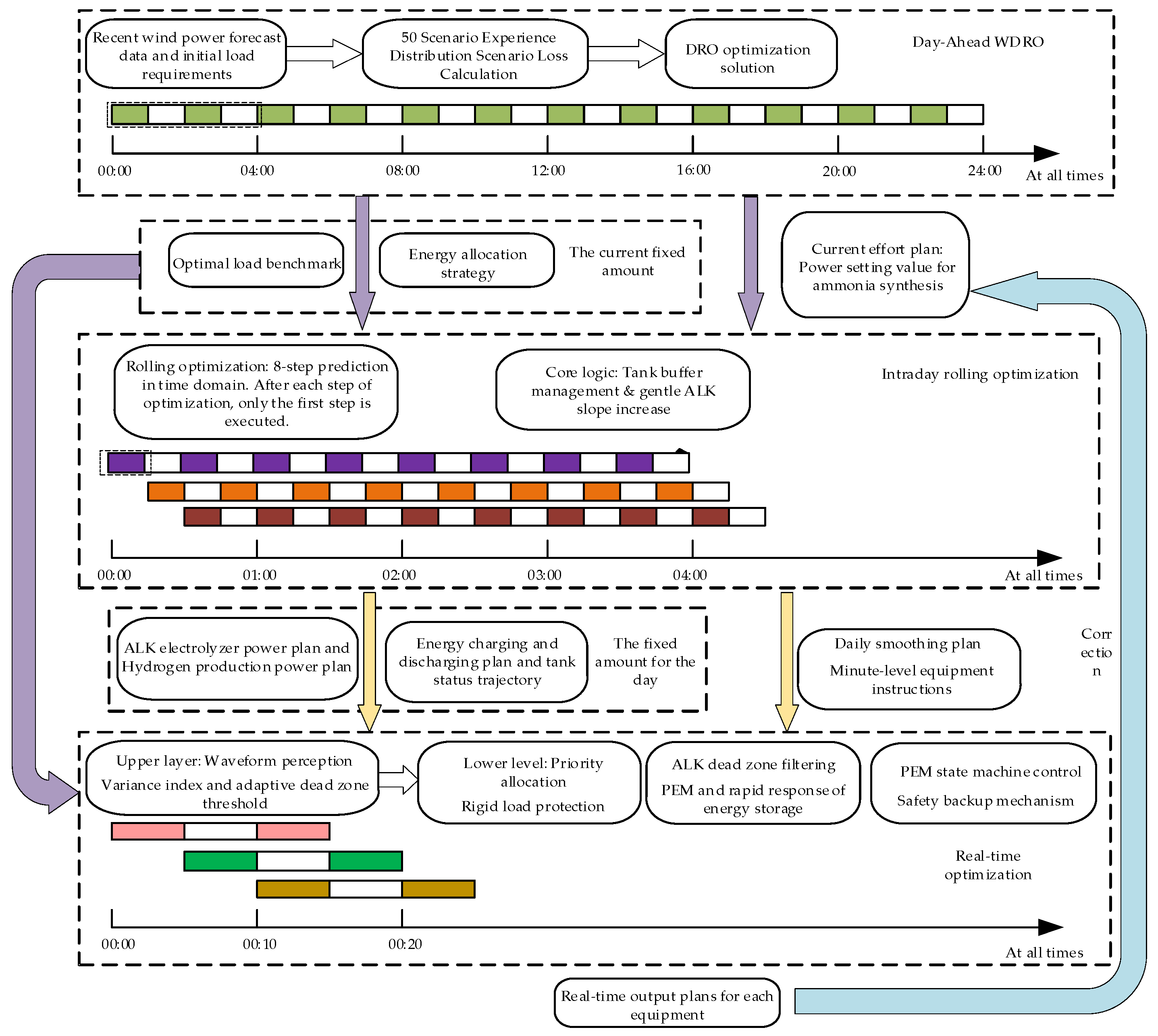
A “day-ahead–intraday–real-time” three-layer coordinated scheduling framework is constructed, as illustrated in Figure 2. This framework adopts a hierarchical optimization approach, with the core philosophy of “rigid protection for ammonia synthesis and flexible regulation of electrolyzers.” This implies treating the ammonia synthesis unit as a stable, rigid load to be protected, while allowing the electrolyzers and energy storage system to absorb all wind and solar fluctuations. While hierarchical control is a standard approach in power systems, the specific internal logic of this framework is an original scheme proposed in this study to address the chemo-physical constraints of ammonia synthesis.

The day-ahead layer is based on WDRO [22], determining a conservative and stable baseline plan for the ammonia load under conditions of highly uncertain wind and solar output. It provides distribution-free statistical guarantees under limited data, making it particularly suitable for long-term planning under highly uncertain renewable forecasts. Unlike traditional stochastic programming, WDRO does not require precise knowledge of the underlying probability distribution, thus avoiding overfitting to noisy historical data while maintaining worst-case robustness. The intraday layer employs MPC with a 2-h prediction horizon and 15-min rolling optimization steps to correct short-term forecast deviations. The real-time layer achieves minute-level power balancing through priority dispatch and deadband control. Furthermore, the hydrogen storage tank acts as a material buffer between hydrogen production and ammonia synthesis, with its state variables passed between layers to achieve flexible multi-time-scale coupling.

The superiority of this architecture stems from its strategic alignment between uncertainty types and decision horizons. Specifically:

• WDRO handles epistemic uncertainty (limited data, unknown distribution) at the strategic level;
• MPC addresses aleatoric uncertainty (random fluctuations) at the tactical level;
• Real-time control manages execution-level noise (measurement error, delays) at the operational level.

This hierarchical design ensures that each layer focuses on its dominant source of uncertainty, avoiding over-conservatism in long-term planning while enabling agile responses in short-term operations. Compared to alternative architectures such as deterministic optimization with post-correction or single-stage robust optimization, this framework offers better trade-offs between robustness, flexibility, and computational tractability.

3.1. Day-Ahead Planning Layer

The objective of the day-ahead planning layer is to formulate a conservative, stable, and executable baseline plan for the ammonia production load under conditions of high uncertainty in renewable energy output.

From a decision-making perspective, the choice of WDRO is driven by the asymmetric risk characteristics of off-grid chemical systems. Traditional stochastic optimization (SO) aims to maximize expected profits based on an assumed ‘perfect’ probability distribution. However, for a rigid ammonia synthesis process, the cost of an unexpected shutdown (due to ‘tail events’ or distribution shifts) far outweighs the benefit of marginal yield increases.

Therefore, the decision-making logic must shift from ‘Expectation-Maximization’ to ‘Ambiguity-Aversion.’ WDRO addresses this by acknowledging that the true distribution of renewable energy is unknown and time-varying due to limited historical data. By constructing a decision plan that remains feasible under the ‘worst-case distribution’ within a statistical confidence set (Wasserstein ball), WDRO provides a conservative ‘Safety Baseline’ for the ammonia load. This ensures operational continuity even when actual weather conditions deviate significantly from historical patterns, reflecting a strategic preference for reliability over theoretical optimality.

WDRO Model

• Problem Modeling

The optimization objective of the day-ahead layer is to minimize the system operating cost under the worst-case probability distribution within a defined Wasserstein ball. The mathematical formulation of the standard WDRO problem is expressed as:

$$\underset{P_{{\mathrm{NH}}_3}^{\mathrm{base}}\in \kappa }{\min }\underset{P\in B_{\vartheta }({\widehat{P}}_{\mathrm{N}})}{\sup }{\mathbb{N}}_P[L(P_{{\mathrm{NH}}_3}^{\mathrm{base}},\xi )].$$

(15)

The definition of the Wasserstein ball is as follows:

$$B_{\vartheta }({\widehat{P}}_{\mathrm{N}})=\{P\in ℝ(\delta ):W_{\mathrm{p}}(P,{\widehat{P}}_{\mathrm{N}})\le \vartheta \}.$$

(16)

Selection of the Wasserstein Radius: The radius of the Wasserstein ball, $\vartheta$, is a critical hyperparameter controlling the robustness of the solution. A radius that is too small implies a lack of robustness against distributional shifts, while a radius that is too large leads to overly conservative solutions and unnecessary economic loss. In this study, instead of relying on loose theoretical bounds which are often too conservative in practice, we employ a data-driven cross-validation approach to calibrate $\vartheta$. The historical data is split into a training set and a validation set. We iterate $\vartheta$ within the range [10⁻³, 10⁻¹] and evaluate the system’s out-of-sample performance. The optimal radius ${\vartheta }^{*}$ is selected as the value that achieves the minimum expected operational cost while satisfying a 95% reliability constraint (i.e., the probability of load shedding is less than 5%) on the validation set.

This data-driven approach is supported by finite-sample guarantees in [23], which prove that the true distribution lies within a Wasserstein ball of radius O(N^−1/d) with high probability. Since this theoretical bound is conservative for high-dimensional settings, the cross-validation procedure above provides a tighter, practically effective estimate of ${\vartheta }^{*}$.

2.

Scenario Generation and Empirical Distribution Construction

The error model parameters are calibrated from one year of paired day-ahead forecast and actual generation data (January–December 2024) collected from the Inner Mongolia station described in Section 4.1. We computed hourly relative forecast errors, defined as $(P_{\mathrm{actual}}-P_{\mathrm{froecast}})/P_{\mathrm{rated}}$, across all 365 days. The errors approximately follow a normal distribution with near-zero mean and standard deviation σ ≈ 0.20 (confirmed by Shapiro–Wilk tests, p > 0.05 for 87% of hourly bins), which directly yields ${\sigma }_{\mathrm{base}}$ = 0.2. A persistent overestimation bias of 5–10% was observed during afternoon hours (13:00–17:00), motivating the uniform bias term with ${\sigma }_{\mathrm{bias}}$ = 0.1. Based on this calibration, 50 typical scenarios are generated as follows:

$$P_{\mathrm{ren},\mathrm{t}}^{\left(\mathrm{s}\right)}=\max \{0,{\widehat{P}}_{\mathrm{ren},\mathrm{t}}\cdot (1+{\epsilon }^{(\mathrm{s})}(t))\},\mathrm{s}=1,2,\dots ,N_{\mathrm{s}},$$

(17)

$${\epsilon }^{\left(\mathrm{s}\right)}(t)={\sigma }_{\mathrm{base}}\cdot \mathbb{N}(0,1)+{\sigma }_{\mathrm{bias}}\cdot (u(0,1)-0.5).$$

(18)

The design of the error model is grounded in two primary considerations: (1) Random Fluctuation Term: This term is employed to characterize the inherent stochastic errors in renewable energy forecasting. The assumption that these errors follow a normal distribution aligns with the statistical properties observed in extensive empirical data [24]. (2) Systematic Bias Term: This term is introduced to capture potential systematic underestimation or overestimation tendencies in the forecasting model. A uniform distribution, rather than a normal distribution, is adopted here. This choice is driven by the high uncertainty regarding the direction and magnitude of the systematic bias; consequently, a uniform distribution provides a more robust and conservative coverage of potential prediction deviations.

3.

Design of a Loss Function Considering Temporal Power Constraints

Conventional Distributionally Robust Optimization (DRO) models often focus solely on the daily global energy balance, neglecting power constraints at individual time steps. In this study, a refined loss function incorporating temporal power constraints is designed to sequentially simulate the system’s operational status under each scenario. Specifically, it comprises penalties for battery SOC violations, hydrogen storage tank terminal constraint penalties, and a comprehensive loss function.

$$L_{SOC}^{(\mathrm{s})}={\displaystyle \sum _{\mathrm{t}=1}^{24}[{\gamma }_{\mathrm{low}}\cdot \max {(0,SO{C}^{\min }-SO{C}_{\mathrm{t}})}^2+{\gamma }_{\mathrm{high}}\cdot \max {(0,SO{C}_{\mathrm{t}}-SO{C}^{\max })}^2]},$$

(19)

$$L_{SOH}^{(\mathrm{s})}={\gamma }_{SOH}\cdot \max {(0,SO{H}^{\min }-SO{H}_{24})}^2,$$

(20)

$$L(P_{{\mathrm{NH}}_3}^{\mathrm{base}},{\xi }^{(\mathrm{s})})=L_{SOC}^{\left(\mathrm{s}\right)}+L_{SOH}^{(\mathrm{s})}-C_{\mathrm{rev}}\cdot P_{{\mathrm{NH}}_3}^{\mathrm{base}}.$$

(21)

For the hydrogen storage tank, a terminal constraint is adopted rather than a cumulative time-series constraint. This is because the hydrogen tank has a large capacity with relatively slow intraday dynamics; thus, ensuring that the storage level at the end of the day is above the safety lower limit is sufficient. The comprehensive loss function aims to maximize ammonia production while accounting for penalties related to SOC and hydrogen tank limit violations. The model prioritizes constraints on the hydrogen tank while simplifying those for the nitrogen tank for the following reasons: (1) The power regulation range of the ASU is narrow, resulting in a relatively stable nitrogen production rate and minimal fluctuations in the nitrogen tank level. (2) The hydrogen-to-nitrogen ratio in ammonia synthesis is fixed at 3:1. Hydrogen supply represents the primary bottleneck of the system; therefore, ensuring the safety of the hydrogen tank indirectly ensures the safety of the nitrogen tank. (3) The nitrogen tank typically possesses a large capacity margin and does not constitute a primary binding constraint within the time scale investigated in this paper.

4.

Solution of the DRO Dual Problem

According to the theoretical findings of Esfahani and Kuhn [22], the WDRO problem can be reformulated into a mean-risk optimization problem via dual transformation. In this study, CVaR is adopted as the risk measure, yielding the following objective function:

$$\underset{P_{{\mathrm{NH}}_3}^{\mathrm{base}}}{\min }\{{\displaystyle \frac{1}{N_{\mathrm{s}}}}{\displaystyle \sum _{\mathrm{s}=1}^{N_{\mathrm{s}}}{L}^{(\mathrm{s})}+\lambda \cdot CVaR}[L]\},$$

(22)

To avoid the non-convexity and computational complexity associated with the direct sorting of scenario losses in the original CVaR definition, we adopt the auxiliary variable method [25] to linearize the risk term. By introducing an auxiliary variable $\chi$ (representing Value-at-Risk) and non-negative variables $z_s$ for each scenario, the CVaR calculation is reformulated as a convex minimization problem:

$$CVaR[L]=\underset{\chi ,z_s}{\min }(\chi +{\displaystyle \frac{1}{[N_{\mathrm{s}}(1-\alpha )]}}{\displaystyle \sum _{\mathrm{i}=1}^{N_{\mathrm{s}}}{z}_s}),$$

(23)

Subject to the following linear constraints:

$$\left\{\begin{array}{l}{z}_s\ge L(P_{{\mathrm{NH}}_3}^{\mathrm{base}},{\xi }^{(\mathrm{s})})-\chi ,\forall s\in \{1,\dots ,N_s\}\\ z_s\ge 0,\forall s\in \{1,\dots ,N_s\}\end{array}\right..$$

(24)

Through this transformation, the comprehensive loss $L(P_{{\mathrm{NH}}_3}^{\mathrm{base}},{\xi }^{(\mathrm{s})})$ is directly embedded into the linear constraints (24). Here, $z_s$ captures the excess loss above the threshold $\chi$ (i.e., $z_s=\max \{L(P_{{\mathrm{NH}}_3}^{\mathrm{base}},{\xi }^{(\mathrm{s})})-\beta ,0\}$). This formulation converts the discrete CVaR calculation into a standard Mixed-Integer Linear Programming form that can be efficiently solved by off-the-shelf solvers (e.g., Gurobi).

Substituting the reformulated CVaR into the original objective, the full DRO problem becomes:

$$J_{\mathrm{DRO}}={\displaystyle \frac{1}{N_{\mathrm{s}}}}{\displaystyle \sum _{\mathrm{s}=1}^{N_{\mathrm{s}}}{L}^{(\mathrm{s})}+\lambda \cdot (\chi +\frac{1}{[N_{\mathrm{s}}(1-\alpha )]}{\displaystyle \sum _{\mathrm{i}=1}^{N_{\mathrm{s}}}{z}_s}}).$$

(25)

Computational Implementation and Efficiency:

In the numerical implementation, the number of historical scenarios is set to $N_s$ = 50. This value was determined through numerical experiments, which indicated that CVaR-based decisions stabilize for $N_s$ ≥ 40, balancing the representativeness of uncertainty with computational tractability.

Regarding the solution technique, the CVaR calculation inherently involves a non-smooth sorting operation. Based on the duality theory of convex optimization, we reformulated this operator into a standard Mixed-Integer Linear Programming (MILP) form using auxiliary variables (Equations (23)–(25)). This transformation is critical: it enables standard MILP solvers to guarantee global optimality, whereas naive implementations of the CVaR operator would require non-convex or combinatorial formulations with significantly higher computational complexity. Consequently, on a standard computing platform (Intel i7-12700H CPU, 16 GB RAM), the day-ahead WDRO model can be solved by the Gurobi solver in less than 40 s. This high efficiency confirms the strategy’s suitability for practical day-ahead scheduling applications.

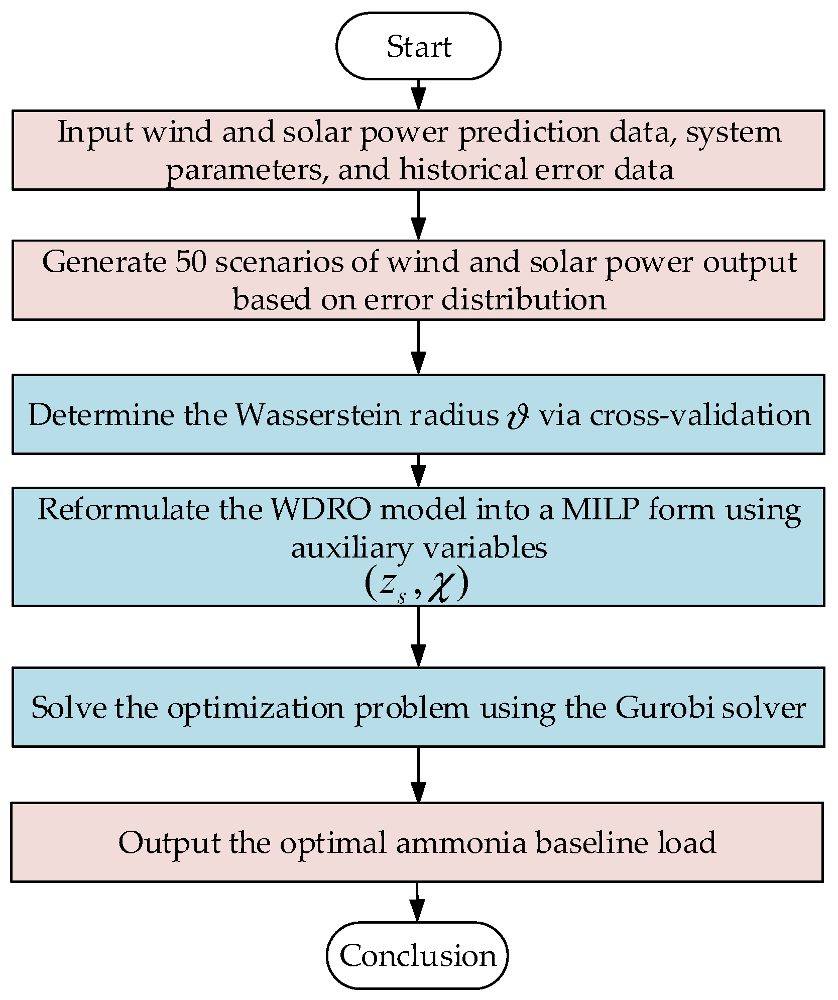
The constructed WDRO model, following the auxiliary variable transformation, essentially constitutes an optimization problem. By minimizing the weighted sum of the expected comprehensive loss and the linearized CVaR term, the model seeks an optimal trade-off between the system’s economic benefits and operational risks. This formulation enables the solver to globally determine an ammonia baseline load instruction that balances profitability with safety boundaries under scenarios of highly uncertain renewable energy output. This results in the generation of a 24-h hourly piecewise constant (step-wise steady state) day-ahead scheduling plan. This plan establishes the ammonia synthesis unit as a ‘rigid load,’ thereby completely decoupling the task of absorbing high-frequency wind and solar fluctuations and allocating it to the electrolyzers and the energy storage system. The computational flowchart of the proposed strategy is shown in Figure 3.

3.2. Intraday Scheduling Layer

The intraday scheduling layer utilizes MPC to perform rolling horizon optimization. The scheduling period consists of 96 time intervals (with a step size of 15 min), the prediction horizon is set to 8 steps (2 h), and the control horizon is 1 step [26]. Its core function is to correct power allocation based on more accurate short-term wind and solar forecasts while tracking the day-ahead plan, thereby ensuring the smooth operation of the load.

The objective function of the intraday layer adopts a multi-objective weighted sum form, aiming to minimize the total cost within the prediction horizon.

$$\underset{\mathrm{u}}{\min }{J}_{\mathrm{MPC}}={\displaystyle \sum _{k=1}^{N_p}(J_{\mathrm{ALK},\mathrm{k}}+J_{{\mathrm{NH}}_3,\mathrm{k}}^{\mathrm{track}}+J_{{\mathrm{NH}}_3,\mathrm{k}}^{\mathrm{smooth}}+J_{SOH,\mathrm{k}}^{\mathrm{bound}})}+J_{\mathrm{terminal}},$$

(26)

$$J_{\mathrm{ALK},\mathrm{k}}=20\cdot {(P_{\mathrm{ALK},\mathrm{k}}-P_{\mathrm{ALK},\mathrm{k}-1})}^2,$$

(27)

$$J_{{\mathrm{NH}}_3,\mathrm{k}}^{\mathrm{track}}=10\cdot {(P_{{\mathrm{NH}}_3,\mathrm{k}}-P_{{\mathrm{NH}}_3,\mathrm{k}}^{\mathrm{DA}})}^2,$$

(28)

$$J_{{\mathrm{NH}}_3,\mathrm{k}}^{\mathrm{smooth}}=100\cdot {(P_{{\mathrm{NH}}_3,\mathrm{k}}-P_{{\mathrm{NH}}_3,\mathrm{k}-1})}^2,$$

(29)

$$J_{SOH,\mathrm{k}}^{\mathrm{bound}}={\omega }_{SOH}^{\mathrm{low}}\cdot \max {(0,0.2-SO{H}_{\mathrm{k}})}^2+{\omega }_{SOH}^{\mathrm{high}}\cdot \max {(0,SO{H}_{\mathrm{k}}-0.9)}^2,$$

(30)

$$J_{\mathrm{terminal}}={\omega }_{SOC}^{\mathrm{end}}\cdot {(SO{C}_{\mathrm{t}+N_p}-SO{C}_{\mathrm{ref}})}^2+{\omega }_{SOH}^{\mathrm{end}}\cdot {(SO{H}^{\mathrm{t}+N_p}-SO{H}^{\mathrm{ref}})}^2.$$

(31)

Parameter Setting Logic: The selection of the weighting coefficients is grounded in the system’s operational priority hierarchy: Process Safety > Equipment Health > Tracking Performance. Specifically, the ammonia fluctuation penalty is assigned the highest weight (100) to strictly restrict the reactor temperature change rate (≤1%/min), reflecting the rigid safety constraints of chemical processes. The electrolyzer smoothing penalty is set to a medium value (20) to limit mechanical stress. The tracking error penalty is set relatively low (10) to provide sufficient flexibility for the controller to utilize energy storage buffering. This ratio design (100:20:10) ensures that the system prioritizes safety boundaries over economic tracking. Furthermore, terminal state constraints are introduced as soft constraints at the end of the prediction horizon to prevent myopic behaviors caused by the rolling optimization nature of MPC.

3.3. Real-Time Scheduling Layer

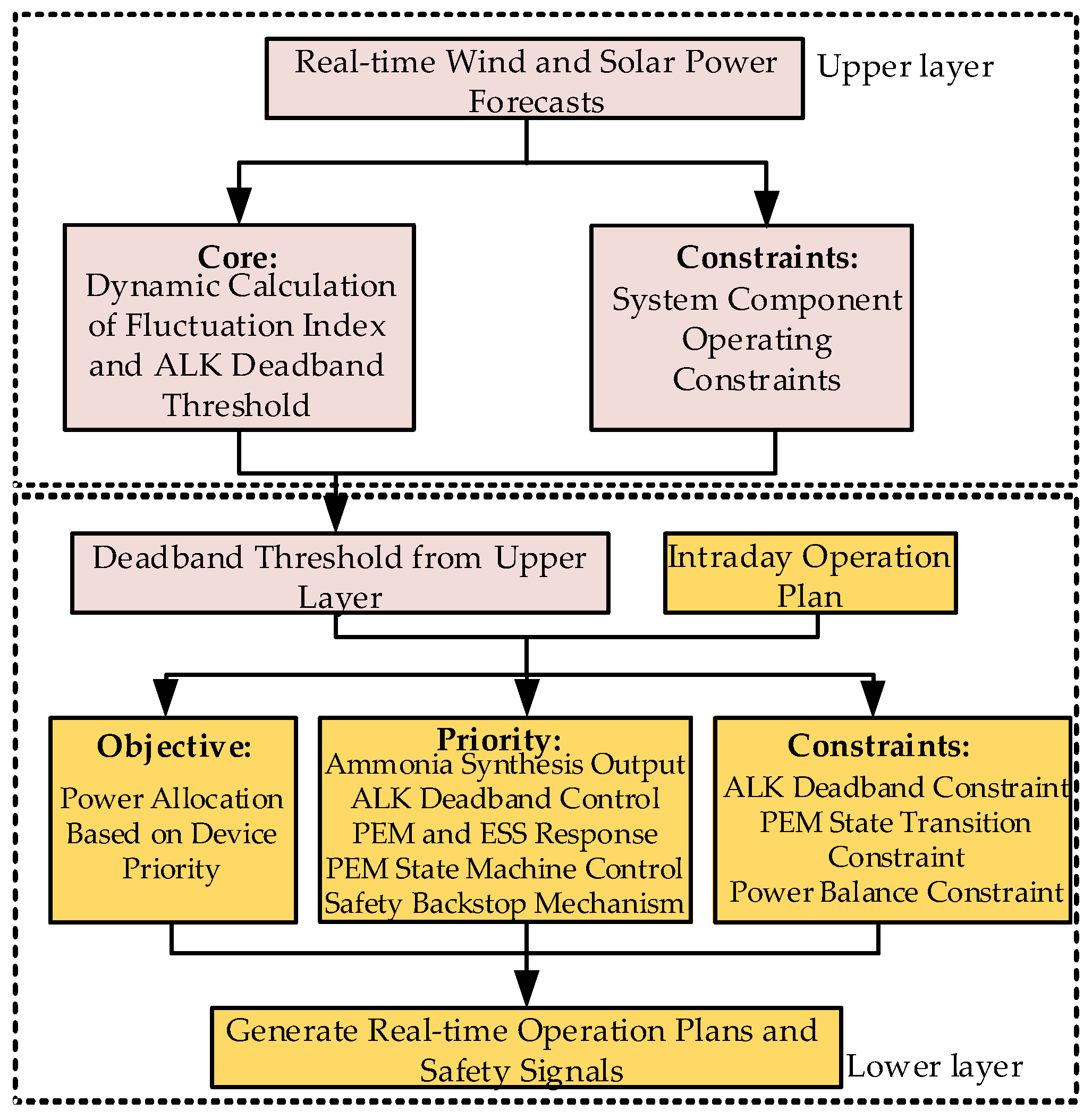
The real-time scheduling layer operates with a control step of 5 min, comprising a total of 288 time periods per day, and adopts a double-layer optimization structure. The upper layer dynamically calculates the regulation deadband threshold of the electrolyzer based on the fluctuation intensity of wind and solar power; the lower layer allocates power according to a priority sequence under these deadband constraints.

Compared with the intraday layer, the real-time layer features a shorter time step, enabling a timelier response to ultra-short-term forecasts of wind and solar power and achieving refined power balancing. Meanwhile, strategies such as deadband control and state machine control are employed to suppress excessive regulation of the equipment, thereby striking a balance between response speed and equipment protection.

3.3.1. Upper-Layer Optimization

The core of the upper-layer optimization is to dynamically adjust the regulation deadband threshold of the ALK according to the fluctuation intensity of the ultra-short-term renewable energy forecasts. First, the fluctuation index within a sliding window is calculated. This fluctuation index is essentially the coefficient of variation, reflecting the relative degree of fluctuation in wind and solar output within a short period. The deadband threshold is then calculated based on this fluctuation index:

$$V{I}_{\mathrm{t}}={\displaystyle \frac{\rho (P_{(\mathrm{t}-\Delta w:\mathrm{t})})}{\mu (P_{(\mathrm{t}-\Delta w:\mathrm{t})})+\phi }},$$

(32)

$${\theta }_{\mathrm{t}}=P_{\mathrm{ALK}}^{\mathrm{rated}}\cdot {\theta }_0\cdot (1+l_{VI}\cdot V{I}_{\mathrm{t}}).$$

(33)

When wind and solar fluctuations are intense, the deadband is expanded to suppress frequent regulation of the electrolyzer; when fluctuations are stable, the deadband is narrowed to improve tracking accuracy. Here, the base deadband (0.02) is selected to filter out measurement noise (typically < 1%), and the coefficient (8) is calibrated to ensure the deadband covers the ALK’s ramp-rate limit under high fluctuation intensity.

Regarding the enforcement of the ramp-rate constraint (≤1%/min) across layers: in the intraday layer ($\Delta t$ = 15 min), this constraint is equivalently imposed as |ΔP_NH3| ≤ 15% of rated power per step, corresponding to $\Delta \max$ in Equation (7). In the real-time layer ($\Delta t$ = 5 min), it tightens to ≤5% per step. Moreover, since the ammonia unit is locked to the intraday command via Equation (34) and is not adjusted at the minute level, the ramp constraint is inherently satisfied in real-time execution

Boundary behavior of the deadband: (i) When renewable output is steady ($V{I}_{\mathrm{t}}$ → 0), the deadband reduces to its base value ${\theta }_0$·$P_{\mathrm{ALK}}^{\mathrm{rated}}$ = 0.02 × 70.1 ≈ 1.4 MW, sufficient to filter measurement noise. (ii) Under extreme volatility ($V{I}_{\mathrm{t}}$ → 1), the deadband expands to approximately 0.02 × (1 + 8) × 70.1 ≈ 12.6 MW, which remains within the ALK’s operating range [$P_{\min }$, $P_{\max }$] and is comparable to its 5-min ramp capacity (1%/min × 70.1 MW × 5 min ≈ 3.5 MW), ensuring that only fluctuations exceeding the physical ramp capability trigger re-dispatch. (iii) During zero renewable output, the system enters the emergency protection mode (Section 3.3.2 (5)), bypassing the deadband logic entirely.

3.3.2. Lower-Layer Optimization

The lower-layer optimization adopts a rule-based priority dispatch strategy. The strategy is executed in the following sequence: “rigid load guarantee—ALK smooth following—hybrid energy storage fluctuation suppression—safety backstop mechanism.”

(1)

Rigid Load Protection

The real-time layer treats the ammonia synthesis unit as a rigid load, prioritizing the satisfaction of the rolling power command from the intraday layer without performing real-time adjustments. This ensures the maintenance of the thermal balance within the synthesis reactor tower:

$$P_{{\mathrm{NH}}_3,\mathrm{t}}=P_{{\mathrm{NH}}_3,\mathrm{t}}^{\mathrm{ID}}.$$

(34)

(2)

ALK Deadband Filtering

The ALK undertakes baseload consumption and filters high-frequency fluctuations through deadband control. When power fluctuations fall within the deadband, the ALK maintains its output from the previous time step to reduce mechanical wear; when fluctuations exceed the deadband, the ALK only undertakes the low-frequency components, subject to maximum ramp rate constraints:

$$P_{\mathrm{ALK},\mathrm{t}}^{\mathrm{target}}=\left\{\begin{array}{l}{P}_{\mathrm{ALK},\mathrm{t}-1},\mathrm{if}\left|\Delta P_{\mathrm{t}}\right|<{\theta }_{\mathrm{t}}\\ P_{\mathrm{ALK},\mathrm{t}-1}+\mathrm{sign}(\Delta P)\cdot \Delta P_{\max },\mathrm{otherwise}\end{array}\right..$$

(35)

To balance “fluctuation suppression” and “intraday plan tracking,” the expected power reference value for the ALK is calculated:

$$P_{\mathrm{ALK},\mathrm{t}}^{\mathrm{ref}}={\alpha }_{DB}\cdot P_{\mathrm{ALK},\mathrm{t}}^{\mathrm{target}}+(1-{\alpha }_{DB})\cdot P_{\mathrm{ALK},\mathrm{t}}^{\mathrm{ID}}.$$

(36)

However, due to the lack of grid support in the off-grid system, if renewable energy output drops suddenly while the intraday plan remains high, blind execution of the reference value would lead to system collapse. Therefore, a real-time available power check mechanism is introduced to generate the final command:

$$P_{\mathrm{ALK},\mathrm{t}}=\min \{P_{\mathrm{ALK},\mathrm{t}}^{\mathrm{ref}},P_{\mathrm{ren},\mathrm{t}}+P_{\mathrm{bat}}^{\mathrm{dmax}}\cdot {\eta }_{\mathrm{bat}}-P_{{\mathrm{NH}}_3,\mathrm{t}}\}.$$

(37)

This mechanism ensures that the ALK is regulated only within the range permitted by the system’s power supply capability.

(3)

Rapid Response of PEM and Energy Storage

Since the ALK cannot fully track high-frequency fluctuations in wind and solar power due to ramp rate and deadband limitations, the resulting power shortage must be jointly undertaken by the PEM and the lithium battery, which possess superior dynamic characteristics. First, the real-time power imbalance is defined as the difference between the ultra-short-term forecasted renewable energy output and the “rigid” loads:

$$\Delta P_{\mathrm{net},\mathrm{t}}=P_{\mathrm{ren},\mathrm{t}}^{\mathrm{pred}}-P_{{\mathrm{NH}}_3,\mathrm{t}}-P_{\mathrm{ASU},\mathrm{t}}-P_{\mathrm{ALK},\mathrm{t}}.$$

(38)

This imbalance is allocated according to the following logic:

A. PEM Fast Response

Leveraging its fast response characteristics, the PEM prioritizes the absorption of positive power surplus, subject to adaptive start-up threshold constraints:

$$P_{\mathrm{PEM},\mathrm{t}}=\left\{\begin{array}{c}\max (P_{\mathrm{PEM}}^{\min },\min (\Delta P_{\mathrm{net},\mathrm{t}},P_{\mathrm{PEM}}^{\max })),\mathrm{if}\Delta P_{\mathrm{net},\mathrm{t}}\ge \max (P_{\mathrm{start}},P_{\mathrm{PEM}}^{\min })\\ 0,\mathrm{if}\Delta P_{\mathrm{net},\mathrm{t}}<P_{\mathrm{start}}\mathrm{or}\Delta P_{\mathrm{net},\mathrm{t}}<P_{\mathrm{PEM}}^{\min }\end{array}\right..$$

(39)

B. Battery Energy Storage

As the final regulation means of the system, the battery output power is the superposition of the intraday energy plan and the real-time fluctuation smoothing component:

$$\left\{\begin{array}{c}{P}_{\mathrm{bat},\mathrm{t}}=P_{\mathrm{bat},\mathrm{t}}^{\mathrm{ID}}+\Delta P_{\mathrm{bat},\mathrm{t}}^{\mathrm{adj}}\\ \Delta P_{\mathrm{bat},\mathrm{t}}^{\mathrm{adj}}=\Delta P_{\mathrm{net},\mathrm{t}}-P_{\mathrm{PEM},\mathrm{t}}\end{array}\right..$$

(40)

When the real-time smoothing power is positive, the battery absorbs the residual surplus caused by insufficient PEM capacity; when negative, the battery discharges rapidly to bridge the power gap caused by sudden drops in wind and solar power, supporting bus voltage stability. Finally, the battery power must satisfy capacity constraints:

$$-P_{\mathrm{bat}}^{\mathrm{dmax}}\le P_{\mathrm{bat},\mathrm{t}}\le P_{\mathrm{bat}}^{\mathrm{cmax}}.$$

(41)

(4)

PEM Adaptive State Machine Control

To avoid frequent start-stop cycles of the PEM, an adaptive hysteresis control strategy based on the hydrogen tank level is adopted. The start-up threshold is dynamically adjusted as follows:

$$P_{\mathrm{PEM},\mathrm{t}}^{\mathrm{on}}=P_{\mathrm{PEM}}^{\mathrm{rated}}\cdot ({\beta }_{\mathrm{on}}^{\mathrm{base}}-{\beta }_{\mathrm{on}}^{\mathrm{adj}}\cdot {\displaystyle \frac{SO{H}_{\mathrm{t}}-0.5}{0.5}}).$$

(42)

When the hydrogen tank level is below 0.5, the start-up threshold is lowered to facilitate PEM start-up for supplementary hydrogen production; when the level is above 0.5, the threshold is raised to reduce unnecessary start-ups.

(5)

Safety Backstop Mechanism

Curtailment Mode: When renewable energy surges, the ALK is locked by the deadband, the PEM is fully loaded, and the battery SOC reaches its upper limit, renewable energy curtailment is triggered to ensure bus voltage stability.

Emergency Load Shedding: When renewable energy drops suddenly, the battery SOC touches its lower limit, and the hydrogen tank level is critically low, an emergency protection mechanism is triggered to forcibly shed part of the ammonia synthesis load.

The specific flowchart of the double-layer optimization in the real-time stage is shown in Figure 4.

3.4. Time-Scale-Specific Implementation of Ramp-Rate Constraints

The ramp-rate constraint for the ammonia synthesis unit is strictly enforced to ensuring operational safety. As defined in Section 2.2.3, the base physical constraint is ≤1% of the rated capacity per minute. In the proposed optimization framework, this continuous physical limit is discretized and adapted to the time resolution of each scheduling layer as follows:

• Intraday Layer ($\Delta t$ = 15 min): The constraint is integrated into the MPC rolling optimization. The allowable power adjustment per time step is calculated as 1%/min × 15 min = 15%. Thus, the constraint imposed on the decision variables is:

  $$|P_{{\mathrm{NH}}_3,\mathrm{t}}-P_{{\mathrm{NH}}_3,\mathrm{t}-1}|\le 0.15\cdot P_{{\mathrm{NH}}_3}^{\mathrm{rated}},\hspace{1em}\forall t.$$

  (43)
• Real-time Layer ($\Delta t$ = 5 min): For the finer real-time dispatch, the constraint is tightened strictly to:

  $$|P_{{\mathrm{NH}}_3,\mathrm{t}}-P_{{\mathrm{NH}}_3,\mathrm{t}-1}|\le 0.05\cdot P_{{\mathrm{NH}}_3}^{\mathrm{rated}},\hspace{1em}\forall t.$$

  (44)
• Linearization for MILP Solving: To maintain the convexity and computational tractability of the optimization model, the absolute value term in the ramp-rate constraint is reformulated into two linear inequality constraints:

  $$P_{{\mathrm{NH}}_3,\mathrm{t}}-P_{{\mathrm{NH}}_3,\mathrm{t}-1}\le \Delta P_{{\mathrm{NH}}_3}^{\max },$$

  (45)

  $$P_{{\mathrm{NH}}_3,\mathrm{t}-1}-P_{{\mathrm{NH}}_3,\mathrm{t}}\le \Delta P_{{\mathrm{NH}}_3}^{\max }.$$

  (46)

Here, $\Delta P_{{\mathrm{NH}}_3}^{\max }$ takes the value of $0.15\cdot P_{{\mathrm{NH}}_3}^{\mathrm{rated}}$ for the intraday layer and $0.05\cdot P_{{\mathrm{NH}}_3}^{\mathrm{rated}}$ for the real-time layer. This reformulation allows the model to be efficiently solved by standard Mixed-Integer Linear Programming (MILP) solvers without introducing additional binary variables.

3.5. Inter-Layer Coordination Mechanism

The three-layer scheduling framework achieves coordination through the following mechanisms:

3.5.1. Information Downlink

The upper layer transmits the power baseline trajectory to the lower layer. The day-ahead layer outputs hourly-level piecewise constant load values. On the basis of tracking this trajectory, the intraday layer utilizes rolling optimization to perform smoothing processing on time-period transitions or to correct the ammonia synthesis plan under extreme deviations. The real-time layer then regards the final command issued by the intraday layer as a rigid target to be strictly executed, without performing frequent minute-level adjustments.

3.5.2. State Feedback

The lower layer feeds back the actual operating status to the upper layer. The hydrogen storage level is fed back to the intraday layer for objective function updates and simultaneously to the real-time layer for the dynamic adjustment of PEM control parameters, forming a closed-loop control.

3.5.3. Flexible Coupling

The hydrogen storage tank provides a material buffer between hydrogen production and ammonia synthesis. When the hydrogen tank storage level is at 50%, it can support the independent operation of the ammonia synthesis unit for approximately 8~10 h. This substantial material buffer capacity not only achieves time decoupling between the hydrogen production and consumption links but also provides a generous regulation window for the intraday MPC, enabling it to cope effectively with drastic intraday fluctuations or even short-term interruptions in renewable energy output.

3.5.4. Emergency Protection

When the battery SOC drops below 0.05 and the hydrogen storage tank level falls below 0.1, a protection mechanism is triggered. This mechanism authorizes the shedding of the ammonia synthesis load to prevent system collapse.

4. Case Analysis

4.1. Case Parameter Settings

This study utilizes data from a wind farm and a photovoltaic power station in a specific region of Inner Mongolia as a case study, assuming the average daily demand for green ammonia is 80 t/day. The optimization results of the system are analyzed based on the following configuration: 80 MW of wind power units, 60 MW of photovoltaic units, a 40 MWh lithium-ion battery pack, a 70.1 MW ALK electrolyzer, a 20.2 MW PEM electrolyzer, a 2500 m³ spherical hydrogen storage tank group (at 5 MPa), and a 300 m³ nitrogen storage tank.

The upper and lower limits of the SOC for the lithium-ion battery are set to 0.9 and 0.1, respectively, with an initial SOC of 0.5. Referencing current market trends for the green ammonia premium, the sales price of green ammonia is set at 4000 CNY/t. The load shedding penalty coefficient, which accounts for economic losses such as catalyst degradation, feedstock venting, and restart costs, is calculated as five times the sales price. The simulation environment utilized in this study is MATLAB R2021b(MathWorks, Inc., Natick, MA, USA), running on a 12th Gen Intel(R) Core(TM) i7-12700H CPU (Intel Corporation, Santa Clara, CA, USA) with 16 GB of RAM. The Gurobi optimizer (version 9.5.2, Gurobi Optimization, LLC, Beaverton, OR, USA) is employed to solve the optimization model.

The simulation results presented in this section are derived from the rigorous implementation of the refined mathematical model detailed in Section 2 and Section 3. Specifically, the optimization framework strictly enforces the formalized ammonia ramp-rate constraints (Equation (7)) and incorporates the linearized CVaR formulation (Equation (25)) to ensure that the numerical outcomes fully reflect the proposed safety mechanisms and computational efficiency.

4.2. Economic and Robustness Advantages of Day-Ahead WDRO

High-precision minute-level time series were constructed based on actual wind and solar data, and typical forecast errors (such as a sudden drop scenario in the afternoon) were introduced to simulate uncertainty in a realistic operating environment. To comprehensively evaluate the performance, the following three comparative scenarios are established:

Scenario 1: A control strategy based on deterministic day-ahead optimization and real-time source-following-load logic.

Scenario 2: A control strategy based on day-ahead Stochastic Optimization (SO) combined with intraday rolling MPC.

Scenario 3: The multi-time-scale optimization scheduling strategy proposed in this paper, based on “Day-ahead DRO–Intraday MPC–Real-time Deadband Control.”

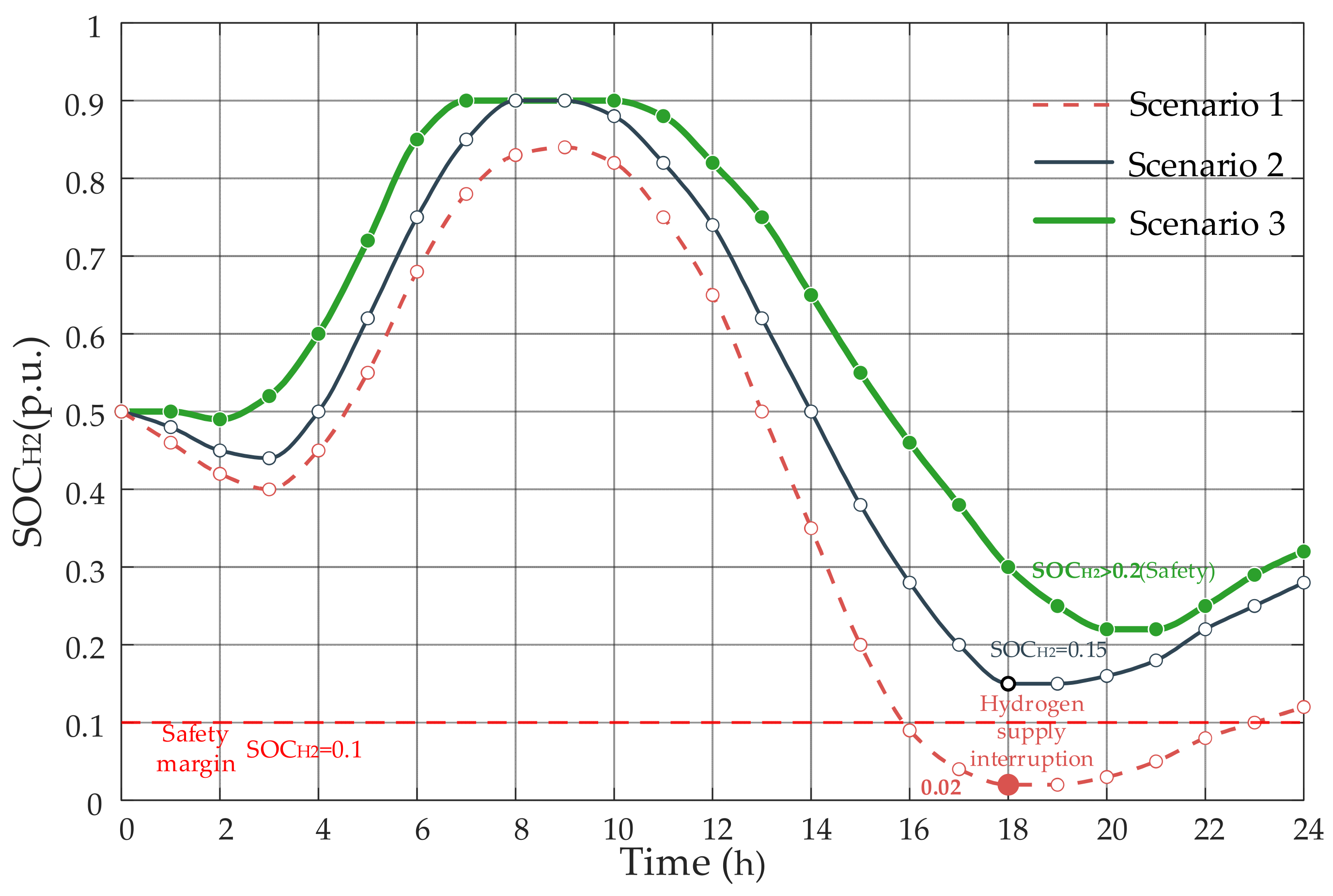
As shown in Figure 5, under highly uncertain renewable output, the hydrogen storage dynamics exhibit distinct behaviors across scenarios.

Scenario 1 relies heavily on point forecasts, resulting in an overly aggressive ammonia load baseline of 50 MW. When actual wind and solar output sharply declined after 13:00, the hydrogen tank’s SOC dropped rapidly below the safety threshold (SOC_H2 = 0.1), approaching a critical state of hydrogen supply interruption.

Scenario 2, although incorporating uncertainty via scenario-based SO, adopts a risk-neutral objective that minimizes expected cost. This leads to insufficient safety margins: the SOC reaches a minimum of 0.15, indicating vulnerability under extreme conditions.

In contrast, Scenario 3 employs WDRO to explicitly account for distributional ambiguity. It proactively reduces the load baseline to 43 MW (a 14% reduction), reserving ample buffer capacity. Even under worst-case fluctuations, the SOC_H2 remains above 0.2 throughout the day, demonstrating superior robustness and complete avoidance of load shedding.

As shown in

Table 2. Daily and annual operating costs of the system.

Cost Component	Scenario 1	Scenario 2	Scenario 3
Theoretical Daily Production(t)	82.5	80.0	80.0
Actual Daily Production(t)	68.2	75.5	80.0
Daily Ammonia Sales Revenue(CNY)	273,000	302,000	320,000
Daily O&M Cost(CNY)	38,600	40,100	42,300
Penalty Cost(CNY)	386,000	50,000	0
Daily Net Profit(CNY)	−151,600	211,900	277,700
Annual Actual Production (t)	22,703	23,453	28,494
Annual Load-shedding Penalty (104 CNY)	12,533.33	2933.33	0.00
Annual Net Profit (104 CNY)	−3906.20	5978.75	10,827.61
Annual Load-shedding Events (times)	12	4	0
SOCH2 Violation Duration (h/yr)	23.5	5.5	0

, On a daily basis, Scenario 1 incurs a net loss of −151,600 CNY due to high penalty costs (386,000 CNY). Scenario 3 achieves a daily net profit of 277,700 CNY with zero penalties—representing an absolute profit improvement of 429,300 CNY compared to Scenario 1.

Annually, the advantages of Scenario 3 are even more pronounced. Scenario 1 experiences 12 load-shedding events and 23.5 h of SOC_H2 violations, leading to a total annual deficit of −3.906 × 10⁴ CNY. Scenario 2 improves this to 4 load-shedding events and 5.5 h of violation, achieving a net profit of 5.979 × 10⁴ CNY. However, Scenario 3 eliminates all load shedding and SOC_H2 violations entirely, realizing an annual net profit of 10.828 × 10⁴ CNY—an increase of 4.849 × 10⁴ CNY over Scenario 2 and a remarkable turnaround from deficit to profitability compared to Scenario 1.

Beyond the numerical disparities, these results expose a fundamental difference in control philosophy between the strategies:

• Fragility of Deterministic Logic: Scenario 1 fails because it treats the point forecast as ground truth. In off-grid systems, the absence of grid inertia means any forecast error directly impacts the rigid load. Deterministic optimization lacks the mathematical structure to reserve ‘uncertainty margins,’ making it structurally unsuitable for islanded chemical plants.
• Short-sightedness of Risk-Neutrality: Although Scenario 2 considers uncertainty, its objective function minimizes the expected value (mean cost). This risk-neutral approach implicitly assumes that ‘under-production’ and ‘over-production’ are symmetric risks. However, for ammonia synthesis, the risk is highly asymmetric: a power shortage leads to a costly shutdown, while a surplus only causes minor curtailment. Stochastic optimization fails to capture this asymmetry, resulting in insufficient safety buffers (low SOC).
• Robustness of Distributional Ambiguity: Scenario 3 succeeds by shifting the paradigm to Ambiguity-Aversion. By optimizing against the worst-case distribution (WDRO), it effectively places a high penalty on the ‘tail risk’ of power shortages. This mechanism forces the solver to sacrifice a fraction of the theoretical peak yield (the 14% baseline reduction) to purchase an actual guarantee of continuity. This proves that in off-grid chemical engineering, reliability is the prerequisite for profitability.

These results validate a core engineering principle: operational reliability is not merely a technical requirement but the foundation of economic efficiency.

4.3. Comparative Analysis of Ammonia Load Fluctuation Characteristics

Under the aforementioned scenarios, the capabilities of the three strategies in regulating ammonia load fluctuations are compared.

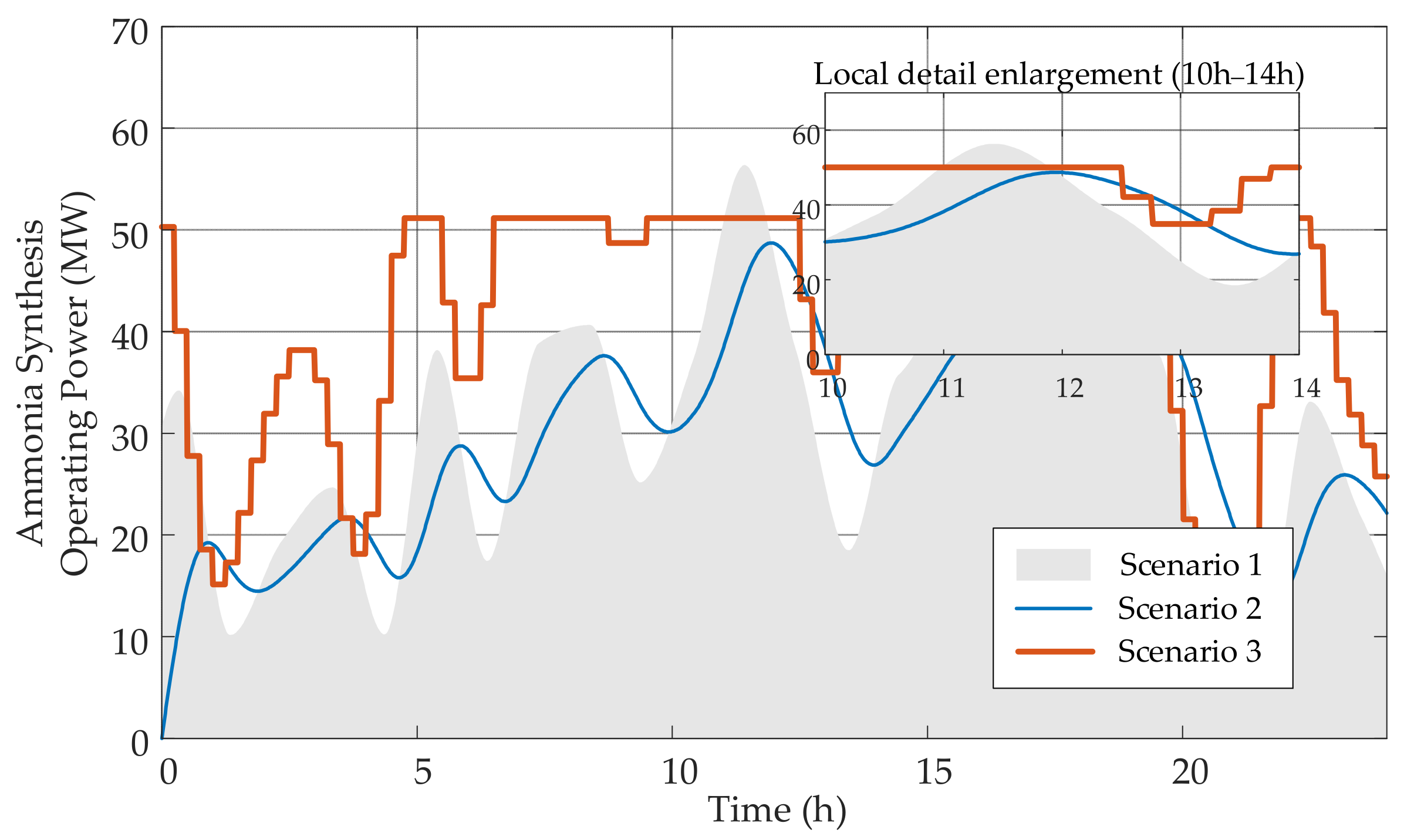
Figure 6 illustrates the operating power curves of the ammonia synthesis unit under each strategy over a full 24-h period. The morphological differences among the three curves profoundly reveal the control effects of different scheduling mechanisms.

The gray shaded area represents Scenario 1. Here, the actual renewable energy output is converted proportionally to the maximum ammonia power without any regulation mechanism. Consequently, the ammonia power is forced to follow the wind and solar output with violent second-level fluctuations. The peak-to-valley difference exceeds 50 MW, which, in engineering practice, would lead to thermal runaway of the catalyst bed, failing to meet the requirements for continuous chemical production. The blue solid line represents Scenario 2. Relying on energy storage buffering, it possesses a certain smoothing capability but exhibits significant response lag. At the sudden change point of 13:00, due to a lack of foresight regarding the future drop, the load decreases slowly. This leads to the rapid depletion of energy storage, facing a severe risk of over-discharge and suffering from the issue of “frequent operating condition changes.” The orange staircase line represents the power curve generated by the proposed strategy (Scenario 3). It presents unique “step-wise steady state” characteristics, reflecting the synergistic effect of the three-layer architecture. The curve overall exhibits an hourly piecewise constant shape, indicating that the system strictly follows the robust baseline formulated by the day-ahead DRO, effectively shielding against minute-level high-frequency interference.

Notably, in the magnified view (10:00–14:00), focusing on the 12:00–13:00 period, although the actual wind and solar output had not yet hit bottom, the orange curve lowered the power from 50 MW to 30 MW one hour in advance and locked it. This is a typical feature of intraday MPC rolling optimization—the controller predicted an energy gap in the coming 2 h and thus commanded the system to “shed load in advance” to preserve the hydrogen tank level, avoiding a cliff-like shutdown in subsequent moments. Within the steps (e.g., 10:00–12:00), despite intense fluctuations in wind and solar output, the ammonia power remained at an absolute level. This validates the effectiveness of the real-time layer’s “deadband control,” successfully isolating source-side fluctuations from the chemical process. This effectively avoids extreme operating conditions caused by inaccurate predictions and significantly enhances the system’s disturbance rejection capability and operational safety.

4.4. Analysis of Energy Storage Synergistic Characteristics

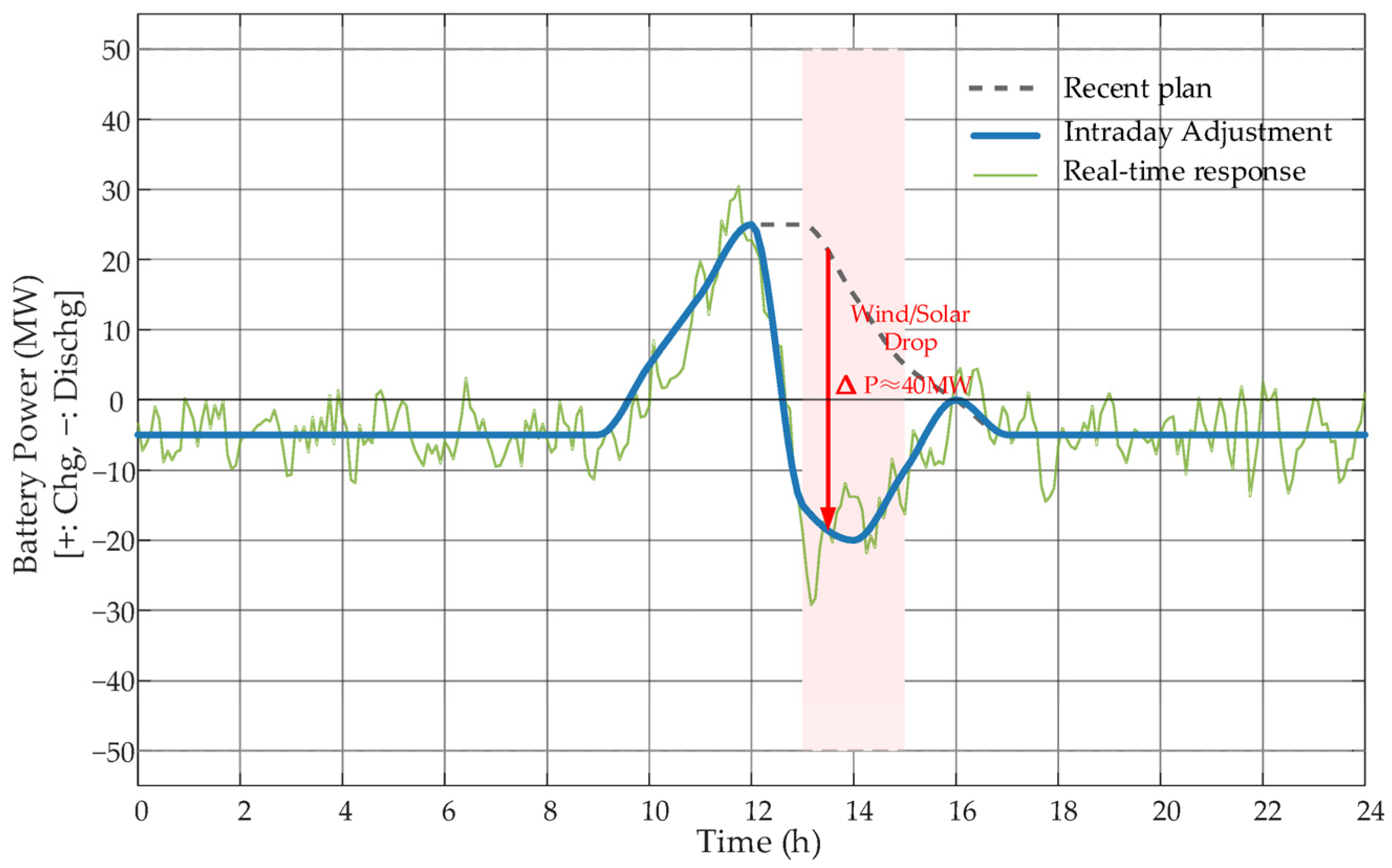
As shown in Figure 7, the energy storage charge/discharge plan presents a smooth baseload shape on the day-ahead scale, primarily used for peak shaving and valley filling to ensure daily energy balance. Its depth of charge/discharge is strictly limited to reserve regulation capability for intraday uncertainties. In the intraday correction phase, MPC rolling optimization performs refined corrections to the day-ahead plan based on 2-h short-term forecasts. During the 13:00–15:00 wind/solar drop window, the energy storage rapidly switched from a “charging” state to a “discharging” state, boosting power by approximately 20 MW. This effectively smoothed the downward slope of the ammonia load, embodying the philosophy of preventive regulation. On the real-time scale, energy storage undertakes the backstop task for high-frequency fluctuations. When the ALK electrolyzer cannot respond to second-level fluctuations due to deadband and ramp rate constraints, the battery performs rapid charging and discharging with a 5-min step size. Although the power fluctuation amplitude reaches ±15 MW, the duration is short, avoiding drastic oscillations in the SOC.

4.5. Analysis of Flexible Division of Labor and Equipment Protection for Electrolyzers

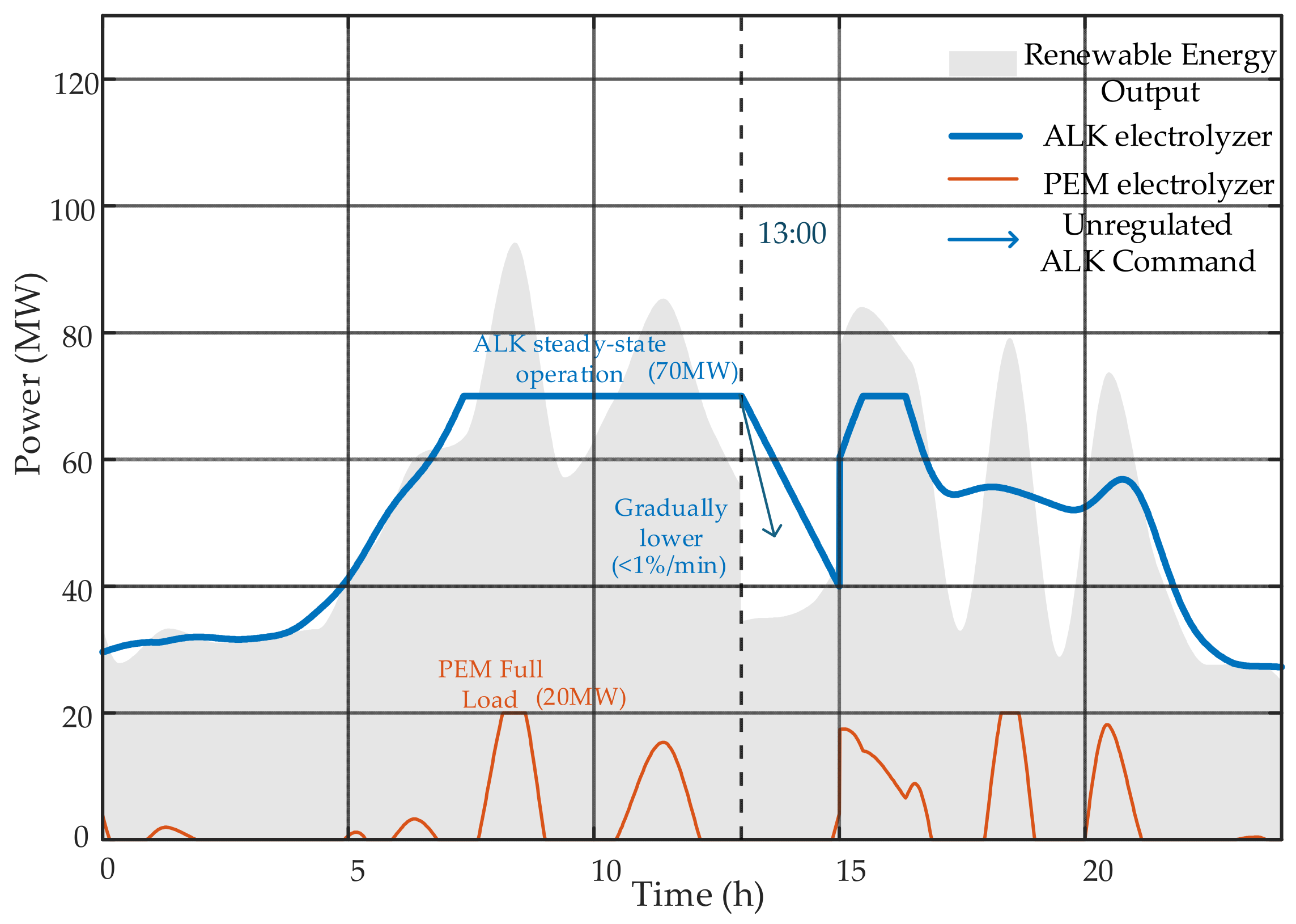
As shown in Figure 8, the simulation results clearly demonstrate the “role allocation” and “dynamic coordination” mechanisms of the two types of electrolyzers under the multi-time-scale coordination strategy. The thick blue solid line indicates that the ALK undertakes the vast majority of the hydrogen production tasks, with its power curve exhibiting significant smoothness and lag. During the high wind and solar output period of 08:00–13:00, the ALK operated stably near its rated condition of 70 MW. This not only ensured high-efficiency hydrogen production but also avoided efficiency decay caused by frequent condition changes through long-term stable operation. At the 13:00 sudden drop moment, the raw power demand command (indicated by the thin blue line) showed a cliff-like drop. If this command were executed directly, it would cause a “trip” risk for the ALK. However, under the action of real-time deadband control and ramp rate limits (Constraint < 1%/min), the actual ALK power did not plummet with the command but instead performed a linear downward adjustment with a gentle slope. This “time-for-space” control strategy effectively curbed the mechanical impact of power mutations on the electrolyzer diaphragm. The orange solid line represents the operating power of the PEM. Unlike the “sluggishness” of the ALK, the PEM exhibited extreme sensitivity, precisely capturing the high-frequency residual power that the ALK could not respond to. At moments like 11:00 and 19:00, when wind and solar output spiked (exceeding the ALK ramp capability), the PEM started up rapidly and instantly reached full load. Throughout the day, the PEM displayed multiple “pulse-like” operating characteristics. This validates the PEM’s role as a “fluctuation absorber,” where its response speed perfectly compensates for the dynamic deficiencies of the ALK. By comparing the blue and orange lines, it can be seen that the proposed strategy successfully achieves spectrum separation of source-side fluctuations: the ALK is responsible for responding to hour-level low-frequency energy blocks, while the PEM is responsible for responding to minute-level high-frequency glitches. This “rigid–flexible coupling” combination not only leverages the low-cost advantage of the ALK but also utilizes the PEM to ensure the dynamic balance of the system, maximizing the operational lifespan of core equipment to the greatest extent.

4.6. Parameter Sensitivity Analysis and Ablation Study

To verify the robustness of the parameter selection and the necessity of each objective term in the MPC optimization, we conducted a systematic sensitivity analysis and an ablation study.

4.6.1. Sensitivity Analysis of Weight Coefficients

We varied the key penalty weights for electrolyzer smoothing and ammonia smoothing within a range of ±50% relative to their baseline values. The impact of these variations on the system’s economic performance and operational stability is presented in

Table 3. Sensitivity analysis of key MPC weights.

Case ID	Electrolyzer Smoothing	Ammonia Smoothing	Daily Net Profit (104 CNY)	Load Shedding Events
Baseline	20	100	27.7	0
Case 1	10	100	27.15	0
Case 2	20	50	26.42	0
Case 3	30	50	25.18	2

.

As shown in Table 3, the system demonstrates strong economic robustness, with the Daily Net Profit fluctuating within a narrow range across different parameter combinations. Notably, the baseline strategy achieves the highest net profit across all tested configurations, indicating its superiority within the explored parameter space. This result suggests that the selected weight combination strikes an optimal balance between economic efficiency and operational constraints. In contrast, reducing the electrolyzer smoothing penalty (Case 1) leads to a profit decrease to 27.15 × 10⁴ CNY. This counter-intuitive result occurs because excessive power fluctuations in the electrolyzer force the battery system to undergo frequent charge/discharge cycles to maintain bus balance, thereby increasing operational costs and energy losses [27].

Regarding operational safety, the penalty weight for ammonia smoothing plays a decisive role in maintaining system stability [28]. When ammonia smoothing is maintained at a high level (100, as in Baseline and Case 1), the system consistently achieves zero load shedding. However, when the protection strength for ammonia is significantly weakened (Case 3) combined with a stricter constraint on the electrolyzer, the system fails to absorb extreme fluctuations effectively, resulting in 2 load-shedding events and a significant profit drop. This validates that a high penalty weight for ammonia smoothing is essential to uphold the “rigid load” safety characteristic.

4.6.2. Ablation Study

To validate the specific contribution of each constraint in the multi-objective function, we conducted an ablation study by sequentially removing penalty terms. The comparative results are summarized in

Table 4. Ablation study results of the MPC objective function.

Exp. ID	Removed Term	Daily Net Profit (104 CNY)	Ammonia Fluctuation (MW)
Baseline	None (Full Model)	27.7	0.99
Exp. A1	w/o Ammonia Smoothing	23.24	3.47
Exp. A2	w/o Terminal Constraint	23.57	1.45
Exp. A3	w/o Electrolyzer Smooth	26.35	1.24

.

The results in Table 4 reveal the distinct and critical role of each objective term.

First and foremost, the ammonia smoothing term is identified as the cornerstone of system safety. Removing this term (Exp. A1) results in the most severe economic impact, causing a daily profit loss of 4.53 × 10⁴ CNY compared to the baseline. More critically, this loss of “rigid” protection directly triggers load-shedding events, confirming that strict constraints on ammonia load fluctuations are non-negotiable for safe chemical production.

Secondly, the terminal constraints prove essential for ensuring the continuity of long-term operation. Without these constraints (Exp. A2), the MPC controller exhibits “myopic” behavior, exhausting energy storage resources at the end of the day to minimize immediate costs. This phenomenon is consistent with known limitations of receding-horizon control without terminal constraints in energy systems [29]. While some recent studies have incorporated such constraints to improve long-term feasibility [30], they remain underutilized in green ammonia scheduling frameworks. This leads to a profit loss of 4.20 × 10⁴ CNY and causes SOC violations, leaving the system vulnerable for the subsequent operating cycle.

Finally, the comparison with Exp. A3 highlights the synergistic effect of the proposed framework. While removing the electrolyzer smoothing term results in a relatively smaller economic penalty (1.42 ×10⁴ CNY), it implies subjecting the equipment to unconstrained mechanical stress, which would increase long-term maintenance costs. The baseline strategy successfully integrates all three constraints—ammonia load stability, terminal SOC feasibility, and electrolyzer smoothness—achieving a balanced solution that prioritizes process safety, long-term operational continuity, and equipment longevity. This synergistic design demonstrates that optimal performance in off-grid chemical systems requires a holistic approach rather than isolated optimization of individual components.

5. Conclusions

5.1. Main Findings

To facilitate the in situ consumption of renewable energy and satisfy the demands of green chemical production, this paper proposes a multi-time-scale coordinated optimization scheduling strategy based on the concept of “rigid protection for ammonia synthesis and flexible regulation of electrolyzers,” addressing the conflict between the difficulties of source–load matching and the high stability requirements of chemical processes in off-grid wind–solar–hydrogen–ammonia systems. By constructing a three-layer architecture comprising Day-ahead WDRO, Intraday MPC, and Real-time Hybrid Synergistic Control, this study systematically resolves the operational challenges of off-grid systems under environments of strong uncertainty. The main conclusions are as follows:

(1)

Optimal Trade-off between Economy and Robustness: Addressing the stochastic nature of wind and solar output, the proposed day-ahead WDRO model effectively balances operational risks while pursuing economic benefits. Case studies demonstrate that by maintaining safe hydrogen tank levels under worst-case scenarios, the model successfully avoids substantial penalty costs associated with unplanned load shedding. After accounting for daily O&M costs, the model maximizes the system’s profitability. Specifically, compared with deterministic optimization and stochastic programming, the proposed strategy achieves an annual net profit increase of 14,733.81 × 10⁴ CNY and 4848.86 × 10⁴ CNY, respectively. This powerfully validates the core logic in off-grid engineering practice that “operational safety constitutes the greatest economic efficiency”.

(2)

Reconstruction of Load Characteristics via “Step-wise Steady State”: Through the three-layer coordination mechanism, this paper successfully reconstructs the violently fluctuating wind/solar power into an “hourly-level step-wise steady-state” operating trajectory for the ammonia synthesis unit. The piecewise constant baseline determined by the day-ahead layer effectively shields against high-frequency disturbances; the intraday layer utilizes MPC to smooth period transitions; and the real-time layer employs deadband control and spectrum separation, allocating all microscopic fluctuations to the ALK/PEM electrolyzers and the lithium battery pack. This “macro-following, micro-rigid” control mode ensures that the ammonia synthesis unit remains in a stable operating condition throughout the day, aligning with engineering reality.

(3)

Deep Excavation of Buffer Value for Decoupling: The system fully leverages the large-capacity material buffer characteristics of hydrogen storage tanks, achieving time-scale decoupling between hydrogen production and consumption segments. It is found that under a reasonable optimization strategy, reserving a hydrogen storage margin of approximately 20% is sufficient to cope with the impact of sudden wind/solar drops lasting several hours around noon. This not only supports continuous ammonia production but also significantly reduces reliance on expensive electrochemical energy storage, providing a feasible engineering solution for the low-cost and high-reliability operation of off-grid green ammonia systems. These findings directly inform key decisions in capacity planning, operational strategy, and policy design.

The economic and operational advantages demonstrated above translate into concrete guidance for stakeholders. For system designers, the 14% reduction in ammonia baseline load under WDRO suggests that robust scheduling can substitute for excessive renewable overbuilding. For plant operators, eliminating all 12 annual load-shedding events proves that reliability-driven control directly enhances profitability. For policymakers, these results support incentivizing continuous operation—rather than just installed capacity—in green ammonia certification schemes.

5.2. Limitations

While the proposed strategy effectively addresses the source–load matching problem, three limitations merit candid discussion:

(1)

Simplification of Chemical Kinetics: To maintain computational tractability for the day-ahead optimization, the ammonia synthesis unit was modeled as a “rigid load” constrained by power boundaries and ramp rates. This simplifies the complex thermodynamic coupling (e.g., reactor temperature and pressure dynamics) into algebraic constraints, potentially underestimating the energy cost required for precise thermal regulation.

(2)

Assumptions in Process Representation: The efficiency models for the electrolyzers and ASU are simplified as static functions. In reality, conversion efficiency is sensitive to operating temperature and equipment aging. While these effects were not modeled in detail in this study, their impact on the proposed multi-time-scale coordination framework is expected to be secondary compared to the primary source–load mismatch addressed herein.

(3)

Scenario Uncertainty: The robustness of the WDRO model relies on the quality of the empirical distribution constructed from 50 historical scenarios ($N_s=50$). While sufficient for this study, the model assumes that future uncertainty shifts remain bounded within the calibrated Wasserstein radius. Extreme, unprecedented climate events exceeding this statistical bound are not fully covered.

5.3. Future Work

Building on the revised modeling framework, future research will focus on:

(1)

Deep Electro-Chemical Coupling: Moving beyond the “power-node” abstraction to develop a multi-physics optimization framework that directly integrates the differential algebraic equations (DAE) of the Haber–Bosch process. Preliminary work could involve coupling the current scheduling model with chemical process simulation software (e.g., ASPEN Plus, Aspen Technology, Inc., Bedford, MA, USA; Or gPROMS, Siemens Process Systems Engineering, London, UK) for offline validation.

(2)

Adaptive Robust Control: Investigating online learning mechanisms to dynamically update the Wasserstein radius and the reference scenario set in response to real-time non-stationary weather patterns, further enhancing the WDRO’s adaptability.

(3)

Thermal Synergy: Exploring waste heat recovery potentials between the high-temperature electrolysis process and the ammonia synthesis reactor to improve system-level energy efficiency.

References

1. Wang, Y.; Yi, J.; Xie, X. A Review of Integrated Photovoltaic-Hydrogen-Ammonia-Methanol Technology and Industry. Power Gener. Technol. 2025, 46, 556–569. [Google Scholar]
2. Jing, T.; Chen, G.; Wang, Z.H.; Xu, P.; Li, G.; Jia, M.; Wang, Y.S.; Shi, J.W.; Li, M.T. Research overview on the integrated system of wind-solar hybrid power generation coupled with hydrogen-based energy storage. Electr. Power 2022, 55, 75. [Google Scholar]
3. Li, Z.; Zhang, W.; Zhang, R.; Sun, H. Development of renewable energy multi-energy complementary hydrogen energy system (A Case Study in China): A review. Energy Explor. Exploit. 2020, 38, 2099–2127. [Google Scholar] [CrossRef]
4. Ji, X.; Zhou, B.; He, G.; Qiu, Y.; Bi, K.; Zhou, L.; Dai, Y. Research Review of the Key Technology and Application of Large-scale Water Electrolysis Powered by Renewable Energy to Hydrogen and Ammonia Production. Gongcheng Kexue Yu Jishu/Adv. Eng. Sci. 2022, 54, 1–11. [Google Scholar]
5. Yang, P.; Yu, L.; Wang, F.; Jiang, H.; Zhao, G.; Li, Q.; Du, M.; Ma, S. Application prospect, challenge and development of ammonia energy storage in new power system. Chem. Ind. Eng. Prog. 2023, 42, 4432. [Google Scholar]
6. Li, W.; Li, Y.; Teng, L.; Yin, P.; Huang, X.; Li, J.; Luo, Y.; Jiang, L. Research progress on ammonia energy technology and economy under “carbon emission peak” and “carbon neutrality” targets. Chem. Ind. Eng. Prog. 2023, 42, 6226–6238. [Google Scholar]
7. Lin, J.; Yu, Z.; Zhang, X.; Li, J.R. On-grid/off-grid operation mode and economic analysis of renewable power to ammonia system. Proc. CSEE 2024, 44, 117–127. [Google Scholar]
8. Zhang, R.; Zhou, J.; Xu, G.; Zhang, W.; Wang, L. Capacity-Scheduling Optimization Analysis of Grid-Connected Wind-Solar Hydrogen-Ammonia Synthesis Systems under Peak-Valley Electricity Pricing Scenarios. Power Eng. 2025, 45, 443–451. [Google Scholar]
9. Ma, A.; Ning, C. Adaptive Distributed Robust Scheduling Optimization for Green Electricity–Hydrogen–Ammonia Coupled Systems. Clean Coal Technol. 2025, 31, 120–127. [Google Scholar]
10. Zhou, B.; Zhu, W.; Zhu, J.; Qiu, Y.; Zang, T.; He, G.; Chen, G. Multi-stage dispatchable region analysis of wind and solar power-based hydrogen production and ammonia synthesis system. Proc. CSEE 2024, 44, 160–174. [Google Scholar]
11. Zheng, Y.; Deng, X.; Ji, X.; He, G.; Fan, W.; Zeng, Y.; Qiu, Y. A flexible multi-stable scheduling method for green ammonia adapting to renewable power fluctuations. Clean Coal Technol. 2025, 31, 128–137. [Google Scholar]
12. Ji, X.; Lin, J.; Nie, L.; Zhou, L.; Yuan, S. Multi-stable flexible process technology for ammonia synthesis applicable to the uncertainties of renewable energy. Clean Coal Technol. 2024, 30, 23–35. [Google Scholar]
13. Xiao, H.; Pei, W.; Kong, L. Multi-time scale coordinated optimal dispatch of microgrid based on model predictive control. Autom. Electr. Power Syst. 2016, 40, 7–14. [Google Scholar]
14. Xiao, F.; Qian, A. Multiple time-scale optimal dispatch of demand response resource for microgrid based on model predictive control. Electr. Power Autom. Equip. 2018, 38, 184–190. [Google Scholar]
15. Zheng, Z.; Huang, J.; Huang, Y. Research on Optimal Scheduling of Hydropower Hydrogen Production System Based on Model Predictive Control. Electr. Power Sci. Eng. 2022, 38, 25–33. [Google Scholar]
16. Yang, S.; Fan, Y.; Hou, J.; Bai, X. Capacity optimization model for an ALK-PEM electrolytic hydrogen production system considering the stabilization of wind and PV fluctuations. Dianli Xitong Baohu Yu Kongzhi/Power Syst. Prot. Control 2024, 52, 85–96. [Google Scholar]
17. Shi, X.; Xing, H.; Wang, H.; Huang, C.; Zhao, J. Low-carbon Dispatch of Wind and Solar Power-based Hydrogen Production and Ammonia Synthesis System Based on Chance Constraints. Gaodianya Jishu/High Volt. Eng. 2025, 51, 6073–6084. [Google Scholar]
18. Zhou, B.; Cai, Y.; Qiu, Y. Multi-stakeholder cooperative operation strategy of renewable power to ammonia systems considering the electricity hydrogen and ammonia markets. Electr. Power Constr. 2024, 45, 50–64. [Google Scholar]
19. Luo, B.; Sun, C.; Chen, J.; Tian, H.; Sha, H.; Li, X.; Qv, X. Capacity Optimization in Off-grid Wind–solar–storage Integrated Hydrogen Production System Considering Operation Characteristics of Electrolyzer. Proc. Chin. Soc. Electr. Eng. 2026, 1–11. Available online: https://link.cnki.net/urlid/11.2107.tm.20251231.1433.009 (accessed on 10 February 2026).
20. Wu, F.; Cui, Y.; He, H.; Huo, Q.; Yao, J. A Multi-Time-Scale Coordinated Scheduling Model for Multi-Energy Complementary Power Generation System Integrated with High Proportion of New Energy Including Electricity-to-Hydrogen System. Electronics 2026, 15, 294. [Google Scholar] [CrossRef]
21. Quan, H.; Chen, Y.; Li, B.; Wang, J.; Wang, H. Day-ahead and intraday coordinated optimal scheduling of wind-solar hydrogen production and ammonia synthesis system based on beluga optimization algorithm. Electr. Appl. 2025, 44, 49–58. [Google Scholar]
22. Esfahani, P.M.; Kuhn, D. Data-driven distributionally robust optimization using the Wasserstein metric. Math. Program. 2018, 171, 115–166. [Google Scholar] [CrossRef]
23. Gao, R. Finite-sample guarantees for Wasserstein distributionally robust optimization: Breaking the curse of dimensionality. Oper. Res. 2023, 71, 2291–2306. [Google Scholar] [CrossRef]
24. Ma, W.; Xie, L.; Ma, L.; Ye, J.; Bian, Y.; Yang, Y. Probabilistic Modeling of Short-Term Wind Power Prediction Errors and Output Fluctuations. Taiyangneng Xuebao/Acta Energiae Solaris Sin. 2023, 44, 361–366. [Google Scholar]
25. Rockafellar, R.T.; Uryasev, S. Optimization of conditional value-at-risk. J. Risk 2000, 2, 21–42. [Google Scholar] [CrossRef]
26. Toure, I.; Payman, A.; Camara, M.-B.; Dakyo, B. Energy Management in a Renewable-Based Microgrid Using a Model Predictive Control Method for Electrical Energy Storage Devices. Electronics 2024, 13, 4651. [Google Scholar] [CrossRef]
27. Abdelghany, M.B.; Al-Durra, A.; Gao, F. A coordinated optimal operation of a grid-connected wind-solar microgrid incorporating hybrid energy storage management systems. IEEE Trans. Sustain. Energy 2023, 15, 39–51. [Google Scholar] [CrossRef]
28. Abdelghany, M.B.; Al-Durra, A.; Zeineldin, H.H.; Gao, F. A coordinated multitimescale model predictive control for output power smoothing in hybrid microgrid incorporating hydrogen energy storage. IEEE Trans. Ind. Inform. 2024, 20, 10987–11001. [Google Scholar] [CrossRef]
29. Zhang, L.; Dai, W.; Zhao, B.; Zhang, X.; Liu, M.; Wu, Q.; Chen, J. Multi-time-scale economic scheduling method for electro-hydrogen integrated energy system based on day-ahead long-time-scale and intra-day MPC hierarchical rolling optimization. Front. Energy Res. 2023, 11, 1132005. [Google Scholar] [CrossRef]
30. Fang, X.; Dong, W.; Wang, Y.; Yang, Q. Multiple time-scale energy management strategy for a hydrogen-based multi-energy microgrid. Appl. Energy 2022, 328, 120195. [Google Scholar] [CrossRef]
Figure 1. Architecture of wind–solar–hydrogen–ammonia system. The colored dashed boxes represent different material streams: blue for electricity-related units (wind turbine, photovoltaic unit, lithium battery), green for hydrogen processing components (ALK-PEM electrolyzer, hydrogen storage tank), and orange for nitrogen handling units (air separation unit, nitrogen storage tank). Power, hydrogen, and nitrogen flows are indicated by black, green, and orange arrows, respectively.
Electronics 15 00795 g001
Figure 2. Multi-time-scale optimization framework for the wind–solar–hydrogen–ammonia system. The colored arrows represent data and control flow between optimization layers: purple indicates day-ahead optimization output to intraday planning, blue denotes real-time feedback correction, and yellow represents intraday-to-real-time execution signals. The stacked bars illustrate different operational plans: purple for hourly power scheduling, orange for energy storage trajectory, and brown for minute-level equipment instructions. Dashed boxes delineate hierarchical stages (day-ahead, intraday, real-time), while the colored blocks at the bottom denote functional modules in real-time control: red for waveform perception, green for priority allocation, and yellow for dead zone filtering and rapid response.
Electronics 15 00795 g002
Figure 3. Flowchart of the system day-ahead WDRO.
Electronics 15 00795 g003
Figure 4. The flowchart of the double-layer optimization in the real-time stage.
Electronics 15 00795 g004
Figure 5. Comparison of intraday dynamics of hydrogen tank SOCH2 under different optimization scenarios.
Electronics 15 00795 g005
Figure 6. Comparison of ammonia load fluctuation characteristics.
Electronics 15 00795 g006
Figure 7. Synergistic response of energy storage charge/discharge power under multiple time scales.
Electronics 15 00795 g007
Figure 8. Flexible division of labor between the ALK and the PEM.
Electronics 15 00795 g008