Reinforcement Learning for Enhancing Bitcoin Risk-Aware Trading with Predictive Signals

Abstract

This paper proposes an AI-based trading framework that integrates supervised price forecasting with reinforcement learning (RL)-based decision-making. The objective is to enhance both profitability and risk management in cryptocurrency trading by equipping RL agents with forward-looking market information and risk-aware incentives. The proposed methodology follows a two-stage design. First, a univariate long short-term memory (LSTM) model generates 72 bitcoin price forecasts. These predictions are used to compute future technical indicators, which are combined with current market indicators to construct an enriched, forward-looking state representation. Second, an RL agent is trained in this environment using a novel long-term reward function that incorporates transaction costs, drawdown penalties, volatility penalties, and delayed rewards to promote stable and sustainable trading behavior. Four state-of-the-art RL algorithms (PPO, SAC, TD3, and A2C) are systematically evaluated over randomized 180-day episodes using hourly bitcoin data. The results demonstrate that the proposed agent consistently outperforms conventional buy-and-hold and moving average crossover strategies, achieving an average profit ratio of 32% and a Sharpe ratio of 1.34. These findings highlight the novelty and effectiveness of combining mid-term price forecasts, enriched technical states, and risk-aware RL training for robust cryptocurrency trading.

1. Introduction

The increasing volatility and complexity of cryptocurrency markets, particularly bitcoin, pose significant challenges for traditional trading strategies that rely on static rules or short-term signals. Conventional approaches such as buy-and-hold and technical indicator-based strategies often fail to adapt dynamically to rapidly changing market conditions, limiting their profitability and risk management capabilities. Recent advances in machine learning, especially reinforcement learning (RL), offer a promising alternative by enabling trading agents to learn optimal strategies directly from market interactions. However, the effectiveness of such agents strongly depends on the quality of market representations, forecasting accuracy, and reward design.

In this context, hybrid learning frameworks that integrate supervised learning for price forecasting with RL for decision-making have emerged as a powerful paradigm for financial trading systems. By combining predictive models with adaptive policy optimization and risk-aware reward functions, these approaches aim to achieve superior performance in volatile markets such as cryptocurrencies.

The fundamental elements involved in RL include the agent, which is the learner or decision-maker; the environment, representing the world the agent interacts with; states, which are specific conditions of the environment at any time; actions, representing all possible moves the agent can make; and rewards, which are feedback from the environment in response to the agent’s actions [1,2,3]. Q-learning, a well-known RL algorithm, estimates the value of action-state pairs and uses the Bellman equation to update these values iteratively, guiding the agent toward actions that lead to the highest expected utility [4]. Policy gradient methods, on the other hand, directly learn a policy by optimizing the policy function to achieve higher rewards, typically through gradient ascent [5]. RL has been successfully applied in various domains such as finance for developing trading strategies; in healthcare, for personalizing treatment plans for chronic conditions; and in autonomous vehicles, for navigating safely and efficiently [6,7,8].

Further, RL faces several challenges, including sample efficiency, as algorithms often require a large number of interactions with the environment, which can be impractical or expensive. The exploration vs. exploitation dilemma is another challenge, requiring a balance between exploring new actions and exploiting known ones to maximize rewards. Additionally, the credit assignment problem makes it difficult to determine which actions are responsible for long-term outcomes, especially when rewards are delayed [9,10]. Moreover, RL capacity to learn complex behaviors from high-dimensional sensory inputs positions it as an essential tool for solving a wide range of challenging problems [11]. The primary aim is enhancing profits from bitcoin trading, which may involve forecasting price fluctuations [12]. The available actions are buying, holding, or selling, with the state space encompassing variables like historical price data, trading volume, technical indicators (e.g., moving averages, momentum), and possibly, external influences such as market sentiment or news-related indicators [13]. Typically, the reward mechanism concentrates on trading profits or losses, or alternatively, it could employ a risk-adjusted performance measure like the Sharpe ratio [14]. The subsequent step involves the selection of an RL algorithm. Options like Q-learning or deep Q-networks (DQNs) are apt for discrete action spaces such as those involving buy/sell or hold decisions [15]. For continuous action spaces, policy gradient methods (e.g., REINFORCE, proximal policy optimization—PPO) are applicable and can be tailored for quantifying trading volumes [16]. Actor–critic methods (ACMs) merge the strengths of value- and policy-based approaches, fitting both action types [17].

In this paper, we propose an RL approach to improve bitcoin trading with technical indicators as features and mid-term bitcoin price prediction. The contributions of this paper consist of:

(1)

A hybrid trading framework integrating supervised learning with RL. We introduce a two-stage methodology in which a univariate LSTM model predicts bitcoin prices for the following 72 h, and these predictions are subsequently used to enrich the RL environment. This design allows the RL agent to leverage both historical market dynamics and anticipated short-term trends, an aspect largely overlooked in existing DRL-based trading strategies.

(2)

An enriched state representation incorporating both current and forecasted technical indicators. Unlike prior work that relies solely on historical indicators, we compute a set of technical indicators (TEMA, RSI, OBV, ROC, momentum, CMF, Bollinger bands) for both the current market state and the predicted price horizon. This results in a forward-looking state space that provides the agent with additional information about possible market trajectories, enhancing the quality of decision-making.

(3)

A novel long-term reward function integrating drawdown and volatility penalties. We design a risk-aware reward function that balances reward maximization with robust risk management. The formulation integrates: (a) drawdown penalty to discourage large portfolio losses; (b) a volatility penalty to promote stable portfolio behavior; and (c) a delay factor to encourage exploration early in training. Thus, RL agent learns strategies that remain profitable while maintaining resilience in highly volatile markets.

(4)

A comparative evaluation of four state-of-the-art RL algorithms in an enhanced trading environment. We systematically evaluate PPO, SAC, TD3, and A2C on both baseline and enriched state representations across 100 randomized 180-day episodes.

(5)

Demonstrated outperformance against established benchmark strategies. Extensive simulations using real hourly bitcoin data from 2023 to 2024 show that the proposed RL agent achieves an average profit ratio of 32% and a Sharpe ratio of 1.34, outperforming the buy-and-hold strategy (PR = 17%, SR = 0.93) and the moving average crossover strategy (PR = 12%, SR = 0.45). It confirms the practical value of combining predictive features with risk-aware RL training in cryptocurrency markets.

2. Literature Review

The rapid evolution of financial markets has motivated a substantial shift toward data-driven and adaptive trading systems, particularly those based on deep reinforcement learning (DRL). Early DRL-based strategies demonstrated that neural architectures such as GRU networks can effectively extract temporal patterns from market data, enabling trading agents like GDQN and GDPG to outperform static or rule-based strategies. Notably, actor–critic variants generally exhibit better stability than critic-only frameworks, suggesting the importance of combining value estimation with direct policy learning in volatile environments [18]. However, these studies primarily rely on historical market states, limiting their ability to anticipate future movements.

Several contributions have explored more sophisticated formulations of the trading problem. For example, continuous-time RL approaches with time penalization offer theoretically grounded portfolio optimization, yet they assume arbitrage-free conditions that rarely hold in cryptocurrency markets [19]. Other research has formulated trading as a discrete Markov decision process, enabling Q-learning agents to determine efficient asset allocation and outperform buy-and-hold and decision-tree baselines [20,21]. These works illustrate DRL’s potential but also reveal some constraints.

To improve predictive capacity, some studies incorporate deep learning models such as cascaded LSTMs to address low signal-to-noise ratios in financial time series [22]. Although these architectures enhance pattern recognition, they still depend exclusively on past prices, which limits their ability to incorporate forward-looking information. A similar trend is observed in cryptocurrency trading research. For instance, PPO-based high-frequency bitcoin strategies report significant improvements over benchmarks [23], while online transfer learning approaches leverage echo state networks to enhance feature extraction in derivatives trading [24]. Deep Q-learning agents have also been applied to multi-asset portfolios, yet their performance tends to degrade under high volatility, revealing a need for more robust reward shaping and risk management [25].

Hybrid methods that integrate rule-based logic with DRL attempt to stabilize training and improve interpretability, as seen in studies applying dueling double DQN, PPO, and A2C to bitcoin [11]. More advanced frameworks, such as dual-agent architectures for portfolio optimization [15] or DRL models trained on POMDP formulations with market constraints, demonstrate that incorporating liquidity, transaction costs, and partial observability can yield more realistic trading strategies [26]. Yet, these models often require substantial computational resources, and many still overlook risk-adjusted metrics such as drawdown or portfolio volatility.

Recent studies underline persistent methodological limitations. PPO-LSTM combinations improve trade execution [27] but do not incorporate predictive signals. DRL models enriched with candlestick patterns and technical indicators [28], or trained to autonomously infer buy-sell-hold decisions [29], improve adaptiveness but remain sensitive to noisy price inputs. Multi-layer and multi-ensemble systems [30] and structural break-aware RL approaches [31] attempt to overcome regime changes yet continue to rely on backward-looking features. Other research integrates bitcoin–gold correlations into DRL frameworks [32] or explores transformer-based architectures for portfolio management [32], but these approaches face scalability challenges when modeling long sequences or multiple assets. Moreover, several reviews emphasize that many DRL trading studies operate under unrealistic assumptions such as neglecting transaction costs, ignoring liquidity constraints, or omitting bid–ask spreads [33].

At the intersection of ML technologies and active asset trading, ref. [34] demonstrated that hybrid deep learning and reinforcement learning models can outperform simple benchmark strategies such as buy and hold. However, their framework still relies largely on backward-looking features and does not incorporate forward-looking indicators or explicit risk-control mechanisms, making the approach vulnerable in markets with abrupt regime shifts such as bitcoin. Similarly, ref. [35] explored the use of DRL, specifically PPO, to automate the buy/sell/hold decision process in stock markets. Their results confirm the adaptability of policy-gradient methods, but the research is limited by its absence of predictive inputs and its use of a reward design focused solely on returns, without addressing volatility or drawdown risk.

More recent advances in RL have led to several notable developments in cryptocurrency trading strategies. For bitcoin, researchers have proposed multi-objective approaches such as the multi-level deep Q-network (M-DQN), which combines historical prices with Twitter sentiment and a specialized reward function to jointly optimize profitability, risk control, and trading activity, achieving strong performance with a 29.93% return and a Sharpe ratio above 2.7 [36]. Beyond single-asset trading, other work has extended deep Q-learning to multi-cryptocurrency portfolios, demonstrating that repeated agent training on shared data can produce robust strategies across different market regimes, consistently outperforming buy and hold for assets such as Ethereum, VeChain, and Ripple [37]. Complementing these DQN-based approaches, an RL-driven cryptocurrency portfolio trading system (CPTS) has been introduced using the advantage actor–critic (A2C) algorithm combined with timeframe-based portfolio construction and ANOVA [38]. Another research study proposed a hybrid model combining technical indicators (MAs, MACD, Ichimoku Cloud) with a PSO-ELM algorithm to improve gold trading signal reliability. Using daily data from January to October 2020, the model outperformed traditional approaches by reducing false signals and achieving high accuracy [39].

Overall, the existing literature demonstrates that DRL can outperform traditional benchmarks, but several gaps remain. First, most DRL agents rely exclusively on historical indicators and do not exploit forecasted technical indicators or mid-term price predictions, which can enhance the state representation. Second, while some studies incorporate risk-adjusted measures, few explicitly integrate drawdown and volatility penalties directly into the reward function despite their importance in highly volatile cryptocurrency markets. Third, limited work compares multiple RL algorithms within the same enriched environment, making it difficult to determine which models best leverage predictive or risk-aware features. Finally, the literature pays insufficient attention to hybrid frameworks that combine supervised forecasting with RL to create agents capable of learning from both historical and anticipated market dynamics.

These limitations motivate the approach proposed in our paper, which integrates 72 h bitcoin price predictions into the RL environment, enriches the state with forecasted technical indicators, and incorporates a risk-sensitive reward function designed to balance profitability with robustness.

3. Methodology

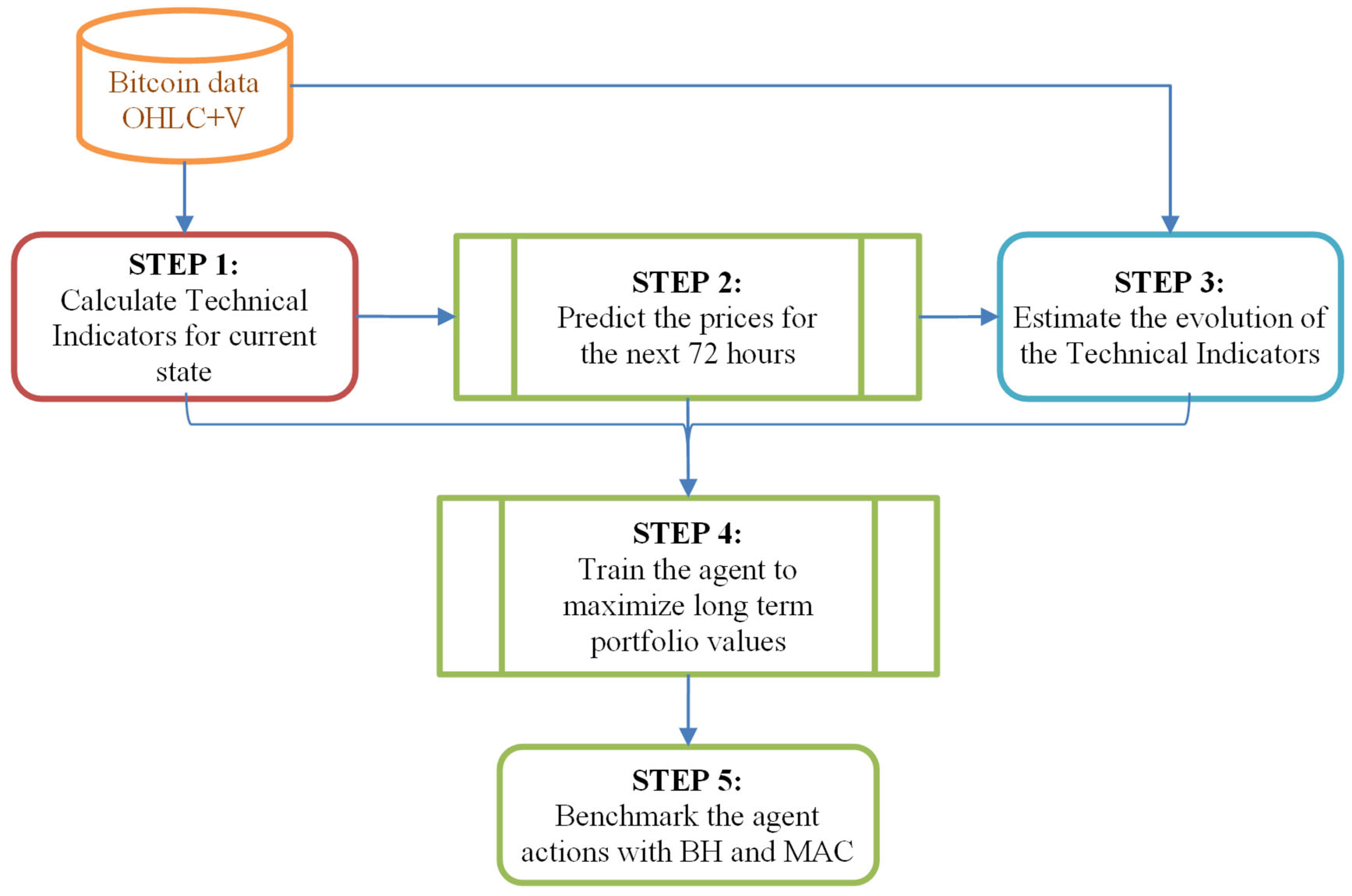
The proposed methodology aims to combine the supervised and reinforcement learning models to train an agent to perform trading actions on the bitcoin market using a complex environment consisting of bitcoin prices, volume, and technical indicators (trend, volume, volatility, and momentum) calculated for the current and future states. The methodology is composed of the following steps:

Step 1. Using the current values of the bitcoin prices and volume (OHLC+V), the following technical indicators are calculated for the current trading state: triple exponential moving average (TEMA), momentum, relative strength index (RSI), stochastic oscillator (STOK, STOD), rate of change (ROC), on-balance volume (OBV), Chaikin Money Flow (CMF), and Bollinger bands.

Step 2. The historical bitcoin prices are used to predict the bitcoin prices for the next 72 h using a univariate recurrent neural networks (RNNs) model. Two types of RNN models are trained and tested on the univariate model: LSTM and GRU.

Step 3. Based on the price predictions, the estimated values of the technical indicators are obtained and added to the state space to enhance the environment representation with the trend of the prices.

Step 4. The RL environment is defined in terms of action space, state space, and reward. Then, the RL agent is trained using four main RL models suitable for continuous spaces: proximal policy optimization (PPO), soft actor–critic (SAC), TD3, advantage actor–critic (A2C).

Step 5. The trading actions of the agent are compared with two common strategies: buy and hold (BH) and the moving average crossover (MAC).

These steps are depicted in Figure 1 and detailed in the following sections.

3.1. Calculating Technical Indicators for the Current State

The current values of bitcoin prices and volume (OHLC+V) are used to calculate the most relevant technical indicators in financial analysis. These indicators can be grouped as follows:

• Trend indicators provide the direction of market trends and include: EMA helps in identifying the trend direction over a period, indicating whether the market is moving upwards, downwards or sideways; TEMA is even more sensitive to recent price movements than EMA, aiming to reduce the lag that is often found in traditional moving averages. This increased sensitivity allows it to closely follow the price action, making it useful for identifying trends early. However, this sensitivity also means it may react more to short-term price volatility, potentially leading to false signals.
• Momentum indicators and oscillators measure the speed at which the price of bitcoin is changing. This category includes: RSI that indicates overbought or oversold conditions; momentum that measures the rate of change in price, which can signal the strength of a trend; stochastic oscillator that compares the closing price of bitcoin to its price range over a given time period. It consists of two main components: the %K line that is the main line of the stochastic oscillator and represents the current price level relative to the high–low range over a specific period. The %K line (STOK) is a measure of momentum, and it is calculated based on the closing prices over a given period. The %D line (STOD) is a moving average of the %K line and represents the “signal line” because it is used to generate buy or sell signals based on its crossover with the %K line. The %D line smooths out the %K values to help identify trends more clearly. Another momentum oscillator is price ROC that measures the percentage change in price between the current price and the price a certain number of periods ago (N). A positive ROC indicates upward momentum, while a negative ROC suggests downward momentum. High absolute values of ROC (either positive or negative) indicate strong trends, while values close to zero suggest a lack of trend or a market in consolidation.
• Volume indicators reflect the volume of trading and confirm trends or signal reversals. The most relevant indicators are OBV that uses volume flow to predict changes in stock price and CMF that combines the price and volume to show the buying and selling pressure over a period. The CMF value can range between −1 and 1; a positive CMF value suggests that buying pressure is dominant, indicating accumulation, and could be seen as a bullish sign, while a negative CMF value indicates that selling pressure is dominant, suggesting distribution that could be interpreted as a bearish sign.
• Volatility indicators express the rate at which the price increases or decreases, and the most relevant are Bollinger bands that show when bitcoin’s price is at an extreme. The middle band (BBMBand) indicates the intermediate-term trend, represented by the simple moving average (SMA); the upper band (BBUBand) shows the upper level of price volatility; and the lower band indicates the lower level of price volatility (BBLBand). These technical indicators are calculated using the equations provided in

  Table 1. Technical indicator equations.

  $\mathbf{Indicator} ({\mathit{T}\mathit{I}}^{\mathit{d}})$	Equation	No.
  ${\mathrm{E}\mathrm{M}\mathrm{A}}^d$	${EMA}^{d_0}={\displaystyle \frac{\sum _{d_{0\in N}}{CP}^{d_0}}{N}}$ ${EMA}_1^d={EMA}^{d_0}+{\displaystyle \frac{2}{N+1}}\times ({CP}^d-{EMA}^d)$	(1)
  ${\mathrm{T}\mathrm{E}\mathrm{M}\mathrm{A}}^d$	${TEMA}^d=3\times {EMA}_1^d-3\times {EMA}_2^d+{EMA}_3^d$ •  ${EMA}_2^t$ is the exponential moving average of ${EMA}_1$; • ${EMA}_3^t$ is the exponential moving average of ${EMA}_2$.	(2)
  ${\mathrm{R}\mathrm{S}\mathrm{I}}^d$	${RSI}^d={\displaystyle \frac{{\overline{CP}}_{+}}{{\overline{CP}}_{+}+{\overline{CP}}_{-}}}\times 100$ $\mathrm{w}\mathrm{h}\mathrm{e}\mathrm{r}\mathrm{e}: \left\{\begin{array}{c}{CP}_{+}^{∆d}=1\times ({CP}^d-{CP}^{d-1}), if {CP}^d-{CP}^{d-1}>0 \\ {CP}_{-}^{∆d}=-1\times ({CP}^d-{CP}^{d-1}), if C{P}^d-{CP}^{d-1}<0\end{array}\right.$	(3)
  ${Momentum}^d$	${Momentum}^d={CP}^d-{CP}^{d-1}$	(4)
  ${\mathrm{S}\mathrm{T}\mathrm{O}\mathrm{K}}^d, {\mathrm{S}\mathrm{T}\mathrm{O}\mathrm{D}}^d$	${\mathrm{S}\mathrm{T}\mathrm{O}\mathrm{K}}^d={\displaystyle \frac{{CP}^d-\underset{t\in T}{\min }{LP}^t}{\underset{t\in T}{\max }{HP}^t-\underset{t\in T}{\min }{LP}^t}}\times 100$ ${\mathrm{S}\mathrm{T}\mathrm{O}\mathrm{D}}^d={\displaystyle \frac{{\mathrm{S}\mathrm{T}\mathrm{O}\mathrm{K}}^{d-2}+{\mathrm{S}\mathrm{T}\mathrm{O}\mathrm{K}}^{d-1}+{\mathrm{S}\mathrm{T}\mathrm{O}\mathrm{K}}^d}{3}}$	(5)
  ${\mathrm{R}\mathrm{O}\mathrm{C}}^d$	${\mathrm{R}\mathrm{O}\mathrm{C}}^d={\displaystyle \frac{{CP}^d-{CP}^{d-N}}{{CP}^{d-N}}}\times 100$	(6)
  ${\mathrm{O}\mathrm{B}\mathrm{V}}^d$	${\mathrm{O}\mathrm{B}\mathrm{V}}^{\mathrm{d}}=\left\{\begin{array}{c}{OBV}^{d-1}+V^d, if {CP}^d>{CP}^{d-1}\\ {OBV}^{d-1}-V^d, if {CP}^d<{CP}^{d-1}\\ {OBV}^{d-1}, if{CP}^d={CP}^{d-1}\\ {\mathrm{V}}^{{\mathrm{d}}_0}, if d=d_0\end{array}\right.$	(7)
  ${\mathrm{C}\mathrm{M}\mathrm{F} }^d$	1. Calculate daily money flow multiplier (MFM): ${\mathrm{M}\mathrm{F}\mathrm{M} }^d={\displaystyle \frac{({CP}^d-{LP}^d)-({HP}^d-{CP}^d)}{{HP}^d-{LP}^d}}$ 2. Calculate the money flow volume (MFV): ${\mathrm{M}\mathrm{F}\mathrm{V} }^d={\mathrm{M}\mathrm{F}\mathrm{M} }^d\times V^d$ 3. Calculate the Chaikin Money Flow (CMF) for the specified number of periods (commonly 20 or 21 days): ${\mathrm{C}\mathrm{M}\mathrm{F} }^d={\displaystyle \frac{{\sum }_{d\in T}{\mathrm{M}\mathrm{F}\mathrm{V} }^d}{{\sum }_{d\in T}{\mathrm{V} }^d}}$	(8)
  ${\mathrm{B}\mathrm{B}\mathrm{M}\mathrm{B}\mathrm{a}\mathrm{n}\mathrm{d} }^d, {\mathrm{B}\mathrm{B}\mathrm{U}\mathrm{B}\mathrm{a}\mathrm{n}\mathrm{d} }^d,{\mathrm{B}\mathrm{B}\mathrm{L}\mathrm{B}\mathrm{a}\mathrm{n}\mathrm{d} }^d$	${\mathrm{B}\mathrm{B}\mathrm{M}\mathrm{B}\mathrm{a}\mathrm{n}\mathrm{d} }^d={SMA}_N={\displaystyle \frac{1}{N}}{\displaystyle \sum _{d=1}^N}{CP}^d$ ${\mathrm{B}\mathrm{B}\mathrm{U}\mathrm{B}\mathrm{a}\mathrm{n}\mathrm{d} }^d={\mathrm{B}\mathrm{B}\mathrm{M}\mathrm{B}\mathrm{a}\mathrm{n}\mathrm{d} }^d+2\sqrt{{\displaystyle \frac{1}{N-1}}}{\displaystyle \sum _{d=1}^N}{({CP}^d-{SMA}_N)}^2$ ${\mathrm{B}\mathrm{B}\mathrm{L}\mathrm{B}\mathrm{a}\mathrm{n}\mathrm{d} }^d={\mathrm{B}\mathrm{B}\mathrm{M}\mathrm{B}\mathrm{a}\mathrm{n}\mathrm{d} }^d-2\sqrt{{\displaystyle \frac{1}{N-1}}}{\displaystyle \sum _{d=1}^N}{({CP}^d-{SMA}_N)}^2$	(9)

  .

The output of this step is represented by the market vector $M^d$ that consists of current values of OHLC+V and technical indicators as in Equation (10):

$$M^d=[{OP}^d,{HP}^d,{LP}^d,{CP}^d,V^d,{TI}^d], \forall d\in T$$

(10)

where ${\mathit{T}\mathit{I}}^{\mathit{d}}=\left\{\begin{array}{c}{\mathit{E}\mathit{M}\mathit{A}}^{\mathit{d}},{\mathit{T}\mathit{E}\mathit{M}\mathit{A}}^{\mathit{d}},{\mathit{R}\mathit{S}\mathit{I}}^{\mathit{d}},{\mathit{M}\mathit{o}\mathit{m}\mathit{e}\mathit{n}\mathit{t}\mathit{u}\mathit{m}}^{\mathit{d}},{\mathit{S}\mathit{T}\mathit{O}\mathit{K}}^{\mathit{d}},{\mathit{S}\mathit{T}\mathit{O}\mathit{D}}^{\mathit{d}},{\mathit{R}\mathit{O}\mathit{C}}^{\mathit{d}},{\mathit{O}\mathit{B}\mathit{V}}^{\mathit{d}},\\ {\mathit{C}\mathit{M}\mathit{F}}^{\mathit{d}},{\mathit{B}\mathit{B}\mathit{M}\mathit{B}\mathit{a}\mathit{n}\mathit{d}}^{\mathit{d}},{\mathit{B}\mathit{B}\mathit{L}\mathit{B}\mathit{a}\mathit{n}\mathit{d}}^{\mathit{d}},{\mathit{B}\mathit{B}\mathit{U}\mathit{B}\mathit{a}\mathit{n}\mathit{d}}^{\mathit{d}}\end{array}\right\}$

3.2. Predict the Prices for the Next 72 h

To predict prices, two types of RNN models are used: LSTM and GRU. To predict the prices for the next days, both models are trained on a univariate model that consists only of the previous values of the bitcoin prices. Thus, the models are learning from a sequence of past observations to predict future values. The input data is organized into 24 h vectors, with each vector used to predict the following hour’s price. However, the objective extends beyond predicting just the immediate next hour’s price; it involves forecasting prices for the next 24 h up to 72 h. To achieve this, the model initially predicts the first future value, which is then incorporated back into the input sequence as part of a sliding window technique.

This process continues iteratively to forecast subsequent prices, generating a complete 24 h future price vector. This methodology is particularly tailored to scenarios like bitcoin price forecasting, where the prices for the current day (represented as a 24 h vector) are known, and the challenge lies in predicting the prices for the next days (another 72 h vector). Thus, predictions for earlier hours are used as inputs to forecast prices further ahead. Therefore, if the forecasting horizon extends to 48 or 72 h, this iterative prediction process is carried out 48 or 72 times. The accuracy of the first 24 h predictions is anchored on actual observed values and the immediate hourly forecasts, while the predictions for the subsequent 24 h are based solely on the forecasts from the previous day, making them less precise and more prone to errors.

Although the LSTM and GRU models output a single value at a time, the forecasting strategy enables the generation of a full 24 h prediction vector by sequentially updating the input vector with each new predicted value. This process involves two main phases: training the model on historical data and then employing it to make predictions. Through this approach, the model continuously refines its forecasts, utilizing the initial accurate predictions to inform the subsequent, thereby navigating through the 24 h prediction cycle.

The step-by-step process for predicting the hourly values of the next day (day d + 1) and the day after (d + 2), based on the hourly values of the current day (day d), is provided below:

Predicting day d + 1:

• First hour prediction uses the 24 hourly values from day $d$, denoted as $\left[{CP}^{d,1}, {CP}^{d,2},\dots ,{CP}^{d,23},{CP}^{d,24}\right]$, to predict the first hour of day d + 1, which is represented as ${\widehat{CP}}^{d+\mathrm{1,1}}$
• Second hour prediction incorporates the first hour prediction of day d + 1 along with the last 23 hourly values of day d to predict the second hour of day d + 1: $\left[{CP}^{d,2}, {CP}^{d,3},\dots ,{CP}^{d,24},{\widehat{CP}}^{d+\mathrm{1,1}}\right]\to {\widehat{CP}}^{d+\mathrm{1,2}}$
• Subsequent hour predictions continue the previous process iteratively, where each next hour prediction for day d + 1 uses the previous hour’s prediction as part of its input, until all 24 h of day d + 1 are forecasted. For example, the third hour prediction would be: $\left[{CP}^{d,3}, {CP}^{d,4},\dots ,{\widehat{CP}}^{d+\mathrm{1,1}},{\widehat{CP}}^{d+\mathrm{1,2}}\right]\to {\widehat{CP}}^{d+\mathrm{1,3}}$
• Repeat the pattern up to the 24th hour prediction to obtain the hourly predictions for the rest of the day: $\left[{CP}^{d,24},{\widehat{CP}}^{d+\mathrm{1,1}},\dots ,{\widehat{CP}}^{d+\mathrm{1,22}},{\widehat{CP}}^{d+\mathrm{1,23}}\right]\to {\widehat{CP}}^{d+\mathrm{1,24}}$

Predicting Day d + 2:

• First hour prediction of day d + 2 uses the 24 predicted hourly values from day d + 1 $\left[ {\widehat{CP}}^{d+\mathrm{1,1}},\dots ,{\widehat{CP}}^{d+\mathrm{1,22}},{\widehat{CP}}^{d+\mathrm{1,23}},{\widehat{CP}}^{d+\mathrm{1,24}}\right]$ as inputs to predict the first hour of day d + 2, represented as ${\widehat{CP}}^{d+\mathrm{2,1}}$
• Subsequent hour predictions for day d + 2. Similarly, for each subsequent hour of day d + 2, it uses the predictions from the previous hours of day d + 2 (starting from the predictions of day d + 1) as inputs. This iterative process continues until all 24 h of day d + 2 are forecasted, with the final prediction being $\left[{\widehat{CP}}^{d+\mathrm{1,24}}, {\widehat{CP}}^{d+\mathrm{2,1}},\dots ,{\widehat{CP}}^{d+\mathrm{2,22}},{\widehat{CP}}^{d+\mathrm{2,23}}\right]\to {\widehat{CP}}^{d+\mathrm{2,24}}$

Predicting Day d + 3:

The process applied for day d + 2 is repeated for day d + 3, and the hourly predictions are obtained for the entire day: $\left[{\widehat{CP}}^{d+\mathrm{3,1}}, \dots ,{\widehat{CP}}^{d+\mathrm{3,24}}\right]$. The output of this step is the predicted close price for the next 3 days ($\widehat{{CP}^d}$) represented as follows:

$${\widehat{CP}}^{d+\delta }=\left[{\widehat{CP}}^{d+\delta ,1},\dots ,{\widehat{CP}}^{d+\delta ,24}\right], \forall \delta \in [\mathrm{1,2},3]$$

(11)

To ensure methodological rigor, forecasts at time t are generated strictly using information available up to time t. The LSTM model is trained exclusively on the training set. During the testing period, forecasts are generated in a rolling approach: at each timestep, the input window consists only of historical observed prices up to that moment. No future realized prices are used in state construction, and predicted technical indicators are computed solely from forecasted prices rather than realized future prices. This chronological separation prevents any look-ahead bias or information leakage.

The forecasting model is designed based solely on historical bitcoin prices to serve as a short-term directional signal generator whose purpose is to provide forward-looking trend information to the reinforcement learning agent. Moreover, the state representation includes multiple volatility, momentum, and volume-based technical indicators derived from price, which implicitly capture important aspects of market dynamics such as volatility clustering and trend persistence. The focus of the proposed framework is therefore on evaluating the incremental value of forward-looking price structure within an RL environment rather than maximizing standalone predictive accuracy. Extending the framework to incorporate external variables constitutes a promising avenue for future work.

3.3. Estimate the Evolution of Technical Indicators

The predicted values of the prices are used to estimate the evolution of the technical indicators for the next days. Therefore, Equations (1)–(10) are used to calculate the indicators, replacing the actual close price with the predicted prices. As a result, the predicted values of the technical indicators (${\widehat{TI}}^{d+\delta }$) are obtained and added to the market vector $M^d$:

$$M^d\leftarrow \left[M^d,{\widehat{TI}}^{d+\delta }\right], \forall d\in T, \delta \in [\mathrm{1,2},3]$$

(12)

3.4. Train the Agent to Maximize Long-Term Portfolio Values

The trading model is formulated as a partially observed Markov decision process (POMDP), defining the following elements: state space, action space, and reward function. The state space is represented by the market vector and current state of the agent: current balance and number of shares held.

$${State}_s=[M_s^d, B_s,{BTC}_s]$$

(13)

where $s$ is the current step of the trading interval $T_s$.

The action space defines the trading actions of the agent as a combination of two variables: trade action (sell, buy, or hold) and amount. The action space is configured as $A=\left[{ActionType}_s, {Amount}_s\right]$ on a continuous interval bounded by [0, 0] and [3, 1] where:

$${ActionType}_s=\left\{\begin{array}{c}Buy, if{ActionType}_s<1 \\ Sell, if {ActionType}_s<2\\ Hold, otherwise\end{array}\right.$$

(14)

The amount is used to calculate the number of trading units ($u_s$), imposing balance and stock constraints. Therefore, if the amount exceeds the current balance, then the agent is limited to buying less than the indicated amount. If the sale amount is greater than the current shares held, the trading units are limited to the existing shares (15):

$$u_s=\left\{\begin{array}{c}{\displaystyle \frac{\min (B_s, {Amount}_s\times B_s) }{{CP}_s^d}}, if{ActionType}_s<1 \\ \min ({BTC}_s, {Amount}_s\times {BTC}_s) , if {ActionType}_s<2\\ 0, otherwise\end{array}\right.$$

(15)

After taking action, the net worth is calculated as in Equation (16), considering a transaction cost for trading ($\beta$). Usually, it is considered as a percentage of the trade value as a fee. This can vary depending on the action (buy/sell) and trading volume.

$${NetW}_s=B_s+{BTC}_s\times {CP}_s^d-\beta \times u_s\times {CP}_s^d$$

(16)

Reward is a scalar feedback signal of the trading actions that indicates how well the agent is doing at each step $s$, and it can be calculated as an immediate return as a difference between the current net worth obtained at step $s$ and the previous net worth at step $s-1$:

$${r_s={return}_s=NetW}_s-{NetW}_{s-1}$$

(17)

To encourage the agent to explore at the beginning of the training period, a delay factor is applied to adjust the reward. It is calculated as a ratio between the current step $s$ and the total number of steps ($T_s$):

$${r_s\leftarrow \rho r}_s$$

(18)

where $\rho ={\displaystyle \frac{s}{T_s}}$—is the delay factor.

Also, a more realistic approach in the reward function is to penalize drawdowns and adjust for portfolio volatility, aiming for a balance between high returns and sustainable risk management. Implementing these adjustments provides a more balanced and robust approach to training of the RL agent.

The drawdown penalty factor ($\phi$) penalizes the agent for significant drops in portfolio value, encouraging strategies that minimize large losses. Initially, it has a small value to ensure that the agent is not overly penalized for normal market fluctuations. It is incrementally increased until the agent starts to avoid risky actions that lead to large drawdowns without being too conservative. As a starting point, a value between 0.1 and 0.3 is selected. The reward is updated using Equation (19):

$$r_s\leftarrow {(1+\phi )\times r}_s, if r_s<0$$

(19)

The volatility penalty factor ($\vartheta$) penalizes the agent for maintaining a portfolio with high volatility, promoting stability in the portfolio’s return. Similar to the drawdown penalty, initially, a lower value is selected between 0.01 and 0.05, and it is adjusted based on the observed behavior of the agent. If portfolio volatility is high without commensurate returns, then the value is increased up to 0.1. Portfolio volatility is typically calculated using the standard deviation of returns over a certain period. To include the volatility penalty factor, the reward at each step is updated as follows:

$$r_s\leftarrow r_s-\vartheta \sqrt{{\displaystyle \frac{1}{s-1}}\sum _{i=1}^s{\left({return}_s-\overline{return}\right)}^2}$$

(20)

where $\overline{return}$ is the average return over the previous $s$ steps, and $\sqrt{{\displaystyle \frac{1}{s-1}}{\sum }_{i=1}^s{\left({return}_s-\overline{return}\right)}^2}$ represents the portfolio volatility over the current number of steps.

The drawdown and volatility penalty factors are initialized within commonly used ranges (e.g., 0.1–0.3 for drawdown and 0.01–0.05 for volatility) for financial reward shaping and then iteratively calibrated to balance risk control and learning stability. Instead of optimizing these values for maximum reward, which may lead to overfitting, the penalties are adjusted based on the observed training dynamics, ensuring that the agent avoided large portfolio losses while maintaining sufficient exploration. This procedure follows standard practice in RL-based trading systems, where risk-aware reward shaping is typically guided by empirical behavior rather than fixed theoretical constants.

Cumulative reward with discounting. Emphasizing long-term rewards rather than immediate profit can be an effective strategy for encouraging the agent to develop strategies that are sustainable over time rather than optimizing for short-term gains. Thus, the agent learns to navigate through volatility and make decisions that are beneficial in the long run. One standard method to prioritize long-term rewards is to use a discounted reward approach, where future rewards are considered but discounted at each timestep. Thus, the main goal of the agent is to maximize the total future rewards using the following equation:

$$R_s=\sum _{k=0}^{T_s}{\gamma }^k{r}_{s+k+1}$$

(21)

where $\gamma$ is the discount factor, and $\gamma \in [0,1]$ and $k$ represents the future steps. A value close to 0 leads to a “myopic” or short-term reward, and a value close to 1 leads to a far-sighted or long-term reward. Setting a value around 0.9 encourages the agent to consider the long-term consequences of its actions, which is particularly relevant in bitcoin trading where short-term gains might be outweighed by long-term profitability and risk management.

For reproducibility, the coefficients used in the reward formulation are explicitly defined as follows. The drawdown penalty factor $\varphi$, introduced in Equation (19), and the volatility penalty factor $\vartheta$, introduced in Equation (20), are positive scalar constants that control the relative weight of drawdown and volatility penalization with respect to the net worth change term. The discount factor $\gamma \in [0,1]$, defined in Equation (21), determines the relative importance of future rewards in the cumulative objective function. In all reported experiments, the coefficients were fixed at: $\varphi =0.2$, $\vartheta =0.05$, and $\gamma =0.05$. These parameters remained constant during training and evaluation and are not dynamically updated within episodes.

The reward formulation can be interpreted as a mean–variance objective with drawdown regularization, which is conceptually related to utility functions incorporating risk aversion and downside risk penalties in modern portfolio theory.

RL training models. For training the agent in an RL environment, especially in complex tasks like bitcoin trading, several algorithms can be considered. Each algorithm comes with its own strengths and is suited to different types of problems. In the current approach, several models are selected and compared based on the following considerations:

• PPO belongs to the family of policy gradient methods. It addresses some of the complexities and challenges associated with training policy-based RL algorithms, particularly those related to choosing an appropriate step size for updating policies.
• SAC is an off-policy actor–critic method that optimizes a stochastic policy in an off-policy way, aiming for both efficiency and stability.
• TD3 improves upon the deep deterministic policy gradient (DDPG) algorithm by addressing function approximation errors through techniques like clipped double-Q learning and delayed policy updates.
• A2C is simpler to implement and versatile, suitable for both discrete and continuous action spaces. In the simulation section, these models are used to train the agent, and their results are compared.

The experimental results reported in the simulations are obtained using a hybrid continuous formulation. Specifically, the action vector consists of two components: (i) a categorical trading decision (buy, sell, or hold), internally encoded as a continuous variable and discretized into three regions; and (ii) a continuous trade amount in the interval [0, 1], representing the proportion of available balance (for buy) or holdings (for sell) to transact. Therefore, PPO, SAC, TD3, and A2C are implemented in a continuous action setting, where the policy outputs both the action type and trade size jointly. This formulation allows flexible position sizing while preserving interpretable trading decisions.

3.5. Benchmark the Agent Actions with BH and MAC

Benchmarking the RL trading agent against well-known strategies is crucial to evaluate its performance and practical value. Two common benchmarks in trading activities are the buy-and-hold (BH) strategy and the moving average crossover (MAC) strategy. BH represents the canonical passive exposure baseline for bitcoin, while MAC represents a standard rule-based active strategy driven solely by past prices. These two baselines are commonly used in RL-based trading studies because they provide interpretable lower-bound performance references and help quantify the economic value of adaptive trading relative to (i) market exposure and (ii) simple technical heuristics. BH strategy involves buying bitcoin at the beginning of the evaluation period and holding it until the end. It is a strategy that bets on the long-term appreciation of the asset. MAC strategy involves two moving averages of the price: a short-term moving average and a long-term moving average. A buy signal is generated when the short-term moving average crosses above the long-term moving average, and a sell signal is generated when the opposite crossover occurs. To prove its performance, the proposed RL trading agent should consistently outperform these benchmarks; therefore, in the simulation section, multiple episodes of testing are performed, and the profits obtained by the agent are calculated and compared with BH and MAC profits. The profit rate (PR) is calculated for each method using Equation (22):

$$PR={\displaystyle \frac{{NetW}_{T_s}-B_0}{B_0}}$$

(22)

where ${NetW}_{T_s}$ is the final portfolio value obtained at the end of the episode, and $B_0$ is the initial investment.

Also, risk-adjusted returns are evaluated by calculating the risk (volatility) of these strategies. Thus, if the RL trading agent achieves slightly lower returns than a benchmark method but with significantly lower volatility, it might still be considered more successful. A key indicator that is used to evaluate the performance of an investment relative to its risk is Sharpe ratio (SR) calculated as in Equation (23):

$$SR={\displaystyle \frac{{ER}_{BTC}-{ER}_f}{{\sigma }_{BTC}}}$$

(23)

where: ${ER}_{BTC}$ is the expected return of the bitcoin portfolio, ${ER}_f$ is the risk-free rate of return, and ${\sigma }_{BTC}$ is the standard deviation of the portfolio’s excess return, which represents the risk of the portfolio.

For a bitcoin trading agent operating within an RL framework, determining an appropriate risk-free rate (${ER}_f$) poses a unique challenge. Unlike traditional portfolio management scenarios, where ${ER}_f$ is often derived from the yield of a government bond or similar low-risk investment, the context of bitcoin trading necessitates a different approach, primarily due to the high volatility and the absence of a direct equivalent to a risk-free asset in cryptocurrency markets. Thus, a risk-free rate can be considered as a fixed, low risk-free rate that reflects the opportunity cost of not investing in a minimal risk asset outside the cryptocurrency market. This could be based on short-term government bond yields from a stable economy, acknowledging that while not directly applicable to crypto, it provides a baseline for comparison. Another approach, especially relevant in highly speculative or volatile markets like bitcoin, is to assume a zero risk-free rate. Using a zero risk-free rate focuses the analysis purely on the excess returns generated by the trading strategy over the assumed baseline of holding cash (or cash equivalents) with no interest.

The SR helps investors understand how much excess return they are receiving for the extra volatility that they endure for holding a riskier asset. A higher Sharpe ratio indicates a more attractive risk-adjusted return.

4. Simulations

4.1. Data Description

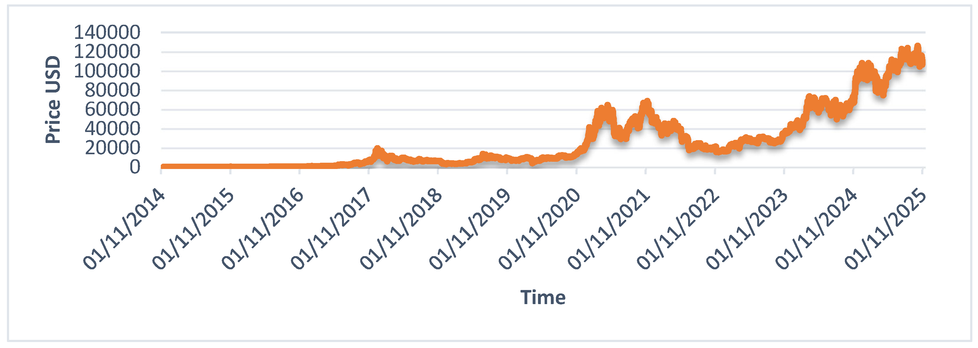
The dataset consists of Bitcoin prices and volume recorded hourly between November 2014 and October 2025, including almost 96,091 hourly records (https://github.com/simonavoprea/bitcoin_trading, accessed on 31 October 2025). The dataset is split into a training set with records before the 31 March 2023 and a test set with records between the 1 April 2023 and the 30 October 2025. The training set is used for training the models (both supervised and reinforcement learning), and the test set is used for evaluation. The split is carried out based on the evolution of bitcoin prices (Figure 2); the training set captures the spikes and gaps that have some similarities with the test set. The selected 2014–2025 interval already encompasses multiple pronounced market regimes, including sharp bull–bear transitions, volatility spikes, and macro-driven structural shifts, providing a sufficiently rich and representative environment for evaluating the proposed hybrid forecasting–RL framework.

To eliminate any possibility of implicit look-ahead bias, the entire modeling pipeline is implemented under a strict chronological separation between forecasting and RL stages. First, the LSTM model is trained exclusively on the training dataset (November 2014–March 2023) using only historical observations available within that interval. Once trained, the LSTM parameters are frozen and not updated during RL training or evaluation.

During the testing period (April 2023–October 2025), rolling forecasts are generated sequentially in real time: at each timestep $t$, the 72 h price predictions are computed using only observed prices up to time $t$. The predicted values are then used to calculate forward-looking technical indicators, which are appended to the state vector available to the RL agent at that same timestep.

RL training episodes are constructed strictly within the training interval, while evaluation episodes are sampled exclusively from the test interval. At no point are future realized prices, technical indicators, or portfolio outcomes used in constructing the state representation for decision-making at time $t$.

4.2. Hyperparameters of the Models

The hyperparameters of the prediction models (LSTM and GRU) are tuned using learning and validation curves. The following hyperparameters are tuned: number of units (neurons), number of hidden layers, learning rate, dropout rate, optimizer and activation function. Hyperparameter tuning for the RL mode involved systematically adjusting the model’s hyperparameters to improve its performance in the environment, measured by the cumulative reward. To evaluate the values of the hyperparameters, the average cumulative reward achieved by the model in the environment is plotted over a set number of consistent episodes. Then, the values that maximize the cumulative reward are selected. The following hyperparameters are tuned: discount factor ($\gamma$) determines the present value of future rewards, and a gamma close to 1 (between 0.9 and 0.99) means that future rewards are almost as important as immediate rewards; learning rate; and entropy coefficient, which encourages exploration by the agent during the learning process. For the policy of the agent, the MLP policy is selected which is a standard choice trading, where the observation space and action space are fully numerical. MLP networks are capable of capturing complex relationships between the state (market indicators) and the optimal actions (buy, sell, hold). The optimal values of the hyperparameters are in

Table 2. The optimal values of the hyperparameters.

Model	Hyperparameter	Optimal Value
Supervised learning LSTM, GRU	Number of units (neurons)	[128, 64]
	Number of hidden layers	2
	Learning rate	0.001
	Dropout rate	0.2
	Optimizer	Adam
	Activation function	Rectified linear unit (relu)
Reinforcement learning PPO, A2C, SAC, TD3	Discount factor	0.95
	Learning rate	0.0001
	Entropy coefficient	0.2
	Policy	MLPPolicy

.

The models are implemented in Python 3.13, using TensorFlow and Keras for LSTM and Stable Baseline 3 and OpenAI Gym for the RL models. The trading environment is defined using the action space, observation (state) space, and reward function described in Section 3.4. The episodes are randomly selected from the datasets, and each episode consists of 180 days’ hourly records. The 180-day episodes are selected because this window is long enough to capture complete bitcoin market regimes (trend reversals, volatility clusters, and structural breaks) while still allowing a large number of independent samples for training and evaluation. Shorter windows fail to represent full market dynamics, whereas much longer windows reduce statistical diversity. Episodes are randomly sampled from the test set to expose the agent to heterogeneous market conditions and to ensure statistically robust performance estimates across multiple independent scenarios rather than a single contiguous time interval. The initial investment or balance is set to 100,000 USD.

Experiments were conducted using fixed random seeds (seed = 42 for TensorFlow, NumPy, PyTorch, and Stable Baselines3). Each experiment was repeated across five independent seeds, and the results were averaged. Average training time per RL model was approximately 40 min on NVIDIA RTX 3090 GPU while LSTM and GRU training required less than 15 min.

4.3. Predicting the Close Price for the Next 3 Days; Evaluation of the LSTM and GRU Models

The prediction of the bitcoin prices using LSTM and GRU is obtained based on the historical sequences of the dataset. To compare the models in terms of performance metrics, the results are presented in

Table 3. Forecasting results for the entire testing period corresponding to one-step-ahead hourly forecasts.

Prediction Model	MAE	RMSE	R2
LSTM	185	331	0.99
GRU	192	349	0.98

.

Since LSTM demonstrated superior performance compared to GRU, it is employed to generate bitcoin price forecasts for the next 72 h, which are incorporated as additional features in the state space of the RL environment.

The high coefficient of determination (R² ≈ 0.99) reported in Table 3 corresponds to one-step-ahead hourly forecasts. Such elevated values are consistent with the strong short-term autocorrelation observed in high-frequency bitcoin price series, where consecutive hourly prices exhibit limited absolute variation relative to overall price level.

For longer recursive horizons, forecasting accuracy gradually deteriorates due to error propagation inherent in multi-step iterative forecasting. Specifically, when predictions are recursively fed back as inputs, small estimation errors accumulate over time, leading to increasing deviation from realized prices. Thus, MAE increases from 185 USD for one-step forecasts to approximately 420 USD on the 72 h horizon. Similarly, RMSE rises from 331 USD to 631 USD, while R² decreases from 0.99 to approximately 0.92.

This gradual performance decay is expected in highly volatile and partially stochastic markets such as bitcoin, particularly when using recursive multi-step forecasting. Even at the 72 h horizon, the model preserves substantial explanatory power (R² > 0.90), indicating that the predicted price trajectories retain meaningful directional information, which is subsequently exploited by the reinforcement learning agent.

Although forecasting accuracy declines at longer recursive horizons due to error accumulation, the RL agent does not treat predicted prices as deterministic future outcomes. The forecasted prices and their derived technical indicators are incorporated as auxiliary features within a multidimensional state representation that also includes current indicators, volume dynamics, and portfolio state variables.

During training, the agent optimizes realized portfolio reward based on actual market movements rather than forecast accuracy. If longer-horizon predictions become noisy, their contribution to decision-making is implicitly adjusted through policy learning, as actions leading to poor realized returns are penalized by the reward function. Moreover, the inclusion of drawdown and volatility penalties further reduces sensitivity to overconfident responses to inaccurate long-horizon signals.

Therefore, the recursive forecasting error does not propagate directly into portfolio loss but is filtered through the RL optimization process, which selects actions based on realized outcomes. The forecasting component should thus be interpreted as a directional signal enhancer rather than a precise multi-step price estimator.

4.4. Training the Agent; Evaluation of the RL Models

To prepare the environment of the RL models, the state space is built from the current prices and volume (OHLC+V) and the current values of the technical indicators [12,40]. For reproducibility, the drawdown and volatility penalty factors used in the reward function were calibrated during the initial training runs. The penalties were initialized at the lower bound of the recommended ranges (φ = 0.1 for drawdown, and ϑ = 0.02 for volatility) and increased in small fixed increments (Δφ = 0.02, Δϑ = 0.01) only when the agent displayed repeated large drawdowns or excessive portfolio variance. Adjustment stopped once reward evolution curves and portfolio behavior became stable, resulting in final penalty values of φ = 0.2 and ϑ = 0.05, which were consistently used in all experiments. This simple rule-based procedure prevents overfitting while ensuring stable and risk-aware learning behavior. 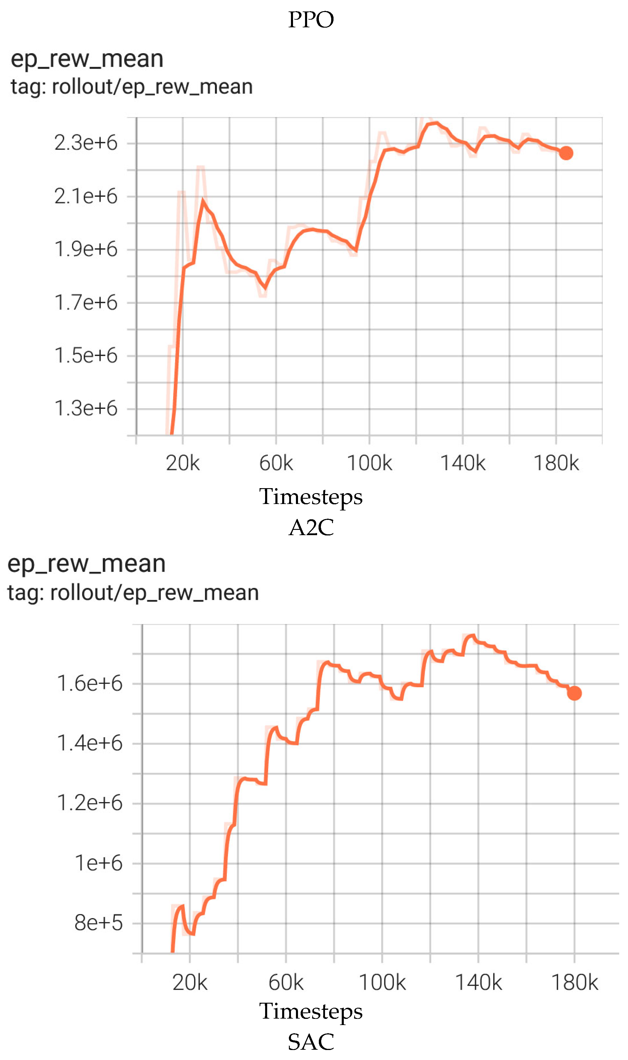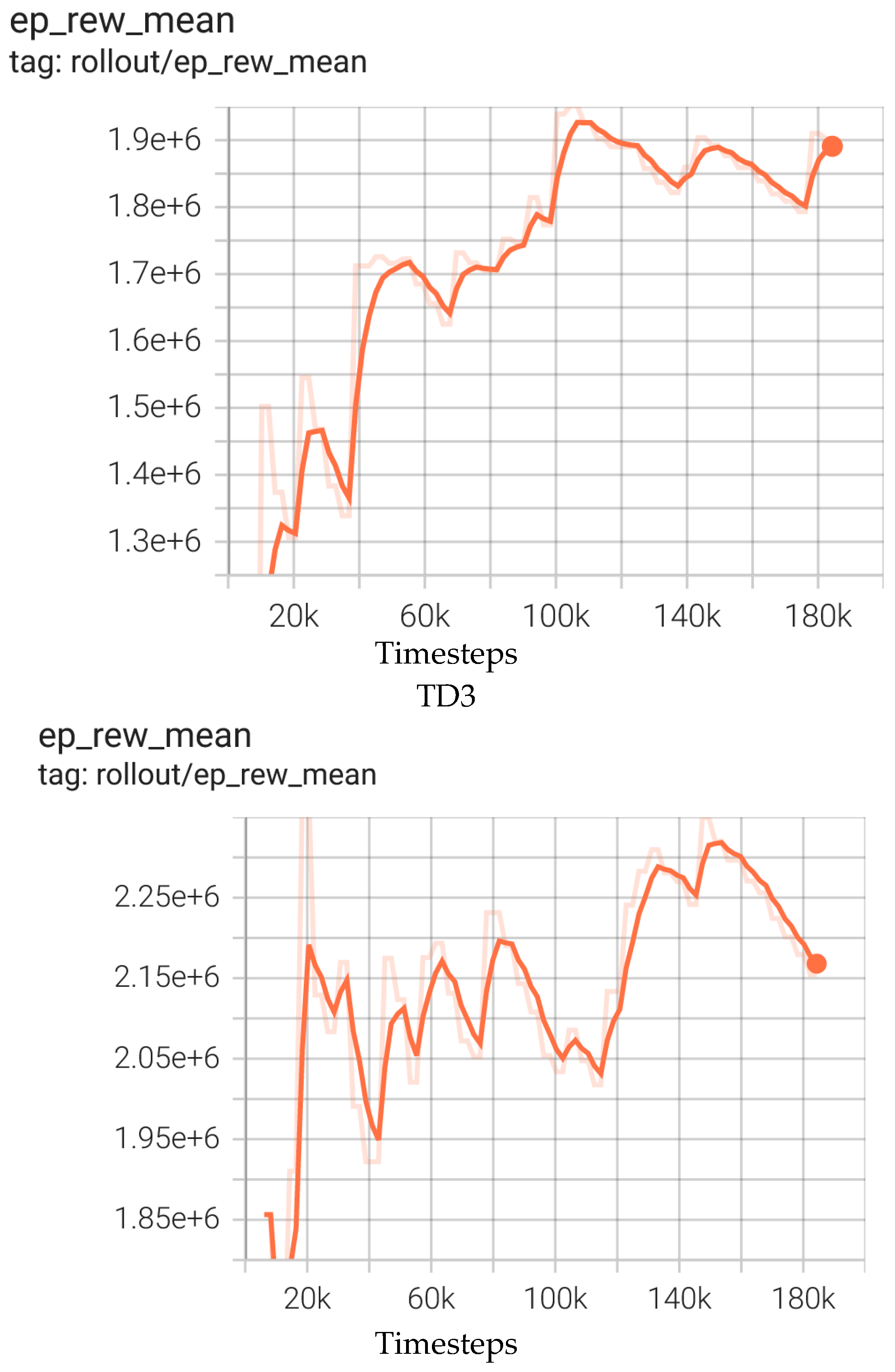As a baseline, the RL agent is trained and tested using this state for comparison reasons with the enhanced variant of the state’s space that includes the estimations of the technical indicators. After forecasting the next 72 h of the prices, the estimations of the technical indicators are obtained using Equations (1)–(10) and added to the observation space as in Equation (14). Thus, the enhanced variant of the state space is obtained, and the agent is trained in this environment. For reproducibility, the drawdown and volatility penalty factors used in the reward function were calibrated during the initial training runs. For training the agent, the following RL models are used and compared: PPO, A2C, SAC, and TD3. The evaluation was performed on 30 episodes of 180 days during the testing set, and the mean reward is obtained for each model. PPO obtains a mean reward of $2.34\times {10}^6$, A2C reward mean is $1.68\times {10}^6$, SAC obtains a mean reward of $1.95\times {10}^6$, and TD3’s reward mean is $2.31\times {10}^6$ (as in Figure 3).

The reward in Figure 3 represents the cumulative portfolio return accumulated over each 180-day episode, where a reward equal to the change in net worth is added at every hourly timestep. The cumulative reward per episode reaches magnitudes on the order of 10⁶ due to the aggregation of hourly net worth changes over 180-day intervals with an initial capital of 100,000 USD. While the absolute reward scale may appear large, it does not affect algorithm comparison, since all RL models are trained under an identical reward formulation and scaling.

The absolute scale of the reward allows a consistent comparison of training stability and convergence across RL algorithms, all of which use the same reward formulation. Although TD3 obtained a high mean reward per episode, its reward curve shows multiple fluctuations and decreases to $2.17\times {10}^6$ at the end of the timesteps. Therefore, the PPO model is selected for training the RL agent. To evaluate the trading actions, the RL agent is tested on multiple episodes on the test set. 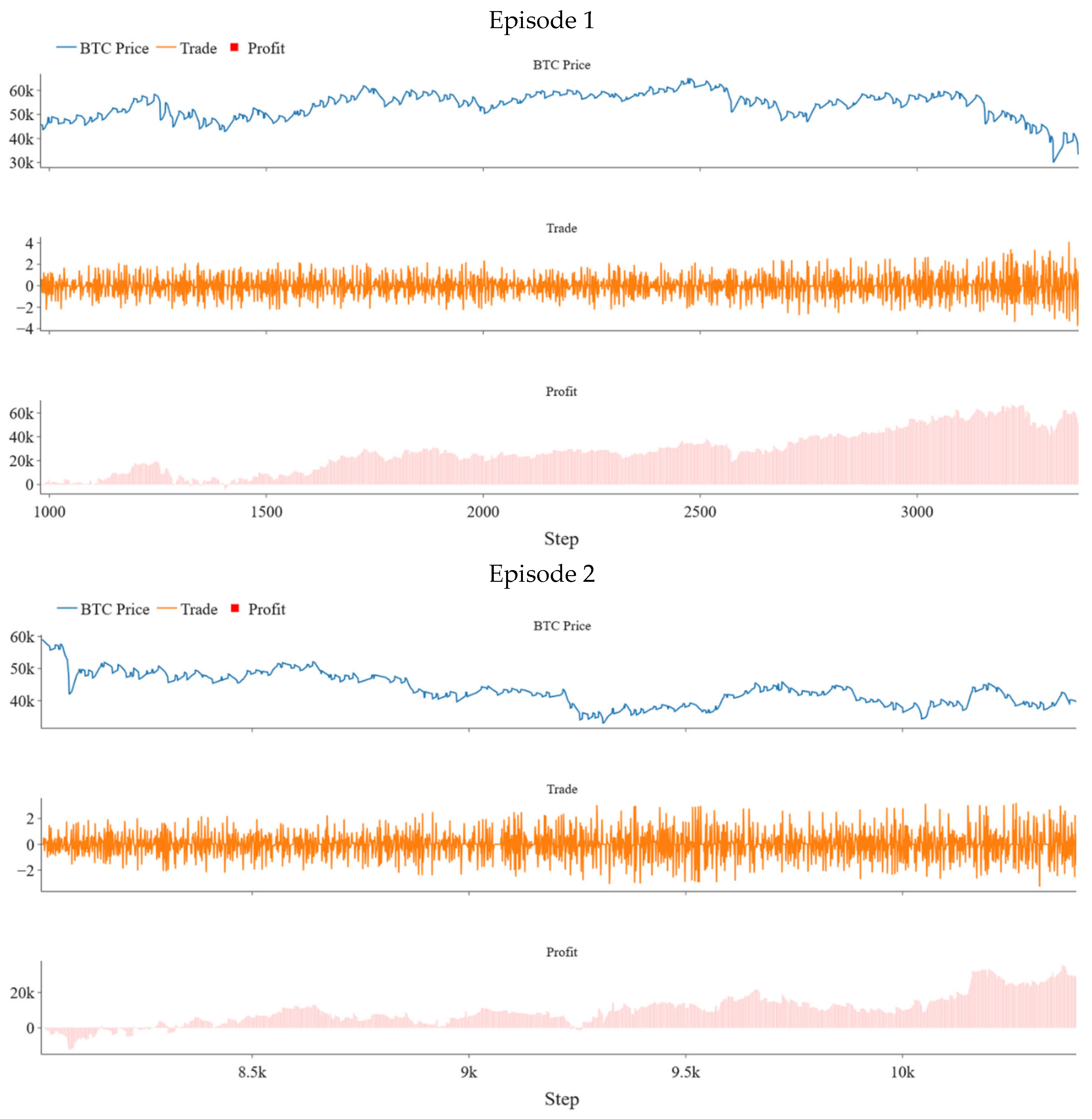Figure 4 illustrates two representative episodes to provide a qualitative view of the agent’s trading behavior and equity evolution. These examples are not intended to reflect overall performance. The quantitative evaluation is based on 100 randomized out-of-sample episodes, and the aggregated results presented in

Table 4. Comparison between the proposed agent, baseline, and the benchmarking strategies for 100 episodes.

Strategy	Profit (USD)	Profit Ratio (%)		Sharpe Ratio
		Mean	Standard Deviation	Mean	Standard Deviation
BH	17,000	17	10.5	0.93	0.28
MAC	12,000	12	12.3	0.45	0.35
Baseline	27,000	27	9.2	1.17	0.24
Agent	32,000	32	7.5	1.34	0.19

capture performance across the full test period. Thus, the evaluation ensures that the conclusions are not dependent on any single market interval.

The first sub-plot depicts the evolution of the bitcoin prices as a reference of the trend. The second sub-plot presents the size and direction of trades (buying or selling) indicating the magnitude and type of each trade. As can be observed, the agent is actively trading throughout the period, with varying trade sizes. The third sub-plot reflects the profit or loss for each step. The profit is mostly above the zero line, indicating that the agent is making a profit over many of the steps, although there are periods of loss as well, especially at the beginning of the episodes. Even if the prices registered a significant decrease towards the end of the interval, the agent managed to keep and even increase the profit, especially during Episode 1.

To verify scale invariance, we conducted additional experiments using normalized rewards, obtained by dividing each step reward by the initial portfolio value. The relative ranking of algorithms (PPO outperforming A2C, SAC, and TD3) remained unchanged, and performance differences were statistically consistent. This confirms that algorithm comparison is not driven by reward magnitude but by policy learning dynamics.

To assess the agent’s performance, the profit, PR, and SR are calculated using Equations (22) and (23). For interpretability in financial terms, we report PR and SR as primary evaluation metrics, which are independent of cumulative reward scale. The results are compared with the baseline values and the benchmarking strategies: BH and MAC. These strategies represent the two most widely used and conceptually distinct baselines in RL-based trading research. BH reflects the passive market exposure benchmark, while MAC represents a classical technical-indicator-driven active strategy. Performance metrics are averaged across 100 independent test episodes, which provides a robust estimate of expected performance and naturally captures variability across market conditions. This multi-episode evaluation is standard in RL studies and serves the role of statistical validation without requiring additional hypothesis-testing procedures. The results are shown in Table 4 (average values).

The absolute profit reported in USD in Table 4 is provided as a descriptive indicator of the magnitude of returns. All strategies operate under the same initial capital (100,000 USD) and identical trading constraints, so position sizing is fixed across methods. For meaningful comparison, the analysis relies primarily on the PR, which normalizes returns by initial investment, and the SR, which incorporates portfolio volatility. These two metrics provide the risk-adjusted and position-size-independent basis for evaluating and comparing strategy performance. We computed standard deviations across the 100 independent test episodes to assess variability. The proposed agent achieved a PR of 32% (std = 7.5%) and an SR of 1.34 (std = 0.19), indicating stable performance across heterogeneous market conditions. A paired t-test comparing the agent and the BH strategy confirms that the improvement in PR is statistically significant at the 1% level (p < 0.01). Therefore, the reported outperformance is not driven by isolated favorable episodes but reflects consistent behavior.

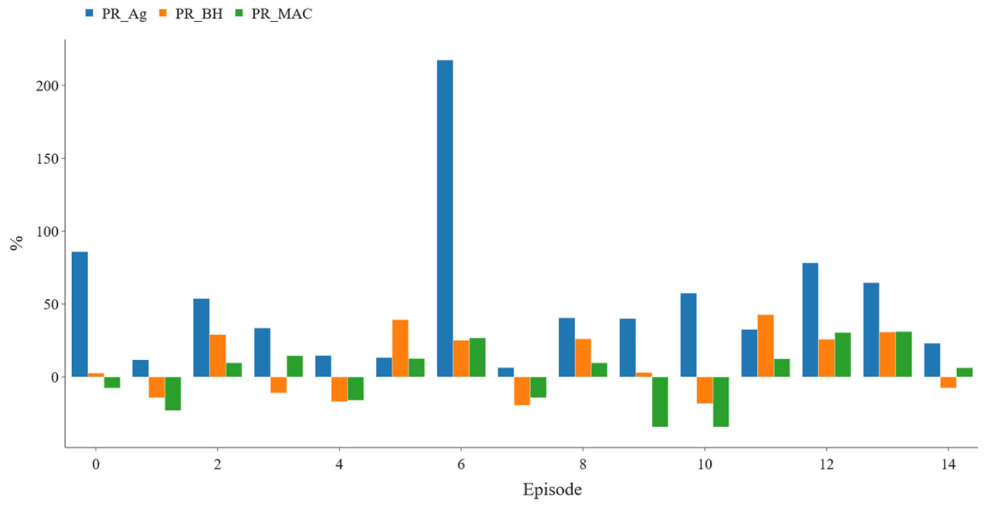
In Figure 5, the PR obtained by the agent on 15 consecutive episodes is compared to the PR obtained by the BH and MAC strategies. RL agent’s PR proves to be higher than the two strategies across episodes. It has episodes of outperformance, notably in Episode 1, 6, and 10. The RL agent significantly outperforms the other strategies, indicating that the agent’s strategy aligns exceptionally well with market movements.

The BH strategy appears to have a relatively consistent performance, with lower variance compared to the RL agent. Although its PR is positive in most of the episodes, it does not reach the level of the RL agent’s performance. The MAC strategy generally underperforms compared to the other two strategies, with many episodes showing very low or negative profit.

4.5. Robustness and Comparative Analysis

While Section 4.4 presents the primary evaluation results of the proposed framework, additional robustness and comparative analyses are conducted to further validate the stability, generalization capacity, and marginal contribution of each methodological component.

To assess robustness, we conducted a grid-based sensitivity analysis over drawdown penalty φ ∈ {0.1, 0.2, 0.3} and volatility penalty ϑ ∈ {0.02, 0.05, 0.1}. Results indicate that the proposed agent consistently outperforms baseline strategies across all configurations. Performance variation remained within ±3% for PR and ±0.08 for SR, demonstrating that the proposed reward formulation is not critically dependent on a single parameter configuration.

Beyond performance robustness, varying the drawdown (φ) and volatility (ϑ) penalties influences the qualitative behavior of the trading policy. Increasing the drawdown penalty encourages more conservative position sizing during adverse market movements, leading to earlier exposure reduction and lower maximum drawdown. Similarly, higher volatility penalties reduce portfolio variance by discouraging rapid position changes and excessive leverage, which results in smoother equity curves and lower turnover.

Conversely, lower penalty values allow the agent to assume more aggressive positions, increasing potential profitability but also exposing the portfolio to higher short-term fluctuations. Across the tested grid, we observe a trade-off between raw PR and risk stabilization: moderate penalty values (φ = 0.2, ϑ = 0.05) provide the most balanced risk-return profile, maximizing SR without substantially sacrificing profitability. It confirms that the reward formulation acts as a controllable risk-preference mechanism rather than an arbitrary adjustment, allowing the framework to be tuned according to different risk tolerance levels.

4.5.1. Ablation Study

To isolate the marginal contribution of the two key methodological components of (i) forecasted technical indicators and (ii) risk-aware reward shaping, we conducted a structured ablation study. The objective was to determine whether the observed performance improvements arise primarily from predictive state enrichment, reward regularization, or their interaction. Four experimental configurations were evaluated in Table 5 under identical training and testing conditions:

-

Baseline RL—standard state representation using only current technical indicators and a reward based solely on immediate net worth changes.

-

Baseline + forecasted indicators—state augmented with 72 h forecasted technical indicators but without drawdown or volatility penalties.

-

Baseline + risk-aware reward—original state representation but including drawdown and volatility penalties in the reward function.

-

Full model (proposed framework)—combined use of forecasted indicators and risk-aware reward shaping.

Table 5. Comparison between the baseline model and variants using the ablation study.

Variant	PR	SR
Baseline	27	1.17
+Forecast	29	1.22
+Risk penalties	30	1.26
Full model	32	1.34

Table 5. Comparison between the baseline model and variants using the ablation study.

Variant	PR	SR
Baseline	27	1.17
+Forecast	29	1.22
+Risk penalties	30	1.26
Full model	32	1.34

All configurations were evaluated over 100 independent 180-day test episodes. The inclusion of forecasted indicators alone improves the PR relative to the baseline, indicating that forward-looking technical signals provide useful directional information. Introducing risk-aware reward shaping without forecast augmentation also enhances performance, particularly in terms of SR, confirming that volatility and drawdown penalties promote more stable portfolio trajectories.

The full model achieves the highest PR and SR. This suggests a complementary effect: predictive state enrichment improves decision quality, while risk-aware reward shaping regularizes behavior and prevents excessive volatility. Therefore, the joint configuration produces a more balanced and robust trading strategy than either modification alone. These findings demonstrate that the proposed hybrid architecture is not driven by a single enhancement but by the interaction between predictive signals and risk-aware optimization.

Also, it provides insight into the impact of predictive uncertainty on the trading policy. The “Baseline” configuration represents the agent operating without any forward-looking signal, while the “Baseline + Forecast” variant reflects the incremental contribution of the 72 h predictive component. The moderate performance improvement (PR increase from 27% to 29%) indicates that the predictive signal enhances decision-making but does not dominate the policy.

Consequently, if forecasting errors increase at longer horizons, the agent’s behavior does not collapse but gradually converges toward the baseline configuration. This suggests that the RL framework integrates forecasted indicators as probabilistic directional cues rather than deterministic future prices, thereby maintaining robustness under predictive uncertainty.

4.5.2. Sensitivity to Transaction Costs

The current implementation assumes a proportional transaction cost of β = 0.1% per trade, consistent with average exchange fees for liquid cryptocurrency markets. However, to assess the sensitivity of the proposed framework to higher execution costs and partially capture the effect of additional market frictions (e.g., bid–ask spread and slippage), we conducted a robustness analysis under elevated transaction cost assumptions. Thus, the agent was re-evaluated under β ∈ {0.2%, 0.5%}, while maintaining identical training and evaluation procedures. These higher values approximate the combined exchange fees and implicit execution costs in less favorable liquidity conditions. The results indicate that as expected, profitability decreases monotonically with increasing transaction costs. Under β = 0.2%, the average PR declines from 32% to 29%, and under β = 0.5%, it decreases to 24%. Nevertheless, the proposed agent continues to outperform both BH and MAC strategies. These findings suggest that the proposed hybrid forecasting–RL framework is not critically dependent on optimistic transaction cost assumptions and retains performance robustness under more conservative execution scenarios.

4.5.3. Regime-Based Performance Analysis

Bitcoin markets are known to exhibit structural regimes characterized by persistent upward trends (bull phases), downward corrections (bear phases), and periods of heightened volatility. To evaluate the robustness of the proposed framework across heterogeneous market conditions, we conducted a regime-stratified performance analysis.

Market regimes were identified using a simple and transparent classification rule based on rolling 30-day returns and volatility:

-

Bull regime: rolling 30-day return > +10%;

-

Bear regime: rolling 30-day return < −10%;

-

High-volatility regime: rolling 30-day return within ±10% but with realized volatility in the top quartile of the full sample.

Each 180-day test episode was categorized according to the dominant regime within the interval, and performance metrics were computed separately for each group.

Results in

Table 6. Regime-specific performance of agent, BH and MAC strategies.

Regime	Agent		BH		MAC
	PR%	SR	PR%	SR	PR%	SR
Bull	38	1.57	25	1.20	20	1.04
Bear	12	0.93	−8	−0.33	−11	−0.51
High volatility	24	1.24	10	0.67	8	0.42

indicate that the proposed RL agent maintains positive profitability across all regimes. In bull markets, the agent captures upward momentum and achieves its highest average PR. In bear markets, although absolute returns decline as expected in downward-trending environments, the agent significantly reduces losses compared to the BH strategy due to its ability to adjust exposure dynamically. During high-volatility sideways periods, the risk-aware reward formulation contributes to superior SR relative to BH and MAC strategies.

This regime-stratified analysis demonstrates that the hybrid forecasting–RL framework generalizes across structurally different market environments and does not rely exclusively on favorable bull-market conditions for its performance.

4.5.4. Computational Considerations

The proposed framework involves two main computational components: (i) the LSTM forecasting module and (ii) RL policy training. As previously reported, model training is performed offline. LSTM/GRU training required less than 15 min, while RL training per model required approximately 40 min on an NVIDIA RTX 3090 GPU.

The deployment does not require retraining at every timestep. Once trained, both the LSTM and RL policy operate in inference mode. Generating a 72 h recursive forecast involves 72 sequential forward passes of a lightweight univariate LSTM network, resulting in negligible computational cost (on the order of milliseconds). Similarly, RL decision-making consists of a single forward pass through the trained policy network, which is computationally low-cost.

Therefore, while the training phase involves moderate computational effort, real-time deployment is computationally efficient and suitable for hourly decision intervals. The framework does not require continuous retraining and can be updated periodically (e.g., daily or weekly) depending on market dynamics.

5. Conclusions

The paper presents a hybrid training approach that merges supervised and reinforcement learning to develop an RL agent to execute strategic trades in the bitcoin marketplace. The trading environment is augmented with a set of technical indicators, including TEMA, RSI, OBV, ROC, momentum, Chaikin Money Flow, and Bollinger bands, which are applied not only to current bitcoin prices but also to forecasts extending 72 h ahead. These forecasts are obtained using an LSTM univariate model. The predicted prices are then utilized to calculate future values of technical indicators, thereby enriching the trading environment. A reward function is defined for training the RL agent, taking into account long-term performance by incorporating penalties for drawdowns and volatility, thereby modelling the bitcoin market’s dynamics more realistic. The RL agent’s strategy is tested over a series of randomly chosen episodes, each spanning 180 days of hourly data from 2023 and 2024. The agent’s profitability, PR, and SR are assessed and benchmarked against conventional strategies such as BH and MAC. The RL agent outperforms the comparative strategies, delivering an average PR of 32% and an SR of 1.34. This is compared to the BH strategy, which achieves a PR of 17% and an SR of 0.93, and the MAC strategy, which obtained a PR of 12% and an SR of 0.45. While BH and MAC provide informative classical benchmarks, a comprehensive contemporary RL comparison would include additional learned baselines such as DQN/A2C/PPO trained with a standard reward (e.g., immediate net worth change) and without forecast augmentation, as well as implementations from public trading–RL frameworks (e.g., FinRL-style baselines). Because the main objective of this study is to isolate and validate the effect of forecast-enriched state design and risk-aware reward shaping, we focus the experimental section on these reference strategies and on controlled variants of the proposed environment. Extending the benchmark suite with additional RL and non-RL baselines is an important direction for future work and would further strengthen external comparability.

In the present study, transaction costs are incorporated directly into the execution of each trading action. Specifically, whenever the agent buys or sells, the trade value is adjusted using a proportional trading fee β = 0.1%, which reduces the available balance for buy orders and the received proceeds for sell orders. The updated balance and position size, already adjusted for this fee, are then passed into the next state of the RL environment. While transaction costs are explicitly modelled, other important market frictions are not included in the current implementation. These include bid–ask spreads, liquidity and depth constraints, slippage, and additional position-size limitations beyond those imposed by the agent’s current balance and holdings. Since our objective was to isolate the effect of the hybrid forecasting–RL framework under controlled conditions, microstructure-level frictions were left for future extensions. Nevertheless, we acknowledge that incorporating spread-, slippage- and liquidity-sensitive execution models would increase realism and may influence the agent’s performance, and we identify this as an important direction for further research.