Preference-Aligned Ride-Sharing Repositioning via a Two-Stage Bilevel RLHF Framework

Abstract

Vehicle repositioning is essential for improving efficiency and service quality in ride-sharing platforms, yet existing approaches typically optimize proxy rewards that fail to reflect human-centered preferences such as wait time, service coverage, and unnecessary empty travel. We propose the first two-stage Bilevel Reinforcement Learning (RL) from Human Feedback (RLHF) framework for preference-aligned vehicle repositioning. In Stage 1, a value-based Deep Q-Network (DQN)-RLHF warm start learns an initial preference-aligned reward model and stable reference policy, mitigating the reward-model drift and cold-start instability that arise when applying on-policy RLHF directly. In Stage 2, a Kullback–Leibler (KL)-regularized Proximal Policy Optimization (PPO)-RLHF algorithm, equipped with action masking, behavioral-cloning anchoring, and alternating forward–reverse KL, fine-tunes the repositioning policy using either Large Language Model (LLM)-generated or rubric-based preference labels. We develop and compare two coordination schemes, pure alternating (PPO-Alternating) and k-step alternating (PPO-k-step), demonstrating that both yield consistent improvements across all tested arrival scales. Empirically, our framework reduces wait time and empty-mile ratio while improving served rate, without inducing trade-offs or reducing platform profit. These results show that human preference alignment can be stably and effectively incorporated into large-scale ride-sharing repositioning.

1. Introduction

1.1. Motivation

Vehicle repositioning is essential for improving reliability and efficiency in Mobility-on-Demand (MoD) systems, as it enables platforms to reduce wait times, increase service availability, and respond to spatial demand variations [1,2]. In ride-sharing settings, effective repositioning must balance several human-centric performance metrics, such as wait time, served rate, and empty-mile ratio (abbreviated as ‘empty ratio’ or ‘empty’ in some figures or tables), which naturally interact and often conflict.

Prior research has explored algorithms for improving matching efficiency or dispatching decisions [3,4], and Reinforcement Learning (RL)-based repositioning methods have shown promise [5,6,7]. However, these approaches rely on manually designed proxy rewards that do not explicitly reflect human-preferred trade-offs. As a result, policies may optimize operational metrics while neglecting factors that matter to riders or operators. Previous work such as [8] has also applied RL to urban transportation systems to reduce congestion and travel time. They develop multi-agent Deep Reinforcement Learning controllers for urban traffic lights that coordinate signal phases across multiple intersections. Their Proximal Policy Optimization and Deep Q-Network-based models significantly reduce travel time and traffic congestion compared to traditional methods, which indicates that RL can directly optimize congestion in urban mobility systems. In this work, we focus instead on ride-sharing repositioning, where the platform must jointly balance waiting time, served rate, and empty miles under stochastic demand.

Meanwhile, Reinforcement Learning from Human Feedback (RLHF) has emerged as a powerful framework for aligning policies with preference data, but it has seen limited application in transportation domains. Integrating preference learning into repositioning requires both (i) learning a reward model that captures human-valued outcomes, and (ii) optimizing a repositioning policy using that learned reward while ensuring stable behavior in a many-to-many movement environment.

Motivated by these needs, we develop a two-stage bilevel RLHF framework for preference-aligned ride-sharing repositioning. A value-based Deep Q-Network (DQN)-RLHF warm start produces initial preference-aligned reward weights and a reasonable starting policy, and a Kullback–Leibler (KL)-regularized Proximal Policy Optimization (PPO)-RLHF stage refines the policy using either Large Language Model (LLM)-assisted or rubric-based preference labels. With action masking and First-In-First-Out (FIFO)-based matching incorporated into training, the proposed approach enables repositioning decisions that jointly improve wait time, served rate, and empty-mile ratio across a range of arrival scales. Beyond these general sectors, our proposed method is motivated to address the under-emphasis on human-centered experiences in prior repositioning research. Additionally, the proposed method applies an on-policy RLHF framework in a many-to-many movement environment while avoiding high variance and unstable training via a two-stage design under KL-regularized PPO with action masking.

1.2. Related Work

1.2.1. Reinforcement Learning and Optimization for Ride-Sharing Repositioning

Vehicle repositioning is central to improving the performance of Mobility-on-Demand (MoD) systems, enabling platforms to reduce wait times, increase service coverage, and better utilize limited fleets. Classical studies demonstrate the value of optimized vehicle movement and demand-aware routing [1,2].

Matching-based dispatch algorithms such as the Hungarian assignment [3] and online bipartite matching [4] efficiently pair vehicles and passengers, but they operate in a one-to-one setting and do not directly address the many-to-many movement decisions required for repositioning. Rebalancing strategies using zone-based heuristics or predictive control further improve availability [9,10], and large-scale industrial systems often rely on combinatorial dispatching [11].

Reinforcement Learning (RL) methods have been increasingly applied to repositioning [5,6,7,12], typically optimizing handcrafted proxy rewards designed to approximate service quality or operational efficiency. However, these proxy rewards often fail to represent nuanced human-centric trade-offs, such as balancing wait time against empty miles or preserving fairness across regions. To our knowledge, no prior work has incorporated explicit human preference alignment into the repositioning objective.

1.2.2. Reinforcement Learning from Human Feedback (RLHF)

RLHF has emerged as a powerful framework for aligning decision-making policies with human judgments. Standard RLHF pipelines learn a reward model from pairwise preference data, often using Bradley–Terry formulations [13], and then optimize a policy using RL methods such as PPO [14]. More recently, bi-level RLHF frameworks such as [15,16,17] explicitly alternate between reward-model updates and policy optimization, supporting both round-based and k-step update schedules. While these methods establish general-purpose RLHF templates, prior work has not explored their application to ride-sharing or vehicle repositioning, where decisions must be made on spatial networks, under many-to-many movement constraints, and with operational baselines such as FIFO.

1.2.3. Stabilization Techniques for Policy Optimization

Stable RL optimization is essential in structured decision-making problems. Action masking has been shown to improve feasibility and reduce undesirable behavior by restricting actions to contextually valid subsets [18]. Behavioral cloning (BC) and imitation-based regularization [19,20] provide additional stability by anchoring learning toward a reference behavior, particularly valuable during early training.

Proximal Policy Optimization (PPO) [14] has become the standard RL algorithm within RLHF due to its clipped objective and KL-based trust region control. KL regularization helps keep the updated policy close to a reference [21], and alternating between reverse and forward KL can further stabilize training [22,23]. Adaptive KL coefficients and temperature scaling [24] adjust regularization strength dynamically, mitigating instability in optimization.

Value-based warm starts, such as those provided by Double DQN [25], are known to reduce overestimation and improve sample efficiency. However, their role as initialization mechanisms in RLHF pipelines, particularly for repositioning, has received limited attention. Our work introduces a two-stage RLHF formulation where a DQN-RLHF warm start produces preference-aligned reward estimates and a stable reference policy, which are then refined by PPO-RLHF under masking and imitation-based stabilizers.

1.3. Contributions

This paper introduces the first preference-aligned vehicle repositioning framework based on a two-stage bilevel RLHF design. Our contributions are summarized as follows:

• Two-stage RLHF framework for ride-sharing repositioning. We propose a value-based DQN-RLHF warm start followed by an on-policy PPO-RLHF refinement stage integrating action masking and imitation anchoring to coordinate multiple vehicles, prevent over-clustering and ensure operationally feasible repositioning in a many-to-many ride-sharing environment. This design stabilizes preference learning and provides a reliable reference policy for subsequent optimization.
• Preference-aligned reward learning for repositioning. Human preferences, obtained via LLM-assisted or rubric-based labeling, are incorporated through a Bradley–Terry model, enabling repositioning decisions that reflect wait time, served rate, and empty-mile trade-offs rather than handcrafted proxy rewards.
• Consistent empirical gains across demand regimes. Across multiple arrival scales, our two PPO-RLHF policies (PPO-Alternating and PPO-k-step) yield consistent improvements in wait time, served rate, and empty-mile ratio without sacrificing platform performance when comparing to no-reposition and classical baseline (heuristic).

1.4. Organization

The remainder of this paper is organized as follows: Section 2 presents the problem formulation, including the environment setup, the FleetEnvironment, and the optimization objective. Section 3 describes the proposed two-stage bilevel RLHF framework, detailing the action masking strategy, preference fitting, regularization components, and the two coordination schemes. Section 4 outlines the simulation setup and reports the evaluation results, including ablation studies demonstrating the effectiveness of the proposed method. Section 5 concludes the paper and discusses potential directions for future research. Additional notation and supplementary figures are provided in the Appendix A, Appendix B, Appendix C, Appendix D and Appendix E.

2. Problem Formulation

We consider a ride-sharing system consisting of an order matcher that assigns passenger requests to vehicles and a repositioning policy that moves idle vehicles across a spatial grid. The interaction between these components determines service quality, vehicle efficiency, and overall system performance. Figure 1 illustrates the grid environment and an example trajectory that includes repositioning, pickup, and drop-off movement. Shaded blocks represent demand zones 1–3. Zones 1–3 are three example zones in order to illustrate repositioning and pickup/dropoff trips. Zone 1 is a 4 × 4 central block in the middle of the grid. Zones 2 and 3 are two smaller 2 × 2 regions located near opposite corners of the grid. The simulator itself generates requests on the full grid according to the Poisson–diurnal model without any special zone-specific differences. The dashed blue line indicates a repositioning move, and the red arrows show one served request (pickup and drop-off).

The simulation takes place on a $10\times 10$ grid G with time step $\Delta t=30$ s, cell size $0.5$ km, and horizon $T=1200$ steps (10 h). A fleet of $N=90$ single-capacity vehicles operates on this grid. Passenger requests arrive according to a Poisson process whose rate is modulated by a diurnal function, creating realistic temporal demand variation. To simulate different request levels, we use a diurnal function with two peaks around the morning and evening periods and relatively lower intensity in the middle of the day. Internally, the simulator scales the Poisson arrival rate up during the peaks and down during off-peak times, so that the instantaneous request intensity varies between roughly 0.6 and 2.2 on a normalized scale, with the busiest times being a bit more than twice as busy as the quietest period. The spatial distribution of demand is homogeneous across the grid. At each step t, the total number of new requests is drawn from the time-varying Poisson process, and each request independently samples an origin and a destination uniformly over the 10 × 10 grid. Arrival-scale parameters $\alpha \in [0.60,1.00]$ represent different load regimes and are used throughout the evaluation.

With $\left|G\right|=100$ cells, the vehicle density is

$${\rho }_{\mathrm{veh}}={\displaystyle \frac{N}{\left|G\right|}}\approx 0.9\mathrm{vehicles}/\mathrm{cell}\approx 3.6{\mathrm{vehicles}/\mathrm{km}}^2$$

(1)

representing a medium-load operating environment. When scaling the grid size (e.g., $10\times 10\to 20\times 20$), the fleet size is increased proportionally (e.g., $90\to 360$) in order to maintain the same density. Conversely, varying the density at a fixed grid size (e.g., $N:90\to 110$ on $10\times 10$) enables controlled experiments on operational capacity. The 0.5 km cell resolution and $25{\mathrm{km}}^2$ area approximate a small urban district. These default settings provide a reproducible medium-scale environment; scalability experiments vary the grid size and fleet density accordingly.

Each request is defined by its origin, destination, and arrival time. Newly generated requests enter a queue, and a FIFO–nearest matching rule assigns requests to feasible idle vehicles subject to both a maximum-wait threshold and a radius bound $r_j$. This rule reflects operational practice and avoids over-concentration of vehicles. Ablation experiments additionally evaluate alternative matching rules, including greedy insertion and random assignment.

Vehicles move on the grid using Manhattan distance [26]. Idle vehicles follow repositioning decisions from a learned policy, while vehicles with assigned passengers follow precomputed shortest paths for pickup and drop-off. At each step, the environment updates vehicle states, request queues, travel statistics, and performance metrics such as served rate, wait time, cruising time, and empty miles.

The system is modeled as a discounted episodic Markov Decision Process (MDP)

$$\mathcal{M}=(\mathcal{S},\mathcal{A},P,R,\gamma ),\gamma =0.99$$

(2)

In the ride-sharing repositioning problem, relocation decisions have long-term effects on vehicle availability and request coverage over time steps. A high discount factor makes the agent care about rewards many steps in the future, so it values the long-term effects of repositioning vehicles toward demand instead of only improving the immediate match. A state $s_t$ encodes (i) the spatial distribution and occupancy of vehicles, (ii) request queues across grid cells, (iii) time-of-day indicators, and (iv) a short-term pickup heatmap summarizing recent demand patterns. Each idle vehicle selects an action

$$a_t\in \{\mathrm{stay},\mathrm{N},\mathrm{S},\mathrm{W},\mathrm{E}\}$$

(3)

corresponding to dwelling or moving one cell north, south, west, or east. State transitions $P(s_{t+1}\mid s_t,a_t)$ result from the combined effects of vehicle motion, order assignment, and service completion.

The goal is to learn a repositioning policy that reflects human preferences over key service metrics rather than relying on handcrafted proxy rewards. Each trajectory $\tau$ is summarized by a feature vector

$${\varphi }_{\tau }=\{\mathrm{served}\mathrm{rate}, \mathrm{empty}\text{-}\mathrm{mile}\mathrm{ratio}, \mathrm{cruising}\mathrm{hours}, \mathrm{movement}\mathrm{cost}\}$$

(4)

The served rate is defined as the fraction of requests that are successfully served, the empty-mile ratio is the fraction of vehicle-miles traveled without passengers over the total vehicle-miles, the cruising hours measure the total time that vehicles spend idling while waiting for requests, and the movement cost aggregates the distance traveled by repositioning moves. Together, these four features summarize each trajectory in terms of service quality (served rate), passenger experience (cruising hours), and operational efficiency (empty-mile ratio and movement cost).

Pairwise preference comparisons over trajectories are fitted using a Bradley–Terry model, producing preference weights w that define a shaped per-step reward,

$$\begin{array}{ccc}\hfill r_t& =\hfill & {\mathbf{w}}^{\top }{\mathit{\varphi }}_t\hfill \\ \hfill & =\hfill & w_{\mathrm{served}}{\Delta }_{\mathrm{served}}-w_{\mathrm{empty}}{\Delta }_{\mathrm{empty}}-w_{\mathrm{cruising}}{\Delta }_{\mathrm{cruising}}-w_{\mathrm{move}}·{\mathrm{move}}_t.\hfill \end{array}$$

(5)

The scalars $w_{\mathrm{served}}$, $w_{\mathrm{empty}}$, $w_{\mathrm{cruising}}$, and $w_{\mathrm{move}}$ are the preference weights learned by the Bradley–Terry model. Intuitively, a larger $w_{\mathrm{served}}$ increases the value of trajectories that serve more requests, whereas larger $w_{\mathrm{empty}}$ and $w_{\mathrm{cruising}}$ penalize unnecessary empty travel and long cruising time. The reward term $w_{\mathrm{move}}$ plays the role of an operational regularizer on repositioning distance. At each upper-level update, the preference model produces an updated per-step reward $r_t$. This provides a connection between human preferences at the trajectory level and the per-step reward used by the lower-level RL algorithms.

The resulting trajectory-level reward is

$$R_{\theta }\left(\tau \right)=\sum _{t=0}^{T-1}{r}_t$$

(6)

The preference-aligned policy optimization problem is

$$\underset{\pi }{max}{\mathbb{E}}_{\tau \sim \pi }\left[R_{\theta }\left(\tau \right)\right]$$

(7)

where the expectation is taken over trajectories generated by policy $\pi$ under the environment dynamics. To promote stable learning, particularly during early training when the reward model is still being refined, we incorporate an imitation regularizer that encourages $\pi$ to remain close to a reference policy ${\pi }_{\mathrm{ref}}$ obtained from the Stage-1 warm start.

During the PPO-RLHF stage, policy optimization proceeds through a KL-regularized objective of the form

$$\underset{\theta }{max}{\mathbb{E}}_{\tau \sim {\pi }_{\theta }}\left[\sum _{t=0}^{T-1}{r}_t-\beta \mathrm{KL}\left({\pi }_{\theta }(·|s_t)\parallel {\pi }_{\mathrm{ref}}(·|s_t)\right)\right]$$

(8)

where $\beta$ is an adaptive coefficient automatically tuned to maintain a target KL divergence between the current policy and the reference policy, following standard practice in RLHF [14,21]. This KL term prevents rapid policy drift, stabilizes optimization, and ensures that preference-updated rewards do not induce abrupt, undesirable behavior.

Our simulation relies on the following modeling assumptions:

1.

Customer requests follow a Poisson process with a fixed diurnal function on a 10 × 10 grid.

2.

Travel time between two cells is proportional to the Manhattan distance [26] with a constant speed (no congestion model).

3.

All vehicles are homogeneous and centrally controlled. Drivers always follow the repositioning decisions.

4.

The preference model evaluates policies only through three metrics: wait time, served rate, and empty-mile ratio.

Let $N_{\mathrm{req}}$ be the total number of generated requests in a period and $N_{\mathrm{served}}$ be the number of requests that are successfully served. Served rate (dimensionless) is defined as

$$\mathrm{served}\mathrm{rate}={\displaystyle \frac{N_{\mathrm{served}}}{N_{\mathrm{req}}}}$$

(9)

Wait time (minutes) is defined as

$$\mathrm{wait}\mathrm{time}=\mathrm{wait}\_\mathrm{pickup}\_\mathrm{steps}\times {\displaystyle \frac{\Delta t}{60}}$$

(10)

where we record the number of simulation steps between request creation and pickup for each served request with a step length of $\Delta t=30$ s.

Empty-mile ratio (dimensionless) is defined as

$$\mathrm{empty}\text{-}\mathrm{mile}\mathrm{ratio}={\displaystyle \frac{D_{\mathrm{empty}}}{\mathrm{VMT}}}$$

(11)

In Equation (11), VMT = $D_{\mathrm{empty}}+D_{\mathrm{loaded}}$, where $D_{\mathrm{empty}}$ and $D_{\mathrm{loaded}}$ denote the total empty and loaded distances traveled by all vehicles in an episode.

3. Two-Stage Bilevel RLHF Framework

This section presents the proposed two-stage bilevel RLHF framework for preference-aligned vehicle repositioning. The framework consists of a value-based warm start stage based on Double DQN and a policy-gradient stage based on PPO with KL regularization. Both stages interact with a learned preference-based reward model, which is updated from pairwise trajectory comparisons.

The two stages are tightly coupled rather than independent. Stage 1 learns an initial preference-aligned reward model and a stable reference policy ${\pi }_{\mathrm{ref}}$ using a Double DQN RLHF procedure with FIFO-nearest matching. Stage 2 starts from ${\pi }_{\mathrm{ref}}$ and the learned reward model from Stage 1 in the initial round. Later on, it uses the reward model from the previous round and fine-tunes a stochastic policy $\pi$ via PPO-RLHF with action masking and KL regularization. Overall, Stage 1 shapes the reward model and provides a safe starting point, while Stage 2 performs policy improvement under KL regularization starting from the initial model learned by Stage 1. Two coordination schemes are considered: a purely alternating outer loop and a k-step style alternating loop.

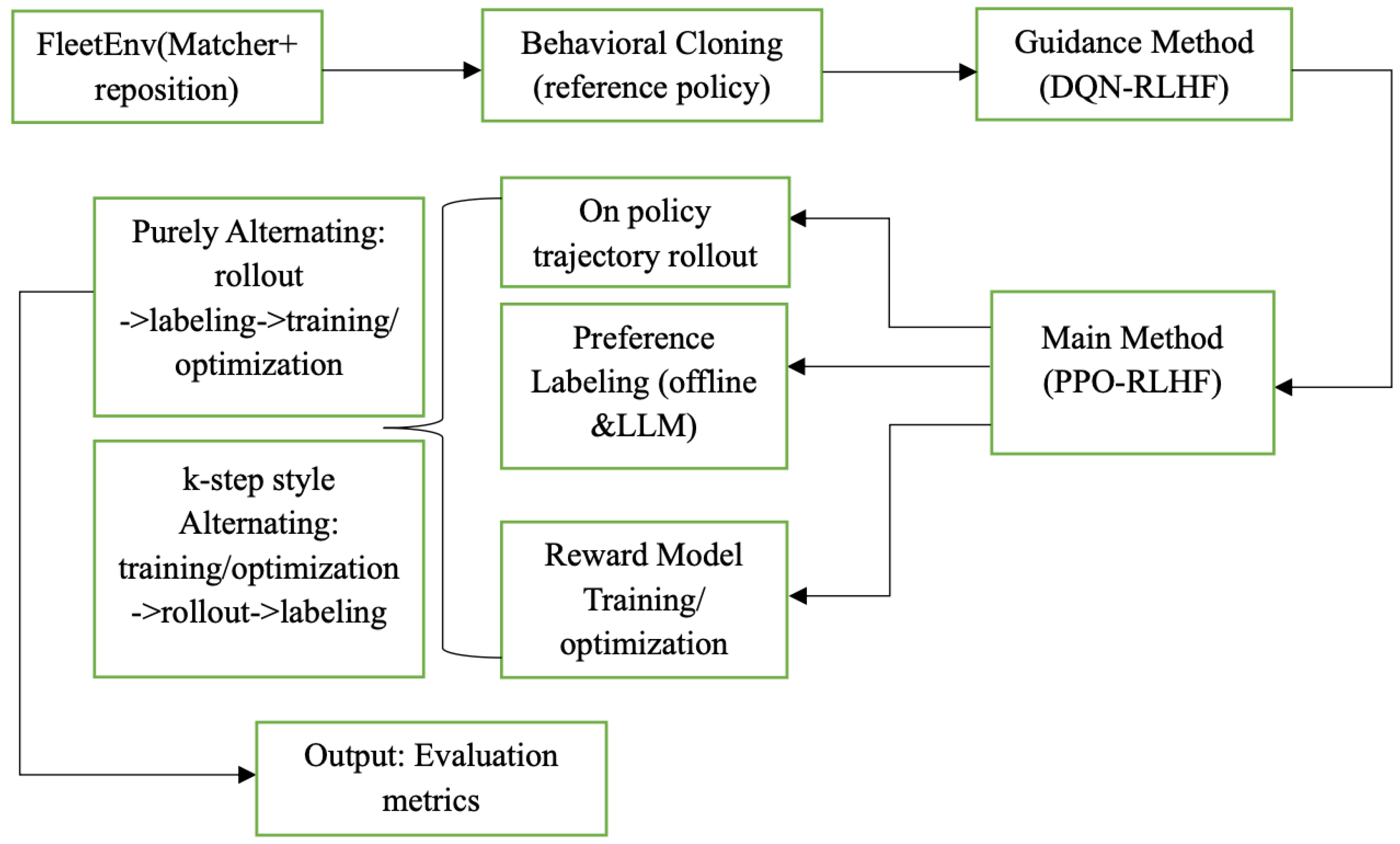
Figure 2 summarizes the two-stage bilevel RLHF framework. Requests generated by FleetEnv (Matcher + reposition) are used to train a Behavioral Cloning policy at first and then the guidance method (DQN-RLHF). After obtaining the initial weight and reward function, the main method (PPO-RLHF) produces on-policy trajectories. These trajectory preferences are labeled through a combination of an offline rubric and LLM assistance. Then, they will enter the lower-level loop to complete reward model training and optimization. The main method follows either a purely alternating scheme (rollout → labeling → training/optimization) or a k-step alternating scheme (training/optimization → rollout → labeling).

3.1. Action Masking

At each decision step, an idle vehicle at grid location $\mathrm{current}=(x_{\mathrm{cur}},y_{\mathrm{cur}})$ may move toward a target location $(x_{\mathrm{tar}},y_{\mathrm{tar}})$ or remain in place. The Manhattan distance between these locations is

$$\mathrm{dist}(\mathrm{current}, \mathrm{target})=|x_{\mathrm{cur}}-x_{\mathrm{tar}}|+|y_{\mathrm{cur}}-y_{\mathrm{tar}}|$$

(12)

Two distance thresholds are used to restrict the available actions: $R_{\mathrm{stop}}$ and $R_{\mathrm{go}}$. For a state s and corresponding distance $\mathrm{dist}\left(s\right)$ to the nearest relevant target (for example, a demand hotspot or previously chosen goal), the feasible action set $\mathcal{A}\left(s\right)$ is defined as

$$\mathcal{A}\left(s\right)=\left\{\begin{array}{cc}\left\{\mathrm{st}\right\},\hfill & \mathrm{dist}\left(s\right)\le R_{\mathrm{stop}},\hfill \\ \{\mathrm{st},1\text{-}\mathrm{step}\},\hfill & R_{\mathrm{stop}}<\mathrm{dist}\left(s\right)\le R_{\mathrm{go}},\hfill \\ \left\{\mathrm{st}\right\}\cup \mathcal{T}\left(s\right),\hfill & \mathrm{dist}\left(s\right)>R_{\mathrm{go}},\hfill \end{array}\right.$$

(13)

where st = stay, 1-step = move one step toward target, and $\mathcal{T}\left(s\right)$ = moves that decrease distance.

For each state–action pair $(s_t,a_t)$ we define a mask

$$m(a_t\mid s_t)=\left\{\begin{array}{cc}0,\hfill & a_t\in \mathcal{A}\left(s_t\right),\hfill \\ -\infty ,\hfill & a_t\notin \mathcal{A}\left(s_t\right),\hfill \end{array}\right.$$

(14)

which is added to the action logits $l\left(s_t\right)$ before the softmax. The resulting masked policy is

$${\pi }^{\mathrm{masked}}(a_t\mid s_t)=\mathrm{softmax}{\left(l\left(s_t\right)+m(·\mid s_t)\right)}_{a_t}$$

(15)

Action masking ensures that invalid or operationally undesirable movements have zero probability, reduces oscillatory behavior, and suppresses unnecessary empty travel. To maintain exploration within the feasible set, we define a masked entropy term

$${\mathcal{H}}^{\mathrm{masked}}\left(s_t\right)=-\sum _{a\in \mathcal{A}\left(s_t\right)}{\pi }^{\mathrm{masked}}(a\mid s_t)log{\pi }^{\mathrm{masked}}(a\mid s_t)$$

(16)

which is added to the PPO objective with an entropy coefficient in Stage 2.

3.2. Preference-Based Reward Learning

The preference model operates at the upper level of the bilevel RLHF framework. At each round K, the current policy ${\pi }^{K-1}$ is used to generate pairs of trajectories $({\tau }_A,{\tau }_B)$. Each trajectory is summarized by a feature vector capturing key service metrics, such as wait time, served rate, and empty-mile ratio. For a trajectory pair, the feature difference is

$$\Delta \varphi ({\tau }_A,{\tau }_B)=\left[{\Delta }_{\mathrm{wait}},{\Delta }_{\mathrm{served}},{\Delta }_{\mathrm{empty}}\right].$$

Here, ${\Delta }_{\mathrm{wait}},{\Delta }_{\mathrm{served}},{\Delta }_{\mathrm{empty}}$ denote the differences in average wait time, served rate, and empty-mile ratio between trajectories ${\tau }_A,{\tau }_B$ A preference label $y_i\in \{0,1\}$ is assigned to each pair $({\tau }_A^i,{\tau }_B^i)$ using either rubric-based rules or LLM-assisted comparisons, where $y_i=1$ indicates that ${\tau }_A^i$ is preferred to ${\tau }_B^i$. The preference probability is modeled by a Bradley–Terry formulation [13],

$$Pr({\tau }_A^i\succ {\tau }_B^i)=\sigma \left(z_i\right),z_i=R_{\theta }\left({\tau }_A^i\right)-R_{\theta }\left({\tau }_B^i\right).$$

(17)

where $\sigma (·)$ is the logistic function and $R_{\theta }\left(\tau \right)$ is the trajectory-level score produced by a reward network with parameters $\theta$.

Given a batch of N labeled pairs, the Bradley–Terry loss [13] is

$${\mathcal{L}}_{\mathrm{BT}}={\displaystyle \frac{1}{{\sum }_{i=1}^N{w}_i}}\sum _{i=1}^N{w}_i\left(-y_{i}log\sigma \left(z_i\right)-(1-y_i)log(1-\sigma \left(z_i\right))\right).$$

(18)

where $w_i$ are optional importance weights. Minimizing ${\mathcal{L}}_{\mathrm{BT}}$ yields an updated parameter vector ${\theta }^K$, which is mapped to a normalized weight vector $w^K$ and induces a shaped per-step reward

$$\begin{array}{ccc}\hfill r_t^K& =\hfill & w_{\mathrm{served}}^K{\Delta }_{\mathrm{served},t}-w_{\mathrm{wait}}^K{\Delta }_{\mathrm{wait},t}\hfill \\ \hfill & \hfill & -w_{\mathrm{empty}}^K{\Delta }_{\mathrm{empty},t}-w_{\mathrm{move}}^K{\mathrm{move}}_t.\hfill \end{array}$$

(19)

The corresponding trajectory-level reward is $R_w^K\left(\tau \right)={\sum }_{t=0}^{T-1}{r}_t^K,$ which is then used by the lower-level RL algorithm in both stages, determining whether the algorithm prioritizes serving more requests while reducing waiting time and empty travel at each step through the shaped reward $r_t^K$.

3.3. Stage 1: DQN-RLHF Warm Start

The first stage uses a Double DQN agent trained with the preference-aligned shaped reward $r_t^K$ and action masking. This stage serves two purposes. First, it learns a stable value-based repositioning policy in the many-to-many environment. Second, it produces a preference-aligned reward model that can be used to warm-start the PPO stage. Algorithm 1 summarizes the Stage-1 DQN-RLHF warm start procedure, including trajectory pairs generation, preference fitting, reward model, reference policy, weight updates, and Q-networks.

Let $Q_{{\theta }_Q}(s,a)$ denote the online Q network and $Q_{{\theta }_Q^{\prime }}(s,a)$ the target network. At state $s_t$, the agent selects an action $a_t$ using an $ϵ$-greedy policy over ${\pi }^{\mathrm{masked}}$, and observes reward $r_t$ and next state $s_{t+1}$. The target action is

$$a^{*}=arg\underset{a^{\prime }\in \mathcal{A}\left(s_{t+1}\right)}{max}{Q}_{{\theta }_Q}(s_{t+1},a^{\prime })$$

(20)

The one-step target $y_t$ is

$$y_t=r_t+\gamma (1-d_t)Q_{{\theta }_Q^{\prime }}(s_{t+1},a^{*})$$

(21)

where $d_t$ is the episode termination indicator. The temporal-difference error is ${\delta }_t=y_t-Q_{{\theta }_Q}(s_t,a_t)$. A Huber loss [27] ${\mathcal{L}}_{\kappa }\left({\delta }_t\right)$ is used to stabilize training, and the DQN objective is

$${\mathcal{L}}_{\mathrm{DQN}}=\mathbb{E}\left[{\mathcal{L}}_{\kappa }\left({\delta }_t\right)\right].$$

(22)

An additional imitation term can be included to nudge the DQN policy toward a simple baseline policy ${\pi }_{\mathrm{BC}}$ (for example, a rule that moves vehicles toward high-demand regions), with loss ${\mathcal{L}}_{\mathrm{BC}}$. The total loss is

$$\mathcal{L}={\mathcal{L}}_{\mathrm{DQN}}+{\lambda }_{\mathrm{im}}{\mathcal{L}}_{\mathrm{BC}}.$$

(23)

and the target parameters are updated via

$${\theta }_Q^{\prime }\leftarrow (1-\tau ){\theta }_Q^{\prime }+\tau {\theta }_Q,$$

(24)

After several rounds of alternation between preference fitting and DQN updates, Stage 1 outputs a reference policy ${\pi }_{\mathrm{ref}}$ derived from $Q_{{\theta }_Q}$ and a reward model with parameters $w^0$ (or equivalently ${\theta }^0$), which are used to initialize Stage 2.

Algorithm 1 Stage 1: DQN-RLHF Warm Start

1: Initialize Q networks $Q_{{\theta }_Q}$, $Q_{{\theta }_Q^{\prime }}$, reward model parameters $\theta$, and reference policy ${\pi }_{\mathrm{ref}}$.   2: for $K=1,2,\dots ,K_{max}$ do   3:    Generate trajectory pairs $({\tau }_A,{\tau }_B)$ using current policy and action masking.   4:    Fit preference model by minimizing ${\mathcal{L}}_{\mathrm{BT}}$ and obtain weights $w^K$.   5:    Define shaped reward $r_t^K$ using $w^K$.   6:    for each DQN update step do   7:      Collect transitions $(s_t,a_t,r_t^K,s_{t+1},d_t)$.   8:      Compute target $y_t$ and TD error ${\delta }_t$.   9:      Update ${\theta }_Q$ using ${\mathcal{L}}_{\mathrm{DQN}}+{\lambda }_{\mathrm{im}}{\mathcal{L}}_{\mathrm{BC}}$. 10:      Soft-update target parameters ${\theta }_Q^{\prime }$. 11:    end for 12:    Update reference policy ${\pi }_{\mathrm{ref}}$ from $Q_{{\theta }_Q}$. 13: end for 14: return ${\pi }_{\mathrm{ref}}$, $w^0$.

3.4. Stage 2: PPO-RLHF with KL Regularization

Stage 2 starts from the reference policy ${\pi }_{\mathrm{ref}}$ and the initial reward model learned in Stage 1. The goal is to refine a stochastic policy ${\pi }_{\theta }$ under the preference-aligned reward while maintaining stability via KL regularization and action masking.

3.4.1. PPO Objective

Let $V_{\mathsf{\Phi }}\left(s_t\right)$ denote the value function. For each transition, the advantage estimate is

$$A_t=r_t+\gamma V_{\mathsf{\Phi }}\left(s_{t+1}\right)-V_{\mathsf{\Phi }}\left(s_t\right),$$

(25)

which is standardized to ${\widehat{A}}_t$ to reduce variance. The PPO importance ratio is defined using the masked policy,

$${\rho }_t={\displaystyle \frac{{\pi }_{\theta }^{\mathrm{masked}}(a_t\mid s_t)}{{\pi }_{{\theta }_{\mathrm{old}}}^{\mathrm{masked}}(a_t\mid s_t)}},$$

(26)

The clipped PPO loss is

$${\mathcal{L}}_{\mathrm{PPO}}=-{\mathbb{E}}_t[min({\rho }_t{\widehat{A}}_t,\mathrm{clip}({\rho }_t,1-ϵ,1+ϵ){\widehat{A}}_t)].$$

(27)

The value-function loss is

$${\mathcal{L}}_V={\displaystyle \frac{1}{2}}{\mathbb{E}}_t\left[{(V_{\mathsf{\Phi }}\left(s_t\right)-R_t)}^2\right],$$

(28)

where $R_t$ is the return computed from the shaped rewards, and the entropy regularization term using masked entropy is

$${\mathcal{L}}_{\mathrm{ent}}=-{\mathbb{E}}_{s_t}\left[{\mathcal{H}}^{\mathrm{masked}}\left(s_t\right)\right],$$

(29)

The combined PPO loss is

$${\mathcal{L}}_{\mathrm{PPO},\mathrm{total}}={\mathcal{L}}_{\mathrm{PPO}}+{\lambda }_V{\mathcal{L}}_V+{\lambda }_{\mathrm{ent}}{\mathcal{L}}_{\mathrm{ent}}.$$

(30)

3.4.2. KL Regularization

To prevent large deviations from the reference policy, we add a KL regularizer between the current policy ${\pi }_{\theta }$ and a fixed reference policy ${\pi }_{\mathrm{ref}}$. The KL divergence is computed using unmasked action distributions obtained via temperature-scaled softmax,

$$p_{\mathrm{cur}}^{\left(b\right)}\left(i\right)=\mathrm{softmax}{\left({\displaystyle \frac{{\pi }_{\theta }\left(x_b\right)}{{\mathrm{KL}}_{\mathrm{temp}}}}\right)}_i,$$

$$p_{\mathrm{ref}}^{\left(b\right)}\left(i\right)=\mathrm{softmax}{\left({\displaystyle \frac{{\pi }_{\mathrm{ref}}\left(x_b\right)}{{\mathrm{KL}}_{\mathrm{temp}}}}\right)}_i,$$

for mini-batch observations $x_b$, where ${\mathrm{KL}}_{\mathrm{temp}}$ controls the sharpness of the distributions.

The forward and reverse KL divergences are

$$\begin{array}{cc}\hfill {\widehat{\mathrm{KL}}}_{\mathrm{fwd}}& ={\displaystyle \frac{1}{B}}\sum _{b=1}^B\sum _i{p}_{\mathrm{cur}}^{\left(b\right)}\left(i\right)\left[log{p}_{\mathrm{cur}}^{\left(b\right)}\left(i\right)-log{p}_{\mathrm{ref}}^{\left(b\right)}\left(i\right)\right],\hfill \\ \hfill {\widehat{\mathrm{KL}}}_{\mathrm{rev}}& ={\displaystyle \frac{1}{B}}\sum _{b=1}^B\sum _i{p}_{\mathrm{ref}}^{\left(b\right)}\left(i\right)\left[log{p}_{\mathrm{ref}}^{\left(b\right)}\left(i\right)-log{p}_{\mathrm{cur}}^{\left(b\right)}\left(i\right)\right].\hfill \end{array}$$

(31)

An alternating schedule switches between forward and reverse KL every fixed number of steps. Early in training, reverse KL promotes exploration, while forward KL later in training encourages convergence toward the reference policy.

The KL regularization loss is

$${\mathcal{L}}_{\mathrm{KL}}=\beta \widehat{\mathrm{KL}},$$

(32)

where $\beta$ is adapted to maintain a target KL level $\mathrm{target}\_\mathrm{kl}$ by increasing $\beta$ when the observed KL exceeds $\mathrm{target}\_\mathrm{kl}$ and decreasing $\beta$ when it falls significantly below this threshold. The total Stage 2 loss is

$${\mathcal{L}}_{\mathrm{total}}={\mathcal{L}}_{\mathrm{PPO},\mathrm{total}}+{\mathcal{L}}_{\mathrm{KL}}.$$

(33)

3.4.3. Alternating Coordination Schemes

The bilevel nature of PPO-RLHF allows different coordination schemes between the upper-level reward updates and the lower-level policy updates. We consider two schemes.

PPO-Alternating

In the purely alternating scheme, training proceeds in outer rounds indexed by K. At round K, the algorithm achieves the following:

1.

Fixes the current policy ${\pi }^{K-1}$ and generates trajectory pairs using action masking.

2.

Updates the reward model to obtain weights $w^K$ and shaped rewards $r_t^K$ by minimizing ${\mathcal{L}}_{\mathrm{BT}}$.

3.

Fixes $w^K$ and optimizes the policy using PPO with KL regularization and action masking, yielding an updated policy ${\pi }^K$.

The reference policy ${\pi }_{\mathrm{ref}}$ used in KL regularization is updated once per round, typically by setting ${\pi }_{\mathrm{ref}}={\pi }^{K-1}$. In practice, a small number of outer rounds (for example, two) suffices. The overall training loop is summarized in Algorithm 2.

Algorithm 2 PPO-Alternating Bilevel RLHF

1: Initialize policy ${\pi }^0$, reference policy ${\pi }_{\mathrm{ref}}$, and reward model.   2: for $K=1,2,\dots ,K_{max}$ do   3:    Set ${\pi }_{\mathrm{ref}}\leftarrow {\pi }^{K-1}$.   4:    Generate trajectory pairs using ${\pi }_{\mathrm{ref}}$ and action masking.   5:    Fit reward model to obtain weights $w^K$ and shaped rewards $r_t^K$.   6:    for each PPO update step do   7:      Collect rollouts under current policy (initialized from ${\pi }^{K-1}$) with action masking.   8:      Compute advantages and PPO loss with KL regularization.   9:      Update policy parameters to obtain ${\pi }^K$. 10:    end for 11: end for 12: return final policy ${\pi }^{K_{max}}$.

PPO-k-Step

Algorithm 3 indicates the PPO-k-step procedures. In the k-step alternating scheme, preference learning and policy optimization are interleaved more frequently. Each training round is partitioned into chunks indexed by $c=1,\dots ,C$. Within chunk c, the algorithm achieves the following:

1.

Fixes the reward model from the previous update and reference policy ${\pi }_{\mathrm{ref}}$.

2.

Performs several PPO update steps using this fixed reward model and KL regularization, yielding an updated policy ${\pi }^c$.

3.

Uses ${\pi }^c$ to generate new trajectory pairs and updates the reward model to obtain $w^{c+1}$.

Compared with PPO-Alternating, PPO-k-step refreshes both the reward model and the reference policy more frequently, which can reduce lag between preference learning and policy behavior, at the cost of increased sensitivity to short-term fluctuations.

Algorithm 3 k-step Bilevel PPO-RLHF

1: Initialize policy ${\pi }^0$, reference policy ${\pi }_{\mathrm{ref}}$, and reward model.   2: for $c=1,2,\dots ,C$ do   3:    Fix current reward model and set ${\pi }_{\mathrm{ref}}\leftarrow {\pi }^{c-1}$.   4:    for each PPO update step in chunk c do   5:      Collect rollouts under current policy (initialized from ${\pi }^{c-1}$) with action masking.   6:      Compute advantages and PPO loss with KL regularization.   7:      Update policy parameters to obtain ${\pi }^c$.   8:    end for   9:    Generate new trajectory pairs using ${\pi }^c$ and update reward model to obtain $w^{c+1}$. 10: end for 11: return final policy ${\pi }^C$.

Both coordination schemes share the same building blocks: preference fitting at the upper level, PPO-RLHF with action masking and KL regularization at the lower level, and an adaptive KL coefficient that keeps the policy close to a reference behavior while still allowing exploration.

4. Simulation and Evaluation

This section evaluates the proposed two-stage bilevel RLHF framework across a variety of demand conditions, labeling modes, and fleet configurations. Our experiments are designed to answer five questions: (i) how the two PPO-RLHF methods perform across arrival scales relative to no-repositioning and the classical baseline (heuristic), (ii) whether LLM-assisted and offline rubric-based labeling yield consistent improvements, (iii) how performance changes with increased fleet density, (iv) whether the two PPO variants differ meaningfully in practice, and (v) whether the DQN-RLHF warm start is necessary.

4.1. Experimental Setup

All experiments take place in a $10\times 10$ grid with $0.5\mathrm{km}$ cell size, a fleet of $N=90$ single-capacity vehicles (unless otherwise stated), and episode length $T=1200$ at $\Delta t=30$ s. Vehicles execute actions in $\{\mathrm{stay},\mathrm{N},\mathrm{S},\mathrm{W},\mathrm{E}\}$ under action masking. Order arrivals follow a Poisson process whose rate is scaled by a diurnal multiplier to simulate morning and evening peaks.

To explore different demand regimes, we vary the arrival scale ${\lambda }_t\in \{0.60,0.75,0.85$, $0.92,1.0\}$. The request rejection radius is set to 6 km for lower scales (0.60, 0.75) and increased to $(7.5,9,10)$ km for $(0.85,0.92,1.0)$ to accommodate higher demand. To avoid over-concentration during repositioning, only a fraction of vehicles are allowed to move; this fraction increases gradually from $0.25$ at low scales to $0.33$ at scale $1.0$.

Preference models use both offline rubric-based labeling and LLM-assisted labeling. In all runs we use 256 trajectory pairs per upper-level update and six rollouts per training epoch. KL regularization begins at $0.035$ with a target value of $0.018$. Reported confidence intervals correspond to $95\%$ CIs,

$$\overline{x}\pm {\displaystyle \frac{t_{0.975,n-1}s}{\sqrt{n}}}.$$

In addition to 95% CIs, we also conduct Wilcoxon signed-rank tests. Both PPO-based policies are trained to improve over the no-repositioning baseline, so we test a directional hypothesis that they do not perform worse than no rep.

Table 1. Performance comparison across arrival scales under LLM-assisted preference labeling. Reported metrics include average wait time, empty-mile ratio, and served rate. Values are shown with 95% confidence intervals.

Scale	Method	Wait (min)	Empty-Mile Ratio	Served Rate
0.60	no_rep	0.641737 [0.629706, 0.653768]	0.162399 [0.159685, 0.165113]	0.9930 [0.992285, 0.993806]
	heuristic	0.577295 [0.565334, 0.589257]	0.1973 [0.1949123, 0.1996894]	0.9896 [0.987584, 0.991672]
	ppo_alternating	0.637768 [0.626607, 0.648929]	0.162059 [0.159672, 0.164445]	0.9931 [0.992418, 0.993782]
	ppo_k-step	0.638869 [0.626248, 0.651490]	0.162124 [0.159526, 0.164722]	0.9930 [0.992213, 0.993806]
0.75	no_rep	1.859857 [1.730031, 1.989682]	0.252791 [0.246077, 0.259506]	0.989150 [0.987014, 0.991286]
	heuristic	1.811514 [1.668821, 1.954207]	0.272698 [0.265668, 0.279729]	0.989628 [0.987584, 0.991672]
	ppo_alternating	1.839027 [1.755569, 1.922485]	0.251900 [0.247667, 0.256134]	0.989168 [0.987809, 0.990528]
	ppo_k-step	1.858827 [1.774519, 1.943136]	0.252590 [0.248235, 0.256944]	0.989183 [0.987866, 0.990500]
0.85	no_rep	4.311205 [4.201115, 4.421295]	0.299318 [0.292361, 0.306275]	0.966292 [0.963078, 0.969506]
	heuristic	4.238910 [4.125838, 4.3519827]	0.310101 [0.304061, 0.316142]	0.9668297 [0.963787, 0.969872]
	ppo_alternating	4.293898 [4.180669, 4.407126]	0.298831 [0.292225, 0.305438]	0.966448 [0.963253, 0.969643]
	ppo_k-step	4.293339 [4.184949, 4.401728]	0.298466 [0.291606, 0.305327]	0.966434 [0.963129, 0.969739]
0.92	no_rep	6.684376 [6.568726, 6.800026]	0.305521 [0.299499, 0.311543]	0.933063 [0.926761, 0.939366]
	heuristic	6.593447 [6.397231, 6.789663]	0.316134 [0.310488, 0.321779]	0.934150 [0.928077, 0.940224]
	ppo_alternating	6.648337 [6.496388, 6.800286]	0.304989 [0.299195, 0.310784]	0.933645 [0.927049, 0.940241]
	ppo_k-step	6.665134 [6.540028, 6.790239]	0.305415 [0.299561, 0.311269]	0.933270 [0.926831, 0.939708]
1.00	no_rep	8.605978 [8.483532, 8.728425]	0.286223 [0.282835, 0.289610]	0.891027 [0.885366, 0.896689]
	heuristic	8.579821 [8.466517, 8.6931254]	0.297925 [0.294379, 0.3014712]	0.891835 [0.886560, 0.897110]
	ppo_alternating	8.593244 [8.465277, 8.721212]	0.286220 [0.282659, 0.289781]	0.891216 [0.886282, 0.896149]
	ppo_k-step	8.591189 [8.471260, 8.711118]	0.286214 [0.282887, 0.289541]	0.891048 [0.885549, 0.896546]

shows that their average performance is slightly better than no rep, which is consistent with this hypothesis. We therefore report one-sided Wilcoxon signed-rank tests (and also provide the corresponding two-sided p-values for completeness). Detailed discussion is in Appendix E 

Table A4. Wilcoxon signed-rank tests comparing PPO-RLHF policies to the no-reposition baseline across arrival scales under LLM-assisted preference labeling. Reported are two-sided and one-sided p-values ($H_1$: PPO-RLHF improves over no-reposition).

Metric	Comparison	p (Two-Sided)	p (One-Sided)
Average wait time	no_rep vs. ppo_alternating	0.0625	0.0313
	no_rep vs. ppo_k-step	0.1250	0.0625
Empty-mile ratio	no_rep vs. ppo_alternating	0.3125	0.1562
	no_rep vs. ppo_k-step	0.3125	0.1562
Served rate	no_rep vs. ppo_alternating	0.4375	0.2188
	no_rep vs. ppo_k-step	0.4375	0.2188

.

We compare four methods: no-reposition (baseline), heuristic (classical baseline), PPO-Alternating, and PPO-k-step.

4.2. Results Across Arrival Scales

We first examine how policy performance varies with demand level under LLM-assisted labeling on a fleet of 90 vehicles. Lower arrival scales correspond to lighter workloads, where vehicles are more likely to be located near pickup points. As a result, wait time and empty-mile ratio are naturally lower, and the served rate is close to one. As demand increases, vehicles must travel farther to reach requests, which increases wait and empty-mile ratios and lowers the served rate. At the highest scale (${\lambda }_t=1.0$), the system becomes nearly saturated, and both PPO methods reduce repositioning frequency to maintain feasibility, which incidentally lowers the empty-mile ratio.

Table 1 and Figure 3, Figure 4 and Figure 5 show that both PPO methods offer small but consistent improvements over no-reposition in all three metrics across all arrival scales. Confidence intervals for PPO-Alternating and PPO-k-step are tighter than those for the baseline, indicating more stable behavior under preference-aligned training. Importantly, improvements do not come at the expense of trade-offs among the three sectors; both PPO methods jointly reduce wait and empty-mile ratio while maintaining or slightly improving served rate.

Besides the no-reposition baseline, we also compare it with the classical baseline heuristic. We implement a hand-crafted repositioning policy that greedily chases recent demand. At each decision step, the policy collects the most frequent K = 3 recent pickup cells from the simulator log and treats them as temporary demand hotspots. It then selects idle vehicles that are closest to these hotspots and moves roughly 30 % of them one grid step toward the corresponding target cell if their Manhattan distance is larger than two, with all other vehicles remaining idle. The results are reported in Table 1. Across all arrival scales except ${\lambda }_t=0.6$, the heuristic achieves the lowest average wait time and the highest served rate but results in a higher empty-mile ratio than no rep, which indicates the heuristic baseline is making trade-offs among the three sectors. In contrast, both PPO-Alternating and PPO-k-Step keep wait time and served rate very close to the heuristic while maintaining some empty-mile ratio improvements against the no-reposition baseline, which demonstrates that the PPO-RLHF policies avoid trade-offs and provide a more balanced solution across wait time, empty-mile ratio, and served rate.

Figure A7 and Figure A8 analyze the spatial behavior of the learned policies under arrival scale ${\lambda }_t=0.75$. Even though passenger requests are generated with a spatially homogeneous distribution over the 10 × 10 grid, the PPO-RLHF policies learn to avoid over-concentration. The heat maps show a higher occupancy near the middle of the service area and gradually lower density towards the corners, reflecting how the policies coordinate vehicles under the action constraints to balance coverage and travel distance.

4.3. Effect of Labeling Mode

We next compare LLM-assisted labeling against offline rubric-based labeling for all three policies. Both modes outperform no-reposition across arrival scales and metrics, confirming the robustness of the preference-fitting procedure. Figure 6 shows the wait time comparison: after aligning scales by horizontal normalization, both labeling modes exhibit nearly identical trends with small absolute differences. Similar consistency holds for served rate and empty ratio, demonstrating that the choice of labeling mode does not qualitatively affect conclusions.

4.4. Increased Fleet Density

To assess robustness to larger fleets, we increase vehicle count from 90 to 110 and run five seeds under moderate (0.85) and high (1.0) demand. Increasing fleet density reduces wait time and increases served rate, as more vehicles remain idle and can be dispatched quickly. At moderate demand, the empty-mile ratio decreases as more vehicles dwell waiting for requests. At high demand, however, additional vehicles create more opportunities for repositioning and slightly increase the empty ratio.

Table A2. Performance comparison across two arrival scales under LLM-assisted preference labeling with 110 vehicles. Reported metrics include average wait time, empty-mile ratio, and served rate. Values are shown with 95% confidence intervals.

Scale	Method	Wait (min)	Empty Ratio	Served Rate
0.85	no_rep	0.926226 [0.678719, 1.173733]	0.196623 [0.172936, 0.220310]	0.992698 [0.991134, 0.994261]
	ppo_alternating	0.906708 [0.701359, 1.112057]	0.195584 [0.177151, 0.214018]	0.992800 [0.991399, 0.994202]
	ppo_k-step	0.919179 [0.675259, 1.163099]	0.195994 [0.172536, 0.219451]	0.992904 [0.991483, 0.994324]
1.00	no_rep	4.732992 [4.226489, 5.239496]	0.304227 [0.286520, 0.321930]	0.986631 [0.984561, 0.988701]
	ppo_alternating	4.643171 [4.041953, 5.244390]	0.302108 [0.287299, 0.316917]	0.986986 [0.983916, 0.990057]
	ppo_k-step	4.649621 [4.084543, 5.214699]	0.303395 [0.288059, 0.318731]	0.986922 [0.984199, 0.989644]

and Figure 7 show that both PPO policies continue to outperform no-reposition at $N=110$ with LLM-assisted labeling. The magnitude of improvement is similar to the $N=90$ setting, indicating scalability of the RLHF methods.

4.5. Comparing PPO-Alternating and PPO-k-Step

Across all experiments, PPO-Alternating and PPO-k-step produce remarkably similar performance. For wait time under LLM labeling, the paired difference

$${\Delta }_d=\mathrm{PPO}\text{-}k\text{-}\mathrm{step}-\mathrm{PPO}\text{-}\mathrm{Alternating}$$

oscillates around zero, and their $95\%$ confidence intervals almost perfectly overlap. Under offline labeling, PPO-Alternating achieves slightly lower wait times and empty-mile ratios, though the differences remain small. Served-rate differences are negligible across all settings.

Figure 8, Figure 9 and Figure 10 confirm that both algorithms track nearly identical Pareto-efficient performance curves across demand levels. In summary, the two variants behave comparably in practice, with PPO-Alternating exhibiting marginal advantages under offline labeling.

4.6. Ablation: Removing the Warm Start

We evaluate both PPO variants without the DQN-RLHF warm start at ${\lambda }_t=0.75$ using ten seeds. Although both achieve comparable served rates to no-reposition, they exhibit higher wait times and empty-mile ratios: their wait time increases (1.864–1.869 vs. 1.859) and empty-mile ratios rise (0.25383–0.25386 vs. 0.2528) (

Table A3. Performance comparison under the ablation setting (removing DQN warm start) at arrival scale 0.75. Reported metrics include average wait time, empty-mile ratio, and served rate. Values are shown with 95% confidence intervals.

Scale	Method	Wait (min)	Empty Ratio	Served Rate
0.75	no_rep	1.859857 [1.7300, 1.9897]	0.252791 [0.2461, 0.2595]	0.989150 [0.9870, 0.9913]
	ppo_k-step	1.863663 [1.7257, 2.0016]	0.253827 [0.2464, 0.2613]	0.989061 [0.9869, 0.9912]
	ppo_alternating	1.869914 [1.7278, 2.0120]	0.253856 [0.2468, 0.2609]	0.989161 [0.9872, 0.9911]

). The results highlight the coupling between the two stages: without the Stage 1 warm start, the Stage 2 PPO-RLHF optimization no longer benefits from a well-aligned reference policy and reward. This supports the hypothesis that the warm start reduces noise in the preference-fitting stage and provides a better initialization for PPO-RLHF, stabilizing learning and reducing variance.

4.7. Training Dynamics

Figure 11 illustrates the evolution of KL divergence and the adaptive regularization coefficient $\beta$ for PPO-k-step over six epochs. The KL divergence decreases steadily from $0.26$ to $0.17$ in epoch 1 and remains within $[0.006,0.31]$ throughout training, while $\beta$ saturates at its cap when tighter regularization is required. This behavior shows that adaptive KL regularization effectively controls policy drift under frequent reward-model updates, ensuring stable bilevel optimization.

Figure 12 shows analogous stabilization behavior for the PPO-Alternating scheme. In round 1, KL decreases steadily from $0.31$ to $0.22$ under strong regularization. Round 2 begins with a small KL increase following the reward-model update, after which KL decays smoothly to $0.0067$. Together, Figure 11 and Figure 12 demonstrate that both coordination schemes maintain controlled policy updates despite differing reward–policy synchronization schedules.

For DQN-RLHF, Figure 13 reports the reward-model training loss, which decreases from $0.455$ to $0.214$ over four epochs with only a minor rebound at epoch 5. This indicates stable convergence of the preference model and supports the role of the warm start in producing smooth, informative rewards for subsequent PPO-RLHF training.

Additionally, we record the wall-clock training time of each method to quantify computational cost. On a single CPU-only machine (24 GB RAM), the DQN-RLHF requires 0.28 h, while our two PPO-RLHF policies are more expensive: PPO-Alternating requires 1.95 h and PPO-k-step requires 2.32 h under LLM-assisted labeling for one full run.

4.8. Economic Considerations

We evaluate the economic implications of the proposed policies. Under offline labeling, both PPO methods yield higher profits than the no-reposition baseline (Figure 14). Under LLM-assisted labeling, PPO policies outperform no-reposition at moderate and high arrival scales, but not at the lightest scales ($0.6$ and $0.75$), where the economic signal is weak due to the abundance of idle vehicles (Figure 15). Overall, RLHF-based repositioning offers both service quality and economic benefits under realistic load conditions.

4.9. Limitations

Our simulation abstracts away several real-world factors such as traffic congestion, speed limits, driver cancellations, pricing dynamics, and weather. The reward model uses a linear Bradley–Terry structure that may not capture nonlinear regional or temporal effects. We apply a single weight vector across the entire episode, ignoring spatial and temporal heterogeneity. Preference noise remains a concern due to the limited number of labeled pairs. Additionally, our experiment lacks comparisons against strong state-of-the-art RL-based algorithms. Since the experiment is mainly a simulation environment, it may face challenges when converting to real-world scenarios. Finally, the alternating KL schedule may introduce sensitivity to hyperparameters.

4.10. Discussion and Summary

Despite these simplifications stated in the previous subsection, the empirical results provide the following practical takeaways:

(i)

Role of the warm start: The DQN-RLHF warm start is beneficial under medium and high arrival scales, where it stabilizes the reference policy and reduces variance via providing a starting reward model, as confirmed by the ablation in Section 4.6.

(ii)

Alternating vs. k-step: In our experiment, the two PPO-RLHF variants have similar performance and deliver almost identical Pareto fronts. Both PPO-RLHF versions show a small gain over the no-reposition baseline.

(iii)

Labeling modes and cost: Both LLM-assisted and offline rubric labeling achieve similar results in wait time, served rate and empty-mile ratio, but the offline rubric does not generate API cost at the expense of reduced flexibility.

5. Conclusions and Future Work

We proposed a two-stage bilevel RLHF framework for preference-aligned ride-sharing repositioning. Stage 1 (DQN-RLHF) provides a warm start policy and a stabilized reward model, while Stage 2 (PPO-RLHF) fine-tunes the policy using action masking and alternating KL regularization under both purely alternating and k-step schemes. Across all arrival scales, both PPO variants deliver consistent improvements in wait time, served rate, and empty-mile ratio compared with no repositioning, under both LLM-assisted and offline labeling. These gains persist under increased fleet density, and economic evaluations show no trade-off between aligning with preferences and maintaining profit. The results demonstrate that bilevel RLHF offers a stable and effective approach for incorporating human preferences into large-scale fleet control.

Extending the experiments toward large-scale, real-world repositioning settings is an important future work. This requires modeling additional operational factors such as traffic congestion, speed limits, driver cancellations, and weather. Another important direction is to incorporate full implementations of state-of-the-art (SOTA) RL-based repositioning algorithms into our simulator in order to provide more comprehensive comparisons against our proposed baselines.

References

1. Alonso-Mora, J.; Samaranayake, S.; Wallar, A.; Frazzoli, E.; Rus, D. On-demand high-capacity ride-sharing via dynamic trip-vehicle assignment. Proc. Natl. Acad. Sci. USA 2017, 114, 201611675. [Google Scholar] [CrossRef] [PubMed]
2. Itf. Shared Mobility: Innovation for Liveable Cities; International Transport Forum Policy Papers 21; OECD Publishing: Paris, France, 2016. [Google Scholar]
3. Kuhn, H.W. The Hungarian method for the assignment problem. Nav. Res. Logist. Q. 1955, 2, 83–97. [Google Scholar] [CrossRef]
4. Dickerson, J.P.; Sankararaman, K.A.; Srinivasan, A.; Xu, P. Balancing relevance and diversity in online bipartite matching via submodularity. In Proceedings of the AAAI Conference on Artificial Intelligence, Honolulu, HI, USA, 27 January–1 February 2019; Volume 33, pp. 1877–1884. [Google Scholar]
5. Al-Abbasi, A.O.; Ghosh, A.; Aggarwal, V. Deeppool: Distributed model-free algorithm for ride-sharing using deep reinforcement learning. IEEE Trans. Intell. Transp. Syst. 2019, 20, 4714–4727. [Google Scholar] [CrossRef]
6. Manchella, K.; Umrawal, A.K.; Aggarwal, V. Flexpool: A distributed model-free deep reinforcement learning algorithm for joint passengers and goods transportation. IEEE Trans. Intell. Transp. Syst. 2021, 22, 2035–2047. [Google Scholar] [CrossRef]
7. Qian, X.; Guo, S.; Aggarwal, V. DROP: Deep relocating option policy for optimal ride-hailing vehicle repositioning. Transp. Res. Part C Emerg. Technol. 2022, 145, 103923. [Google Scholar] [CrossRef]
8. Fereidooni, Z.; Palesi, L.A.I.; Nesi, P. Multi-Agent Optimizing Traffic Light Signals Using Deep Reinforcement Learning. IEEE Access 2025, 13, 106974–106988. [Google Scholar] [CrossRef]
9. Zhang, R.; Pavone, M. Control of robotic mobility-on-demand systems: A queueing-theoretical perspective. Int. J. Robot. Res. 2016, 35, 186–203. [Google Scholar] [CrossRef]
10. Riley, C.; Van Hentenryck, P.; Yuan, E. Real-time dispatching of large-scale ride-sharing systems: Integrating optimization, machine learning, and model predictive control. In Proceedings of the Twenty-Ninth International Conference on International Joint Conferences on Artificial Intelligence, Virtual, 7–15 January 2021; pp. 4417–4423. [Google Scholar]
11. Xu, Z.; Li, Z.; Guan, Q.; Zhang, D.; Li, Q.; Nan, J.; Liu, C.; Bian, W.; Ye, J. Large-Scale Order Dispatch in On-Demand Ride-Hailing Platforms: A Learning and Planning Approach. In Proceedings of the 24th ACM SIGKDD International Conference on Knowledge Discovery & Data Mining, London, UK, 19–23 August 2018; pp. 905–913. [Google Scholar]
12. Oda, T.; Joe-Wong, C. MOVI: A model-free approach to dynamic fleet management. In IEEE INFOCOM 2018-IEEE Conference on Computer Communications, Honolulu, HI, USA, 16–19 April 2018; IEEE: Piscataway, NJ, USA, 2018; pp. 2708–2716. [Google Scholar]
13. Bradley, R.A.; Terry, M.E. Rank analysis of incomplete block designs: The method of paired comparisons. Biometrika 1952, 39, 324–345. [Google Scholar] [CrossRef]
14. Schulman, J.; Wolski, F.; Dhariwal, P.; Radford, A.; Klimov, O. Proximal policy optimization algorithms. arXiv 2017, arXiv:1707.06347. [Google Scholar] [CrossRef]
15. Chakraborty, S.; Bedi, A.S.; Koppel, A.; Wang, H.; Manocha, D.; Wang, M.; Huang, F. PARL: A Unified Framework for Policy Alignment in Reinforcement Learning from Human Feedback. In Proceedings of the ICLR, Vienna, Austria, 7–11 May 2024. [Google Scholar]
16. Ding, M.; Chakraborty, S.; Agrawal, V.; Che, Z.; Koppel, A.; Wang, M.; Bedi, A.; Huang, F. Sail: Self-improving efficient online alignment of large language models. arXiv 2024, arXiv:2406.15567. [Google Scholar] [CrossRef]
17. Gaur, M.; Singh, U.; Bedi, A.S.; Pasupathy, R.; Aggarwal, V. On the Sample Complexity Bounds of Bilevel Reinforcement Learning. In Proceedings of the Thirty-Ninth Annual Conference on Neural Information Processing Systems, San Diego, CA, USA, 2–7 December 2025. [Google Scholar]
18. Huang, S.; Ontañón, S. A Closer Look at Invalid Action Masking in Policy Gradient Algorithms. In Proceedings of the International FLAIRS Conference Proceedings, Jensen Beach, FL, USA, 15–18 May 2022; Volume 35. [Google Scholar]
19. Ross, S.; Gordon, G.; Bagnell, D. A reduction of imitation learning and structured prediction to no-regret online learning. In Proceedings of the Fourteenth International Conference on Artificial Intelligence and Statistics, Fort Lauderdale, FL, USA, 11–13 April 2011; pp. 627–635. [Google Scholar]
20. Torabi, F.; Warnell, G.; Stone, P. Behavioral Cloning from Observation. In Proceedings of the Twenty-Seventh International Joint Conference on Artificial Intelligence, Stockholm, Sweden, 13–19 July 2018; pp. 4950–4957. [Google Scholar]
21. Ouyang, L.; Wu, J.; Jiang, X.; Almeida, D.; Wainwright, C.; Mishkin, P.; Zhang, C.; Agarwal, S.; Slama, K.; Ray, A.; et al. Training language models to follow instructions with human feedback. In Proceedings of the Advances in Neural Information Processing Systems 35, New Orleans, LA, USA, 28 November–9 December 2022; pp. 27730–27744. [Google Scholar]
22. Peng, X.B.; Kumar, A.; Zhang, G.; Levine, S. Advantage-weighted regression: Simple and scalable off-policy reinforcement learning. arXiv 2019, arXiv:1910.00177. [Google Scholar]
23. Abdolmaleki, A.; Springenberg, J.T.; Tassa, Y.; Munos, R.; Heess, N.; Riedmiller, M. Maximum a Posteriori Policy Optimisation. In Proceedings of the International Conference on Learning Representations, Vancouver, BC, Canada, 30 April–3 May 2018. [Google Scholar]
24. Haarnoja, T.; Zhou, A.; Abbeel, P.; Levine, S. Soft actor-critic: Off-policy maximum entropy deep reinforcement learning with a stochastic actor. In Proceedings of the International Conference on Machine Learning, Stockholm, Sweden, 10–15 July 2018; pp. 1861–1870. [Google Scholar]
25. Lillicrap, T.P.; Hunt, J.J.; Pritzel, A.; Heess, N.; Erez, T.; Tassa, Y.; Silver, D.; Wierstra, D. Continuous control with deep reinforcement learning. arXiv 2015, arXiv:1509.02971. [Google Scholar]
26. Szabo, F.E. M. In The Linear Algebra Survival Guide; Szabo, F.E., Ed.; Academic Press: Boston, MA, USA, 2015; pp. 219–233. [Google Scholar] [CrossRef]
27. Huber, P.J. Robust Estimation of a Location Parameter. Ann. Math. Stat. 1964, 35, 492–518. [Google Scholar] [CrossRef]
Figure 1. Illustration of the grid-based ride-sharing environment. Shaded cells denote demand zones for illustrating the repositioning example. The dashed blue path represents an idle vehicle repositioning move, while red arrows indicate a served request consisting of pickup and drop-off travel.
Electronics 15 00669 g001
Figure 2. Overview of the proposed two-stage bilevel RLHF framework. Stage 1 uses DQN-RLHF to learn a preference-aligned reward model and a stable reference policy. Stage 2 fine-tunes the repositioning policy via PPO-RLHF with action masking and KL regularization, using either purely alternating or k-step coordination between reward-model updates and policy optimization.
Electronics 15 00669 g002
Figure 3. Average passenger wait time across arrival scales under LLM-assisted preference labeling.
Electronics 15 00669 g003
Figure 4. Served rate across arrival scales under LLM-assisted preference labeling.
Electronics 15 00669 g004
Figure 5. Empty-mile ratio across arrival scales under LLM-assisted preference labeling.
Electronics 15 00669 g005
Figure 6. Comparison of PPO-k-step performance under LLM-assisted and offline rubric-based preference labeling.
Electronics 15 00669 g006
Figure 7. Policy performance under two fleet sizes with LLM-assisted preference labeling.
Electronics 15 00669 g007
Figure 8. Comparison of average passenger wait time for PPO-k-step and PPO-Alternating across arrival scales under LLM-assisted preference labeling.
Electronics 15 00669 g008
Figure 9. Comparison of empty-mile ratio for PPO-k-step and PPO-Alternating across arrival scales under LLM-assisted preference labeling.
Electronics 15 00669 g009
Figure 10. Comparison of served rate across arrival scales for PPO-k-step and PPO-Alternating under LLM-assisted preference labeling.
Electronics 15 00669 g010
Figure 11. KL divergence and adaptive regularization coefficient during PPO-k-step training (6 epochs).
Electronics 15 00669 g011
Figure 12. KL divergence between the current and reference policies and the adaptive regularization coefficient β during PPO-Alternating training (2 rounds, 8 epochs each).
Electronics 15 00669 g012
Figure 13. Training loss of the preference-based reward model during the DQN-RLHF warm start stage.
Electronics 15 00669 g013
Figure 14. Platform profit across arrival scales under offline rubric-based preference labeling for all policies.
Electronics 15 00669 g014
Figure 15. Platform profit across arrival scales under LLM-assisted preference labeling for all policies.
Electronics 15 00669 g015