Dispersion Analysis of Sectoral Corrugated Waveguides Using Subdomain and Block-Circulant Matrix Formulation

Abstract

This study presents the subdomain method with local coordinates and the mode-matching method to compute the dispersion relations of sectoral corrugated waveguides. Fields are expanded in local Fourier–Bessel series, and boundary conditions are enforced by mode-matching, which produces a block-circulant system matrix. The method reduces computational cost while preserving accuracy, as verified by numerical results.

1. Introduction

Azimuthally corrugated waveguides are widely used in microwave engineering, plasma applications, and antenna systems [1,2,3,4,5,6,7,8]. Accurate dispersion relations are important to estimate the modal characteristics of such structures, but their computational cost becomes increasingly demanding for a finite number of azimuthal sectors [7,8].

This paper proposes an efficient method for computing the dispersion relations of sectoral corrugated waveguides with a finite number of sectors. While a prior study [1] considered a related structure in the continuous limit of infinitely many sectors, the dispersion analysis of practical sectoral geometries still requires large-scale matrix or numerical approaches.

The proposed method employs a subdomain formulation with the mode-matching method and local coordinates [9,10]. When the waveguide has exact rotational periodicity, the resulting system matrix is a block-circulant matrix (BCM), which leads to a substantial reduction in computational cost [11]. The proposed method differs from conventional subdomain methods in which it employs the block-circulant symmetry of the system matrix to decouple the entire system into L smaller independent problems via discrete Fourier transform (DFT) rather than solving the full coupled matrix directly. As a result, the proposed method provides accurate dispersion relations with significantly improved computational efficiency.

For practical structures with fabrication tolerances or intentional sector-to-sector asymmetries, however, the system matrix generally loses the block-circulant symmetry, and the DFT-based decoupling is no longer exact. Nevertheless, the same subdomain mode-matching formulation remains applicable by directly solving the resulting full coupled system (or by using perturbation strategies for small deviations), albeit with reduced computational savings.

2. Electromagnetic Formulation

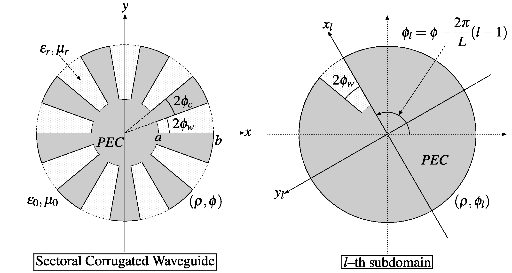
The geometry of the sectoral corrugated waveguide is shown in Figure 1. The waveguide is equally divided into L identical sectors, each consisting of a perfect electric conductor (PEC) region and a dielectric region characterized by ${\epsilon }_1={\epsilon }_r{\epsilon }_0$ and ${\mu }_1={\mu }_r{\mu }_0$. The inner and outer radii of the waveguide are a and b, and the central angles of PEC and dielectric sectors are $2{\varphi }_c$ and $2{\varphi }_w$, respectively. The waveguide is surrounded by free space.

The subdomain method decomposes the waveguide into L subdomains, one of which is illustrated in Figure 1. In the l-th subdomain ($l=1,2,\dots ,L$), all dielectric regions except for the l-th dielectric sector are replaced by PEC regions. The PEC replacement in each subdomain is not a physical approximation of the original structure; it is an auxiliary domain-decomposition device used to construct a coupled formulation. Because the governing equations and boundary conditions are linear in the phasor domain, the total fields of the original L-sector waveguide can be represented as a superposition of (i) the fields solved in each subdomain and (ii) coupling (auxiliary) fields introduced to enforce the original inter-sector boundary conditions. This assembly is explicitly enforced through the coupled boundary condition in (13).

The electromagnetic fields in each subdomain are represented in terms of the local coordinates $(\rho ,{\varphi }_l$), which are rotated by $2\pi (l-1)/L$ with respect to the global coordinates ($\rho ,\varphi$).

2.1. Field Representation

In the u-th subdomain ($u=1,2,\dots ,L$), the dielectric sector is defined over $a\le \rho \le b$ and $0\le {\varphi }_u\le 2{\varphi }_w$ where ${\varphi }_u$ denotes the local coordinates of the u-th subdomain. The longitudinal electromagnetic fields in the dielectric region are expressed as follows:

$$\begin{array}{cc}\hfill E_z^{I_u}& =\sum _{m=1}^{\infty }{A}_{m,u}^{TM}{R}_{{\nu }_m}^{TM}\left({\kappa }_1\rho \right)\sin {\nu }_m{\varphi }_u\hfill \end{array}$$

(1)

$$\begin{array}{cc}\hfill H_z^{I_u}& =\sum _{m=0}^{\infty }{A}_{m,u}^{TE}{R}_{{\nu }_m}^{TE}\left({\kappa }_1\rho \right)\cos {\nu }_m{\varphi }_u\hfill \end{array}$$

(2)

where ${\kappa }_1=\sqrt{k_1^2-{\beta }^2}$, $k_1=\omega \sqrt{{\mu }_1{\epsilon }_1}$ is the wavenumber in the dielectric region; $\beta$ is the phase constant, and

$${\nu }_m={\displaystyle \frac{m\pi }{2{\varphi }_w}}$$

(3)

$$\begin{array}{cc}\hfill R_{{\nu }_m}^{TM}\left({\kappa }_1\rho \right)& =J_{{\nu }_m}\left({\kappa }_1\rho \right)-{\displaystyle \frac{J_{{\nu }_m}\left({\kappa }_{1}a\right)}{N_{{\nu }_m}\left({\kappa }_{1}a\right)}}{N}_{{\nu }_m}\left({\kappa }_1\rho \right)\hfill \end{array}$$

(4)

$$\begin{array}{cc}\hfill R_{{\nu }_m}^{TE}\left({\kappa }_1\rho \right)& =J_{{\nu }_m}\left({\kappa }_1\rho \right)-{\displaystyle \frac{J_{{\nu }_m}^{\prime }\left({\kappa }_{1}a\right)}{N_{{\nu }_m}^{\prime }\left({\kappa }_{1}a\right)}}{N}_{{\nu }_m}\left({\kappa }_1\rho \right)\hfill \end{array}$$

(5)

Here, $J_{\nu }(·)$ and $N_{\nu }(·)$ are the Bessel functions of the first and second kinds, respectively. A prime (′) indicates the differentiation with respect to the argument (i.e., $J_{\nu }^{\prime }\left(x\right)=d{J}_{\nu }\left(x\right)/dx$).

$R_{{\nu }_m}^{TM/TE}\left({\kappa }_1\rho \right)$ are chosen to satisfy the Dirichlet and Neumann boundary conditions on $\rho =a$. When $a=0$, $R_{{\nu }_m}^{TM/TE}\left({\kappa }_1\rho \right)$ reduces to $J_{{\nu }_m}\left({\kappa }_1\rho \right)$.

The exterior fields consist of two parts. The first part is defined over $0\le {\varphi }_u\le 2{\varphi }_w$ and $\rho \ge b$, which is written as

$$\begin{array}{cc}\hfill E_z^{W_u}& =\sum _{m=1}^{\infty }{B}_{m,u}^{TM}{H}_{{\nu }_m}^{\left(2\right)}\left({\kappa }_0\rho \right)\sin {\nu }_m{\varphi }_u\hfill \end{array}$$

(6)

$$\begin{array}{cc}\hfill H_z^{W_u}& =\sum _{m=0}^{\infty }{B}_{m,u}^{TE}{H}_{{\nu }_m}^{\left(2\right)}\left({\kappa }_0\rho \right)\cos {\nu }_m{\varphi }_u,\hfill \end{array}$$

(7)

where $H_{\nu }^{\left(2\right)}(·)$ is the Hankel function of the second kind, ${\kappa }_0=\sqrt{k_0^2-{\beta }^2}$, and $k_0=\omega \sqrt{{\mu }_0{\epsilon }_0}$ is the wavenumber in free space. With $e^{j\omega t}$ convention, we take ${\kappa }_0=-j\sqrt{{\beta }^2-k_0^2}$ for bound modes ($\beta >k_0$) to ensure radial decay.

The second part of the exterior fields is induced to compensate for discontinuities of the $\widehat{\rho }$ and $\widehat{z}$ components of the magnetic field for $\rho >b$ and ${\varphi }_u=0$, $2{\varphi }_w$, in which the discontinuities are due to (6) and (7) [9,10]:

$$\begin{array}{cc}\hfill E_z^{C_u}={\displaystyle \frac{1}{j4}}\sum _{m=1}^{\infty }{B}_{m,u}^{TM}{\nu }_m& \sum _{n=0}^{\infty }(2-{\delta }_{n0})\left[J_n\left({\kappa }_0\rho \right)+C_n^{TM}{H}_n^{\left(2\right)}\left({\kappa }_0\rho \right)\right]I_{{\nu }_m,n}\hfill \\ & \times \left[\cos n{\varphi }_u-{(-1)}^m\cos n({\varphi }_u-2{\varphi }_w)\right]\hfill \end{array}$$

(8)

$$\begin{array}{cc}\hfill H_z^{C_u}=-{\displaystyle \frac{1}{j2}}\sum _{m=0}^{\infty }{B}_{m,u}^{TE}& \sum _{n=1}^{\infty }n\left[J_n\left({\kappa }_0\rho \right)+C_n^{TE}{H}_n^{\left(2\right)}\left({\kappa }_0\rho \right)\right]I_{{\nu }_m,n}\hfill \\ & \times \left[\sin n{\varphi }_u-{(-1)}^m\sin n({\varphi }_u-2{\varphi }_w)\right]\hfill \end{array}$$

(9)

where ${\delta }_{n0}$ is the Kronecker delta function, and

$$I_{{\nu }_m,n}={\int }_{{\rho }^{\prime }=b}^{\infty }{\displaystyle \frac{1}{{\rho }^{\prime }}}{H}_{{\nu }_m}^{\left(2\right)}\left({\kappa }_0{\rho }^{\prime }\right)H_n^{\left(2\right)}\left({\kappa }_0{\rho }^{\prime }\right)d{\rho }^{\prime }$$

(10)

$$\begin{array}{cc}\hfill C_n^{TM}& =-{\displaystyle \frac{J_n\left({\kappa }_{0}b\right)}{H_n^{\left(2\right)}\left({\kappa }_{0}b\right)}}\hfill \end{array}$$

(11)

$$\begin{array}{cc}\hfill C_n^{TE}& =-{\displaystyle \frac{J_n^{\prime }\left({\kappa }_{0}b\right)}{{H_n^{\left(2\right)}}^{\prime }\left({\kappa }_{0}b\right)}}\hfill \end{array}$$

(12)

The integral in (10) is evaluated in closed form, and the L’Hôpital’s rule is applied when ${\nu }_m\to n$. The explicit expression can be found in [9,10].

The transverse electric fields can be obtained using the transverse field relations in [12].

2.2. Boundary Conditions

The boundary condition of $E_z$ for $\rho =b$ and $0\le \varphi \le 2\pi$ can be divided into L independent conditions in the local coordinates as follows:

$$E_z^{I_u}=E_z^{W_u}+\sum _{l=1}^L{E}_z^{C_l},0\le {\varphi }_u\le 2{\varphi }_w$$

(13)

Since $E_z^{C_l}=0$ on $\rho =b$, the boundary condition in (13) reduces to $E_z^{I_u}=E_z^{W_u}$. Applying the orthogonality of $\sin {\nu }_p{\varphi }_u$ ($p>0$) gives the following:

$$A_{p,u}^{TM}={\displaystyle \frac{H_{{\nu }_p}^{\left(2\right)}\left({\kappa }_{0}b\right)}{R_{{\nu }_p}^{TM}\left({\kappa }_{1}b\right)}}{B}_{p,u}^{TM}$$

(14)

The boundary condition of $H_z$ for $\rho =b$ and $0\le {\varphi }_u\le 2{\varphi }_w$ is $H_z^{I_u}=H_z^{W_u}+{\sum }_{l=1}^L{H}_z^{C_l}$. The Wronskian of the Bessel functions and the orthogonality of $\cos {\nu }_p{\varphi }_u$ ($p\ge 0$) result in the following:

$$\begin{array}{cc}\hfill A_{p,u}^{TE}& ={\displaystyle \frac{H_{{\nu }_p}^{\left(2\right)}\left({\kappa }_{0}b\right)}{R_{{\nu }_p}^{TE}\left({\kappa }_{1}b\right)}}{B}_{p,u}^{TE}+{\displaystyle \frac{(2-{\delta }_{p0})}{\pi {\kappa }_{0}b{\varphi }_w}}{\displaystyle \frac{1}{R_{{\nu }_p}^{TE}\left({\kappa }_{1}b\right)}}\sum _{l=1}^L\sum _{m=0}^{\infty }{B}_{m,u}^{TE}\sum _{n=1}^{\infty }{\displaystyle \frac{n{I}_{{\nu }_m,n}{\Delta }_{{\nu }_p,n}^{u,l,m}}{{H_n^{\left(2\right)}}^{\prime }\left({\kappa }_{0}b\right)}},\hfill \end{array}$$

(15)

where

$$\begin{array}{cc}\hfill {\Delta }_{{\nu }_p,n}^{u,l,m}& ={\int }_{{\varphi }_u=0}^{2{\varphi }_w}\sin n{\varphi }_l\cos {\nu }_p{\varphi }_{u}d{\varphi }_u-{(-1)}^m{\int }_{{\varphi }_u=0}^{2{\varphi }_w}\sin n({\varphi }_l-2{\varphi }_w)\cos {\nu }_p{\varphi }_{u}d{\varphi }_u.\hfill \end{array}$$

(16)

Note that two different local coordinates exist in (16), and the integral is carried out with respect to ${\varphi }_u$. Hence, ${\varphi }_l$ must be transformed into ${\varphi }_u$ to obtain the closed form in (16). We define ${\varphi }_l={\varphi }_u-2{\varphi }_{\alpha }^{u,l}$, where

$${\varphi }_{\alpha }^{u,l}={\displaystyle \frac{\pi }{L}}(l-u)=({\varphi }_c+{\varphi }_w)(l-u).$$

(17)

This coordinate transformation allows integration in a common angular domain.

Similar to the boundary condition of $E_z$, that of $E_{\varphi }$ is given by $E_{\varphi }^{I_u}=E_{\varphi }^{W_u}$. The orthogonality of $\cos {\nu }_p{\varphi }_u$ ($p\ge 0$) and the substitution (15) into the boundary condition produce the following:

$$\begin{array}{cc}\hfill & \left[{\displaystyle \frac{{\mu }_1}{{\kappa }_1}}{\displaystyle \frac{{R_{{\nu }_p}^{TE}}^{\prime }\left({\kappa }_{1}b\right)}{R_{{\nu }_p}^{TE}\left({\kappa }_{1}b\right)}}{H}_{{\nu }_p}^{\left(2\right)}\left({\kappa }_{0}b\right)-{\displaystyle \frac{{\mu }_0}{{\kappa }_0}}{H_{{\nu }_p}^{\left(2\right)}}^{\prime }\left({\kappa }_{0}b\right)\right]B_{p,u}^{TE}\hfill \\ \hfill & +{\displaystyle \frac{(2-{\delta }_{p0})}{\pi {\kappa }_{0}b{\varphi }_w}}{\displaystyle \frac{{\mu }_1}{{\kappa }_1}}{\displaystyle \frac{{R_{{\nu }_p}^{TE}}^{\prime }\left({\kappa }_{1}b\right)}{R_{{\nu }_p}^{TE}\left({\kappa }_{1}b\right)}}\sum _{l=1}^L\sum _{m=0}^{\infty }{B}_{m,u}^{TE}\sum _{n=1}^{\infty }{\displaystyle \frac{n{I}_{{\nu }_m,n}{\Delta }_{{\nu }_p,n}^{u,l,m}}{{H_n^{\left(2\right)}}^{\prime }\left({\kappa }_{0}b\right)}}\hfill \\ \hfill & +(1-{\delta }_{p0}){\displaystyle \frac{\beta {\nu }_p}{\omega b}}\left[{\displaystyle \frac{1}{{\kappa }_1^2}}-{\displaystyle \frac{1}{{\kappa }_0^2}}\right]H_{{\nu }_p}^{\left(2\right)}\left({\kappa }_{0}b\right)B_{p,u}^{TM}=0\hfill \end{array}$$

(18)

Finally, the boundary condition of $H_{\varphi }$ with the Wronskian of the Bessel functions, the orthogonality of $\sin {\nu }_p{\varphi }_u$ ($p>0$), and the substitution of (14) and (15) yields the following:

$$\begin{array}{cc}\hfill & {\displaystyle \frac{\beta {\nu }_p}{\omega b}}\left[{\displaystyle \frac{1}{{\kappa }_1^2}}-{\displaystyle \frac{1}{{\kappa }_0^2}}\right]H_{{\nu }_p}^{\left(2\right)}\left({\kappa }_{0}b\right)B_{p,u}^{TE}\hfill \\ \hfill & +{\displaystyle \frac{\beta }{\pi \omega {\kappa }_0{b}^2}}\sum _{l=1}^L\sum _{m=0}^{\infty }{B}_{m,u}^{TE}\sum _{n=1}^{\infty }{\displaystyle \frac{I_{{\nu }_m,n}}{{H_n^{\left(2\right)}}^{\prime }\left({\kappa }_{0}b\right)}}\left[{\displaystyle \frac{2n{\nu }_p{\Delta }_{{\nu }_p,n}^{u,l,m}}{{\kappa }_1^2{\varphi }_w}}+{\displaystyle \frac{n^2{\Omega }_{{\nu }_p,n}^{u,l,m}}{{\kappa }_0^2}}\right]\hfill \\ \hfill & +\left[{\displaystyle \frac{{\epsilon }_1}{{\kappa }_1}}{\displaystyle \frac{{R_{{\nu }_p}^{TM}}^{\prime }\left({\kappa }_{1}b\right)}{R_{{\nu }_p}^{TM}\left({\kappa }_{1}b\right)}}{H}_{{\nu }_p}^{\left(2\right)}\left({\kappa }_{0}b\right)-{\displaystyle \frac{{\epsilon }_0}{{\kappa }_0}}{H_{{\nu }_p}^{\left(2\right)}}^{\prime }\left({\kappa }_{0}b\right)\right]B_{p,u}^{TM}\hfill \\ \hfill & -{\displaystyle \frac{{\epsilon }_0}{2\pi {\kappa }_0^{2}b}}\sum _{l=1}^L\sum _{m=1}^{\infty }{B}_{m,u}^{TM}{\nu }_m\sum _{n=0}^{\infty }{\displaystyle \frac{(2-{\delta }_{n0})I_{{\nu }_m,n}{\Omega }_{{\nu }_p,n}^{u,l,m}}{H_n^{\left(2\right)}\left({\kappa }_{0}b\right)}}\hfill \\ \hfill & =0,\hfill \end{array}$$

(19)

where

$$\begin{array}{cc}\hfill {\Omega }_{{\nu }_p,n}^{u,l,m}& ={\int }_{{\varphi }_u=0}^{2{\varphi }_w}\cos n{\varphi }_l\sin {\nu }_p{\varphi }_{u}d{\varphi }_u\hfill \\ \hfill & -{(-1)}^m{\int }_{{\varphi }_u=0}^{2{\varphi }_w}\cos n({\varphi }_l-2{\varphi }_w)\sin {\nu }_p{\varphi }_{u}d{\varphi }_u.\hfill \end{array}$$

(20)

The Equations (18) and (19) constitute the system equations of the sectoral corrugated waveguide. The determinant of this system defines the dispersion relation of the waveguide.

With the truncations ($m=0,\dots ,M$ for TE, and $m=1,\dots ,M$ for TM), each sector has $2M-1$ unknowns. Hence, the full system has size $L(2M-1)$. However, assembling (18) and (19) for all L sectors can yield a BCM system diagonalizable by the DFT; the problem decouples into L subproblems of size $2M-1$.

3. Numerical Results

The proposed method was evaluated for accuracy and efficiency. Due to azimuthal periodicity, the computed phase constants concentrate densely around specific values, thereby forming clusters. Hence, we validated accuracy using the median value of the phase constant (${\beta }_M$) of each cluster and compared it with COMSOL Multiphysics 6.2 [13] (hereafter, “COMSOL” refers to COMSOL Multiphysics 6.2). Efficiency was evaluated by comparing the elapsed time required by the BCM formulation, full matrix formulation, and COMSOL. Note that only guided modes of ${\beta }_M$ were considered in this study (i.e., $k_0<\beta <k_1$).

The dispersion relation was obtained by applying singular-value decomposition (SVD) to the system matrix formed by (18) and (19) and finding the smallest singular value ${\sigma }_{min}$. The phase constant, $\beta$, was then identified where ${\sigma }_{min}\approx 0$.

We sampled $\beta$ from $k_0$ to $k_1$ with a step of ${10}^{-3}$ to search for the points where ${\sigma }_{min}$ becomes small. Since Equations (18) and (19) contain infinite series for m and n, they must be truncated properly. Based on a convergence study, the computed ${\beta }_M$ was found to vary by less than $0.2\%$ when M was increased from 1 to 3 and N from 120 to 150 over the considered parameter range. Accordingly, $M=1$ ($m=0,1$ for TE and $m=1$ for TM) and $N=120$ were adopted to balance accuracy and computational efficiency.

The parameters of the basic test case were $a=0.15$, $b=1.0$, $2{\varphi }_w=6^{°}$, $L=24$, ${\epsilon }_r=4$, and ${\mu }_r=1$. In addition, we defined the filling fraction, $\xi$, as the ratio of the dielectric region to the single sector, which is given by the following:

$$\xi ={\displaystyle \frac{{\varphi }_w}{{\varphi }_w+{\varphi }_c}}$$

(21)

Based on the definition, the basic test case had a filling fraction of 0.4.

Finally, all experiments were performed on a MacBook Air (Apple M2, 8-core CPU, 24 GB unified memory).

3.1. Accuracy

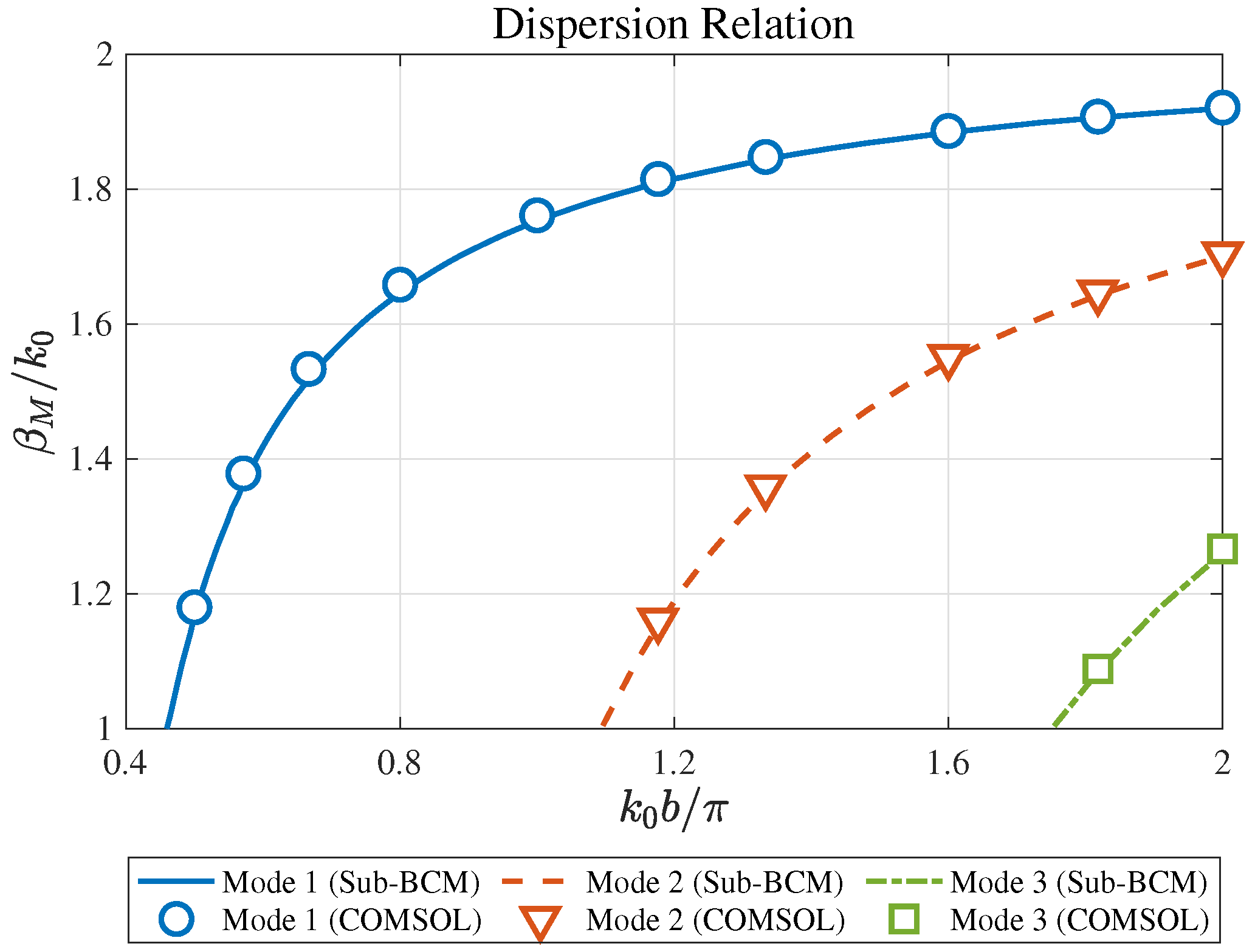
To verify the accuracy of the proposed method, we estimated ${\beta }_M$ of the clusters for a given geometry and constructed the dispersion relation of the sectoral corrugated waveguide. The median values of $\beta$ evaluated by the subdomain method using the BCM formulation were compared with those obtained by COMSOL, as shown in Figure 2. COMSOL results were evaluated at representative frequency points, which are indicated by markers in Figure 2, while the solid lines represent ${\beta }_M$ obtained by the proposed method. For all the sampled comparison points, the median values of the phase constants from the proposed method agree with COMSOL within 1.2%.

3.2. Efficiency

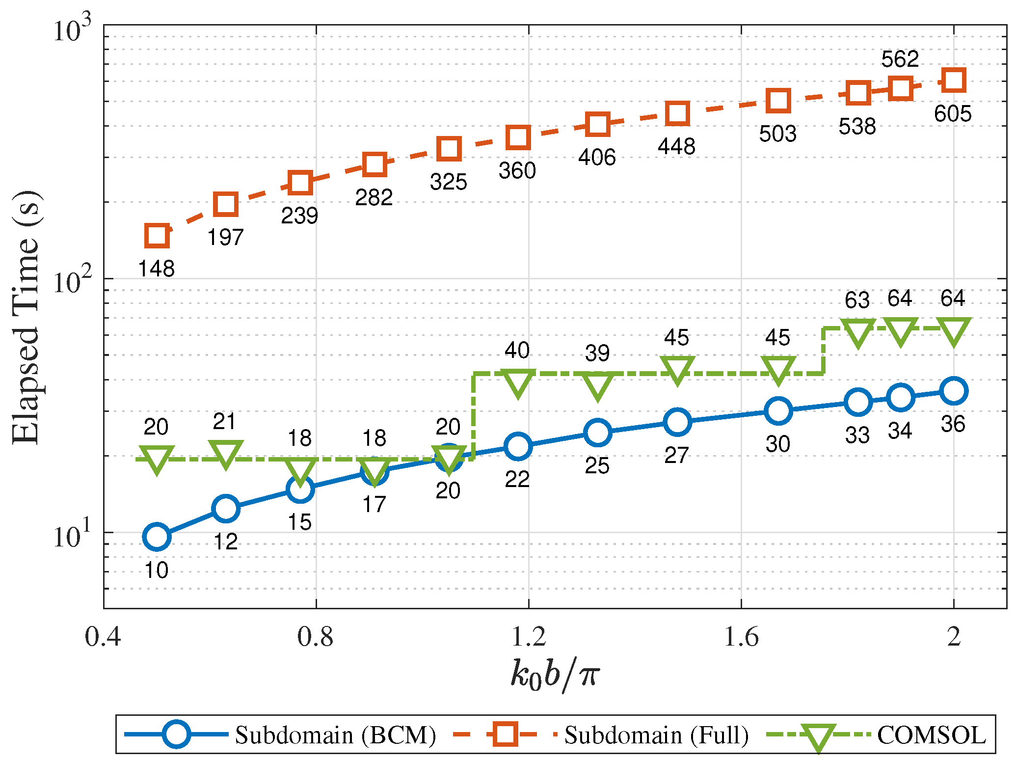
We measured the computation time of the BCM formulation, the full matrix formulation, and COMSOL to evaluate efficiency. Figure 3 compares the elapsed time as the number of propagating mode clusters increases. As shown in Figure 3, the BCM formulation is more efficient than both the full matrix formulation and COMSOL. The BCM formulation requires 6.0–6.5% of the computation time of the full matrix formulation. When comparing with COMSOL, the BCM formulation becomes more efficient as the number of propagating mode clusters increases. For the single cluster, the BCM formulation requires 47.9–98.7% of the computation time of COMSOL, while it reduces to 54.4–67.0% for two clusters, and 51.8–56.3% for three clusters.

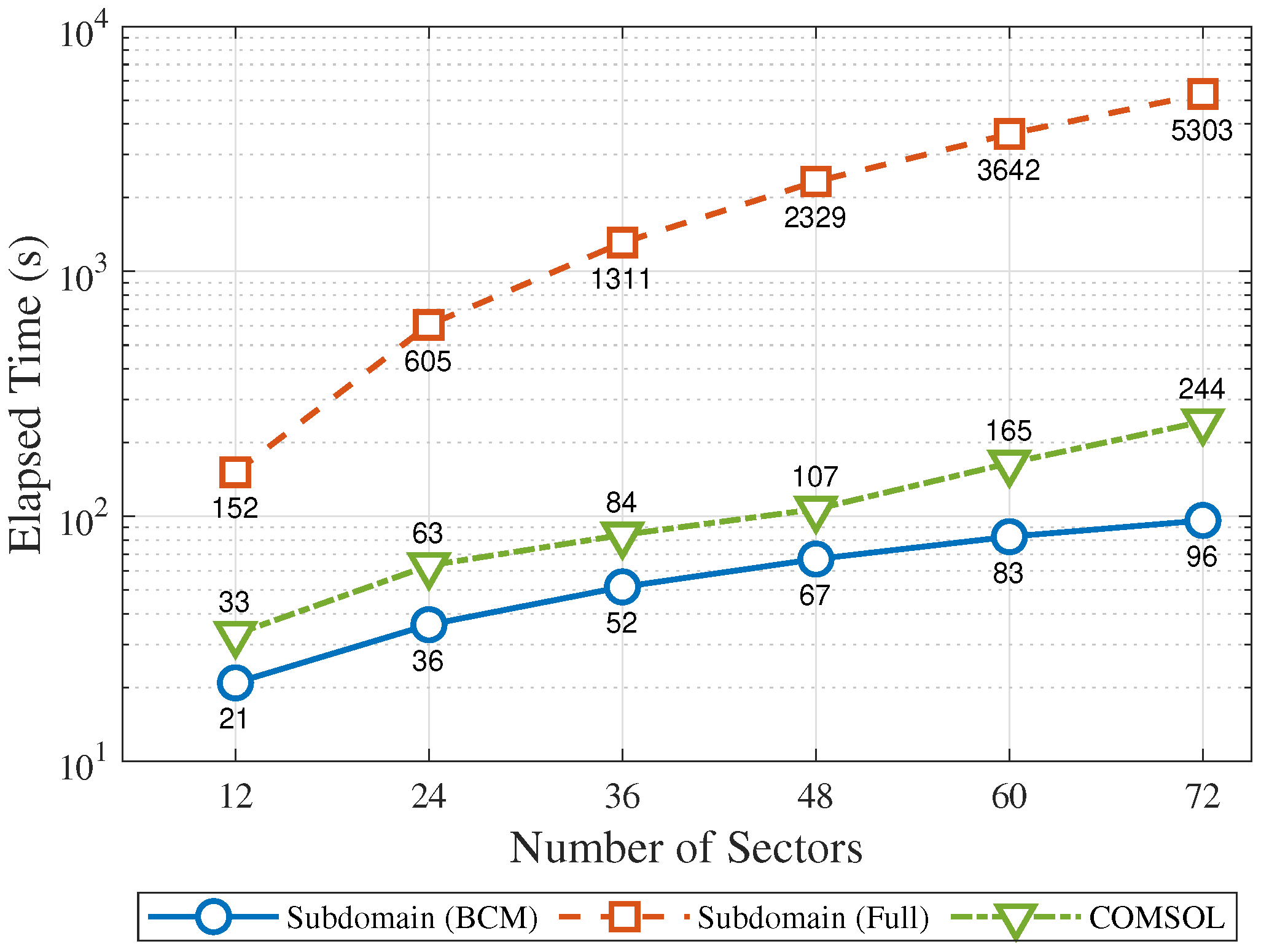
Figure 4 compares the elapsed time as the number of sectors L increases ($L=12,24,36,48,60,72$) while maintaining the filling fraction. The BCM formulation requires the least computation time among the three methods. The elapsed times of the BCM formulation and COMSOL increase approximately linearly with L, whereas that of the full matrix formulation increases quadratically. Overall, the BCM formulation requires 39.4–63.2% of the computation time of COMSOL and 1.8–13.8% of that of the full matrix formulation. These results indicate that the BCM formulation is advantageous for structures with a large number of sectors, where the full matrix formulation becomes prohibitive, and commercial solvers require increased computational cost.

4. Discussion

This study presented an efficient semi-analytical formulation for the dispersion analysis of sectoral corrugated waveguides by combining a subdomain representation in local coordinates with mode-matching at the sector interfaces. Compared with asymptotic boundary-condition or reduced-order treatments, the present approach preserves a full-wave mode-matching formulation while reducing the computational cost for azimuthally periodic structures. The key computational advantage originates from the block-circulant structure of the assembled system matrix, which naturally arises from the rotational periodicity of identical sectors. By exploiting this structure, the global problem of size $L(2M-1)$ can be decoupled into L independent subproblems of size $(2M-1)$ through the discrete Fourier transform (DFT), substantially reducing both computational time and memory requirements.

The numerical results indicate that the proposed formulation produces dispersion curves that agree well with those from a commercial full-wave solver, with a small relative error over the tested parameter ranges. In addition, the efficiency study shows that the block-circulant formulation becomes increasingly advantageous as the number of sectors increases, where a direct full-matrix approach exhibits quadratic growth in computational cost. These trends suggest that the proposed approach is particularly suitable for practical sectoral geometries with moderate-to-large L, where repeated dispersion evaluations are required, for example, during parametric sweeps or geometry optimization.

Several limitations should be noted. First, the current implementation assumes identical sectors and perfect rotational periodicity; deviations from periodicity (e.g., manufacturing tolerances or intentional sector-to-sector variations) would generally break the block-circulant symmetry and reduce the benefit of DFT-based decoupling. Second, accuracy and efficiency depend on appropriate truncation of the modal expansions and auxiliary series, and the required truncation levels may increase for higher frequencies or for geometries with sharper features. Third, the present study focused on guided modes in the range $k_0<\beta <k_1$; extending the framework to treat leaky or radiating modes may require solving for complex roots $\beta$ (and complex radial wavenumbers) in the complex plane, which is numerically more delicate than a real-valued root search.

Future work may consider extensions to include material losses, finite conductivity, or anisotropic/inhomogeneous sector fillings, as well as robust treatments for imperfect periodicity. Another practical direction is to couple the present formulation with automated parameter search and optimization, leveraging the reduced computational cost to enable rapid exploration of design spaces for sectoral corrugated waveguide components.