Article

Adaptive Edge-Aware Detection with Lightweight Multi-Scale Fusion

1
School of Electronic Information and Physics, Central South University of Forestry and Technology, Changsha 410004, China
2
School of Computer Science and Mathematics, Central South University of Forestry and Technology, Changsha 410004, China
*
Author to whom correspondence should be addressed.
Electronics 2026, 15(2), 449; https://doi.org/10.3390/electronics15020449
Submission received: 27 December 2025 / Revised: 18 January 2026 / Accepted: 19 January 2026 / Published: 20 January 2026
(This article belongs to the Topic Intelligent Image Processing Technology)

Abstract

In object detection, boundary blurring caused by occlusion and background interference often hinders effective feature extraction. To address this challenge, we propose Edge Aware-YOLO, a novel framework designed to enhance edge awareness and efficient feature fusion. Our method integrates three key contributions. First, the Variable Sobel Compact Inverted Block (VSCIB) employs convolution kernels with adjustable orientation and size, enabling robust multi-scale edge adaptation. Second, the Spatial Pyramid Shared Convolution (SPSC) replaces standard pooling with shared dilated convolutions, minimizing detail loss during feature reconstruction. Finally, the Efficient Downsampling Convolution (EDC) utilizes a dual-branch architecture to balance channel compression with semantic preservation. Extensive evaluations on public datasets demonstrate that Edge Aware-YOLO significantly outperforms state-of-the-art models. On MS COCO, it achieves 56.3% mAP50 and 40.5% mAP50–95 (gains of 1.5% and 1.0%) with only 2.4M parameters and 5.8 GFLOPs, surpassing advanced models like YOLOv11.

1. Introduction

Real-time object detection, as a significant research direction in the field of computer vision, has always garnered considerable attention. Its core objective is to rapidly and accurately predict the categories and locations of objects in images with low latency. This technology has demonstrated immense application potential in various real-world scenarios, such as the precise identification of vehicles and pedestrians in autonomous driving [1], environmental perception and obstacle avoidance in robot navigation [2], and dynamic object recognition and localization in target tracking [3], among others. The efficiency and reliability of real-time object detection directly determine the performance and safety of these applications.
In recent years, researchers have widely adopted convolutional neural network (CNN)-based object detection methods [4,5,6] to balance the trade-off between detection accuracy and speed, driving the advancement of real-time object detection. Among these, the YOLO (You Only Look Once) series of models has rapidly become a research hotspot in this field due to its unique single-stage detection architecture, achieving an ideal balance between performance and efficiency [7,8]. By employing an end-to-end detection pipeline, the YOLO series significantly reduces computational overhead. Its excellent performance in both speed and accuracy has led to its widespread adoption in applications such as autonomous driving, intelligent surveillance, and drone-based object detection.
In complex detection environments, edge information plays a pivotal role in ensuring system robustness and generalization. From the perspective of visual cognition, edges represent high-frequency structural components that possess geometric invariance, unlike texture or color features that are highly susceptible to illumination changes and environmental noise. Explicitly modeling edge orientation allows the network to decouple structural boundaries from background clutter, thereby enhancing (1) robustness, by maintaining stable feature responses even when texture information is degraded by blur or low light, and (2) generalization, as geometric contours are often domain-independent features that transfer better across different scenarios (e.g., from clear water to turbid water) than domain-specific textures. Despite this, most current real-time detectors rely on implicit feature learning, neglecting the explicit utilization of this critical geometric prior.
However, object detection models face multiple challenges in feature extraction and multi-scale processing. Conventional models [9,10] rely on fixed-parameter convolution kernels for feature extraction. Although computationally efficient, this design severely limits geometric adaptability, resulting in inefficient capture of blurred boundaries and multi-directional edge features in complex scenes. While improvements like deformable convolution [11] and large kernel attention [12] attempt to enhance spatial adaptability by learning sampling offsets or expanding receptive fields, they rely on implicit feature matching to predict these offsets. In scenarios with motion blur or low contrast (e.g., underwater environments), the gradient information is often too diffuse for the network to learn precise offsets, causing sampling points to drift towards noise or dominant background textures. Furthermore, these methods lack explicit modeling of edge orientation information, fundamentally limiting edge localization accuracy under background clutter interference where a strong geometric prior is essential.
Addressing multi-scale processing challenges, multi-scale feature fusion techniques have undergone continuous evolution yet still face performance trade-offs. Modules like Spatial Pyramid Pooling (SPP) [9] in YOLOv4, Atrous Spatial Pyramid Pooling (ASPP) [13] in DeepLab, and Spatial Pyramid Pooling Fast (SPPF) in YOLOv5 enhance multi-scale representation by aggregating features with different receptive fields. However, these modules face inherent trade-offs: SPP employs multi-scale pooling to capture context, but max-pooling inevitably neglects details in non-maximum regions. ASPP leverages parallel dilated convolutions with varying dilation rates to expand receptive fields, but its independent branch operations introduce excessive computational costs compared to single dilated convolution. SPPF optimizes SPP through cascaded pooling layers with identical kernel sizes followed by unified convolution, yet repeated pooling operations may amplify low-frequency noise in blurred object boundaries.
In object detection, feature map downsampling serves as a critical stage for balancing computational efficiency and feature representation capability. Existing convolution methods struggle to simultaneously achieve lightweight design, receptive field coverage, and feature integrity during development. Standard convolution [14] generates exponentially growing computational costs on deep high-dimensional feature maps, while irreversible information compression occurs during progressive downsampling. Depthwise separable convolution [15] significantly reduces computational costs, but its limited receptive fields and lack of global context awareness hinder effective balance between feature compression and information extraction. Dilated convolution [16] expands receptive fields through sparse sampling, yet its low computational efficiency makes it unsuitable for high-efficiency downsampling tasks. Traditional grouped convolution [17] reduces parameter count via channel grouping, but weak cross-group interaction and feature fusion capabilities often lead to inadequate feature representation.
To address the aforementioned challenges, this paper proposes Edge Aware-YOLO—a YOLOv11-based framework integrating adaptive edge awareness and efficient feature fusion, achieving optimal balance between high accuracy and lightweight design. The main contributions are summarized as follows:
1.
Addressing geometric constraints in edge extraction:To overcome the limitations of traditional Sobel operators, which are restricted to fixed scales and discrete orientations, we propose the Variable Sobel Compact Inverted Block (VSCIB). By dynamically adjusting kernel size and orientation, this module significantly enhances the model’s ability to capture multi-scale and multi-directional edge features.
2.
Optimizing feature fusion efficiency:Targeting the detail loss and redundancy caused by standard pooling operations, we introduce the Spatial Pyramid Shared Convolution (SPSC). This module replaces pooling with shared dilated convolutions, effectively preserving multi-scale information while avoiding unnecessary computational overhead.
3.
Reducing downsampling loss: To mitigate severe semantic information loss during feature map reduction, we design the Efficient Downsampling Convolution (EDC). Utilizing a dual-branch architecture to balance compression and preservation, it substantially reduces parameter count and GFLOPs without compromising detection performance.

2. Related Works

This section reviews the foundational technologies and recent advancements that underpin our proposed framework. We begin by examining the evolution of the YOLO series to establish the context of the baseline architecture used in this study. Subsequently, we delve into existing methodologies for edge feature extraction and spatial pyramid feature fusion. By analyzing the limitations of current approaches in terms of boundary perception and computational efficiency, we define the research gaps that motivate the design of our Edge Aware-YOLO and its constituent modules (VSCIB, SPSC, and EDC).

2.1. You Only Look Once (YOLO)-11

The YOLO series has consistently served as the cornerstone of real-time object detection, evolving from the single-stage YOLOv1 [18] to the optimized YOLOv11 [19]. Each iteration has introduced significant structural advancements. For instance, YOLOv4 focused on structural refinement, while YOLOv7 [20] achieved breakthroughs in speed and performance via the E-ELAN backbone. Subsequent models introduced diverse mechanisms: YOLOX [21] adopted an anchor-free approach to enhance flexibility, whereas Gold-YOLO improved feature fusion through its gather-and-distribute mechanism.
Despite competition from emerging detectors like RT-DETR [22], YOLO maintains widespread adoption due to its robust feature integration techniques, such as CSPNet, ELAN [23], and enhanced PANet [24] or FPN [25]. Additionally, detection accuracy has been boosted by complex prediction heads inspired by YOLOv3 [26] and FCOS. Recent iterations have further pushed the limits: YOLOv9 [27] minimized information loss using programmable gradient information, while YOLOv10 [28] set a new benchmark for efficiency by eliminating non-maximum suppression (NMS).
In this study, we select YOLOv11n as the baseline. It offers an optimal trade-off between high efficiency and competitive accuracy, making it ideal for resource-constrained scenarios with stringent speed requirements.

2.2. Edge Feature Extraction

With the advancement of deep learning, CNN-based edge feature extraction has become mainstream. While convolutional operations excel at general feature extraction, their fixed kernels lack orientation sensitivity, making it difficult to optimize specifically for edge features. To address this, methods such as dynamic convolution [29] and deformable convolution [30] were introduced. Although these approaches improve representation through dynamic weights or flexible sampling, they still struggle with precise edge perception. Specifically, dynamic convolution uses multi-kernel attention to adjust weights, yet it lacks explicit orientation modeling. This often results in discretized responses along slender, curved edges (e.g., vascular branches). Similarly, while deformable convolution adjusts sampling grids via offsets, its global computation strategy is inefficient for edges: uniformly distributed offsets dilute the focus on critical boundary regions and remain susceptible to noise in complex scenarios (e.g., airport pavement cracks).
Hybrid approaches combining classical edge detection with deep learning have also been explored, such as using Sobel or Laplacian operators for preprocessing. While these methods offer moderate improvements, the generated low-level edge features fail to integrate effectively with the high-level semantic features of deep networks. Furthermore, traditional operators tend to amplify noise (e.g., the Laplacian’s high-frequency sensitivity), forcing subsequent networks to perform additional denoising, which ultimately compromises the overall detection performance.

2.3. Spatial Pyramid Feature Fusion

Spatial Pyramid Feature Fusion is a widely used technique in object detection and semantic segmentation tasks, aiming to enhance the model’s receptive field and perception of objects at different scales through multi-scale feature fusion. Early modules such as Spatial Pyramid Pooling (SPP) and Atrous Spatial Pyramid Pooling (ASPP) extract features at multiple scales using pooling operations or dilated convolutions, then concatenate and fuse these features to improve the model’s ability to detect objects of varying sizes. However, these modules typically suffer from the following limitations: (1) high computational complexity and (2) parameter redundancy.
In recent years, some improvements have attempted to optimize spatial pyramid modules by reducing computational overhead. For example, the Receptive Field Block (RFB) [30] and SPPF modules accelerate inference by reducing the number of dilated convolutions or pooling operations. However, the feature fusion capabilities of these methods remain limited, making it difficult to fully capture multi-scale information in complex scenes while maintaining efficiency.

3. Proposed Approach

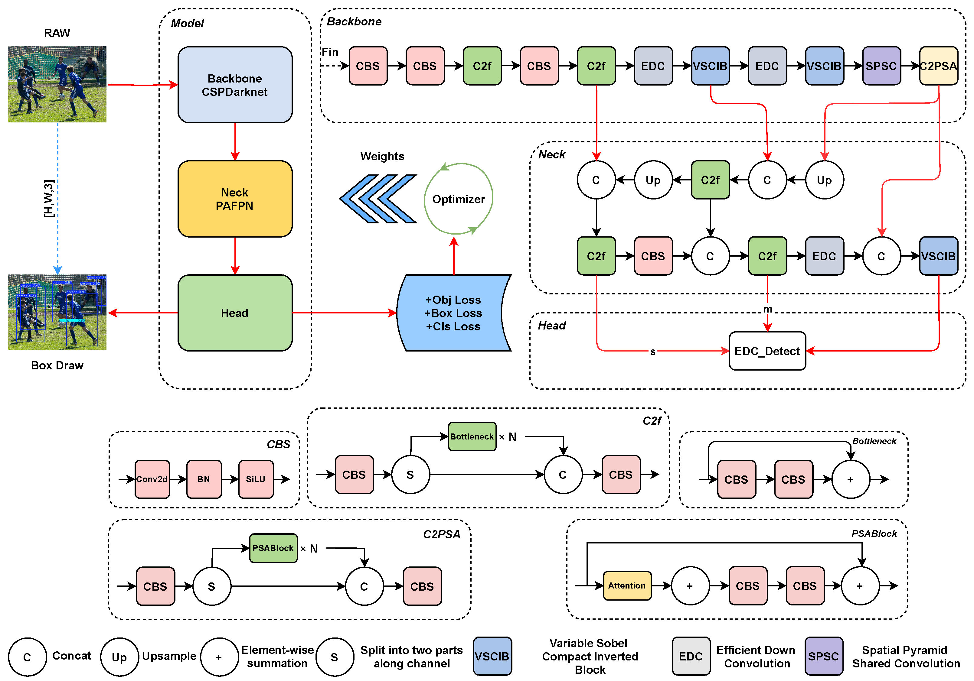
This section details the architectural innovations of the proposed Edge Aware-YOLO, which integrates three strategic components to balance detection accuracy and computational efficiency. First, the Variable Sobel Compact Inverted Block (VSCIB) is designed to enhance feature adaptability, specifically addressing boundary blurring in complex scenarios. Second, the Spatial Pyramid Shared Convolution (SPSC) is employed to capture rich multi-scale context while suppressing isolated noise. Finally, the Efficient Downsampling Convolution (EDC) replaces conventional heavy layers to minimize parameter redundancy without compromising performance. Adhering to a modular design philosophy, these components ensure flexibility and scalability. The overall network architecture is illustrated in Figure 1.

3.1. Baseline

The baseline utilizes the fundamental architecture of the YOLOv11 model, which primarily consists of four core components: Input, Backbone, Neck, and Head. First, the image is sent to the input layer, where it undergoes preprocessing such as data augmentation before being passed to the backbone network to extract features from the processed image. Then, the neck network uses feature fusion to create feature maps of large, medium, and small sizes from the retrieved data. Finally, the detection head receives the refined features and provides predictions for three different-sized anchor boxes after detection.

3.2. Variable Sobel Compact Inverted Block

Existing modules exhibit insufficient sensitivity to edge feature extraction. Therefore, we propose the Variable Sobel Compact Inverted Block (VSCIB) leveraging Sobel operators to enable superior edge information comprehension. The VSCIB module reconstructs feature extraction flow based on the C3k/C3k2 architecture, with its core comprising collaborative Variable Sobel Convolution (VSC) and Compact Inverted Block (CIB). As shown in Figure 2, the module first processes input feature maps through the VSC submodule, which performs edge detection using Sobel operators and generates multi-directional edge features via matrix rotation for multi-scale edge information capture. Simultaneously, the CIB submodule employs an optimized inverted residual structure to enable inter-channel interaction and feature fusion, conducting channel-wise fusion between processed features and original inputs. This is followed by cascaded operations of channel compression and restoration for feature dimensionality reduction/expansion, ultimately enhancing edge detail representation through residual connections while preserving original input information.
In our design, the VSC module generates oriented Sobel kernels through rotational transformations of a base kernel. For a kernel size L, we define the optimal smoothing operator coefficients S m = [ S 0 , S 1 , , S L 1 ] and differential operator coefficients D m = [ D 0 , D 1 , , D L 1 ] as:
S m = ( L 1 ) ! ( L 1 m ) ! m ! for m = 0 , 1 , , L 1
D m = P pascal ( m , L 2 ) P pascal ( m 1 , L 2 )
where the Pascal triangle function is defined as
P pascal ( k , r ) = r ! ( r k ) ! k ! 0 k r 0 otherwise
It is important to note that the Sobel kernel is constructed by the outer product of a smoothing vector S m and a difference vector D m . The inclusion of S m (Equation (1)) effectively acts as a low-pass filter, suppressing high-frequency texture noise before the gradient calculation. This ensures that VSCIB remains robust even in noisy environments, addressing the common concern that gradient-based features might amplify noise.
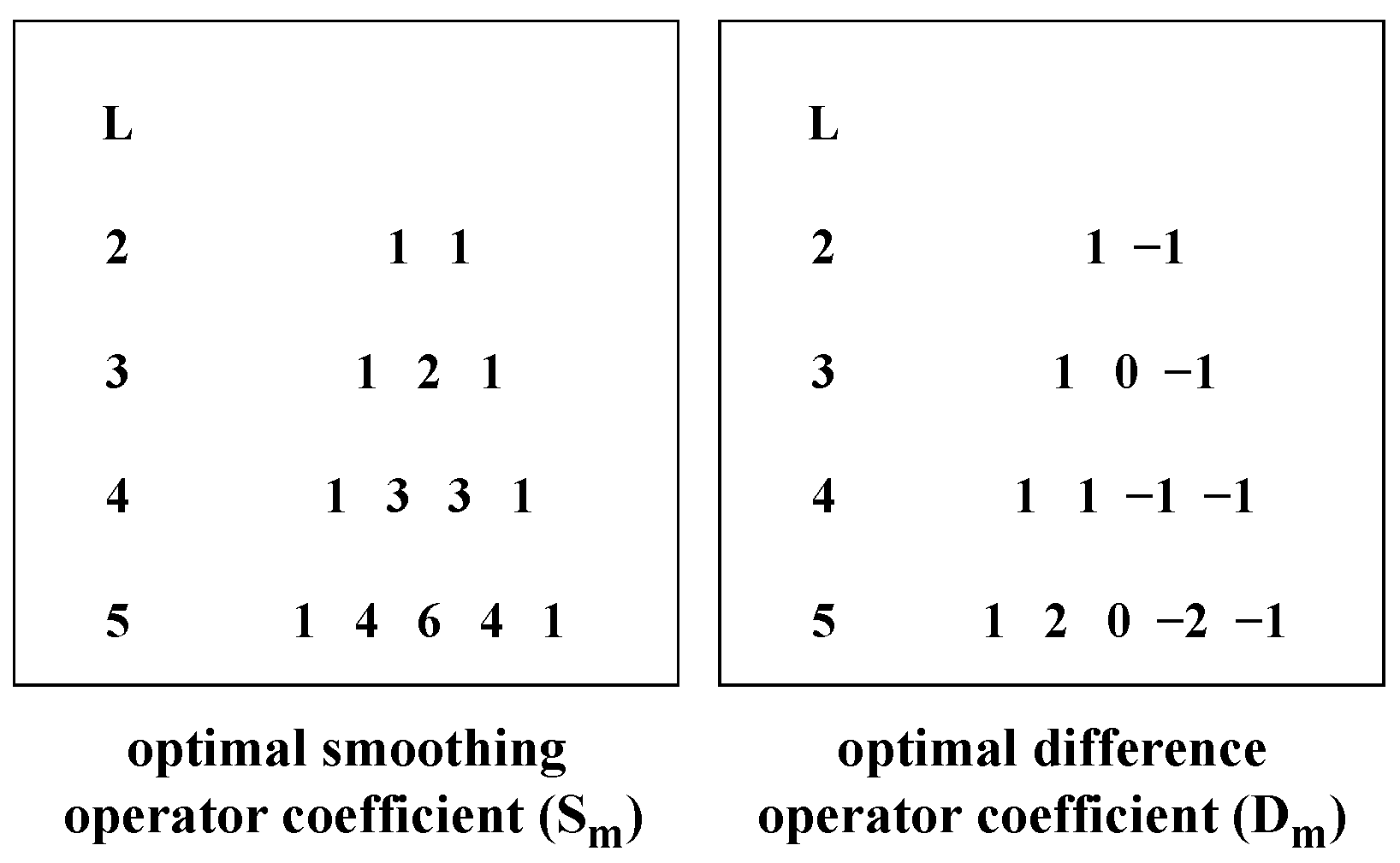
Figure 3 visually presents the two key matrices containing the optimal smoothing operator coefficient S m and the optimal difference operator coefficient D m , where L represents the window size. The figure clearly displays how these coefficients vary for different window sizes (L = 2, 3, 4, 5), with the smoothing coefficients shown on the left and difference coefficients on the right. For example, when L = 2, the smoothing coefficients are [1, 1] and the difference coefficients are [1, −1].
The base Sobel kernel for 0° orientation is obtained through the outer product:
Sobel M ( 0 ) = m = 0 L 1 n = 0 L 1 S m D n for m , n = 0 , 1 , , L 1
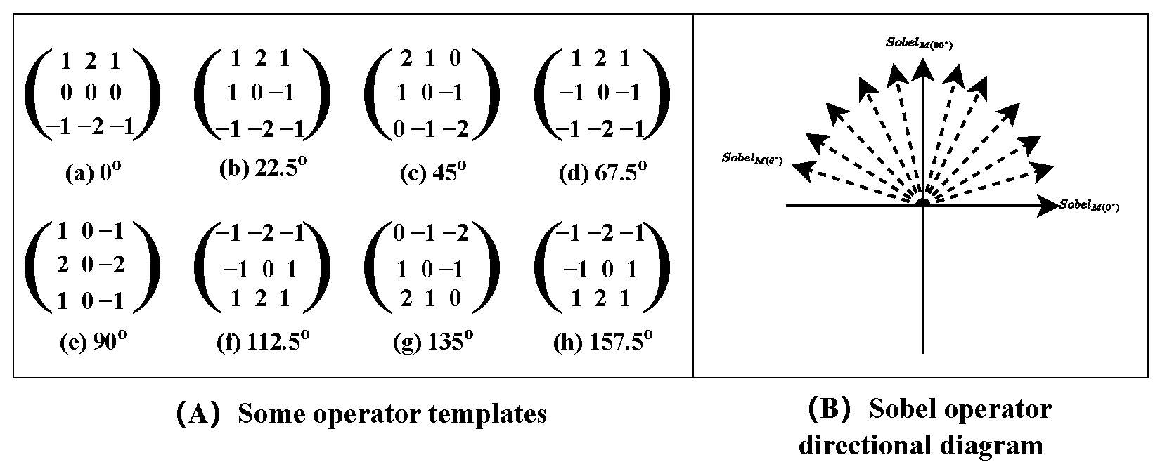
Figure 4 demonstrates the complete set of 3 × 3 Sobel operator templates for 8 different orientations, covering directions from 0° to 157.5° at 22.5° intervals. The left portion (A) of the figure displays the actual operator templates for each orientation, while the right portion (B) provides a directional diagram illustrating the application directions of these Sobel operators. These templates are generated by applying our rotation algorithm to the base kernel, enabling multi-directional edge detection capabilities that are essential for robust underwater image processing. The comprehensive orientation coverage ensures that our method can effectively capture edge features from various directions, which is particularly important for detecting underwater objects with complex shapes and orientations.
Comparison with Adaptive Convolutions. It is essential to distinguish the advantage of VSCIB over adaptive methods like deformable convolution networks (DCN). DCN enhances geometric adaptability by learning offsets for sampling points via an additional convolutional layer. However, this implicit learning process is highly sensitive to input quality. In scenarios with blurred edges or low contrast (typical in underwater or defect detection), the gradient information is often too diffuse for the network to learn precise offsets, causing sampling points to drift towards noise or dominant background textures.
In contrast, VSCIB incorporates a strong explicit geometric prior. By mathematically defining the smoothing operator S m (Equation (1)) and the differential operator D m (Equation (2)), VSCIB effectively functions as a “Smoothing + Differencing” mechanism. The smoothing term S m acts as a low-pass filter to suppress high-frequency noise, ensuring that the subsequent gradient calculation targets structural edges rather than textural noise. This makes VSCIB significantly more robust than learned offsets in degraded environments. Furthermore, since the kernel rotation is deterministic, VSCIB avoids the heavy computational overhead of predicting per-pixel offset fields required by DCN, maintaining higher inference efficiency.
Kernels for arbitrary orientations θ are generated using the optimized rotation logic described in Algorithm 1. To ensure precise alignment and avoid geometric distortion, we employ an inverse mapping strategy. For each coordinate in the target rotated kernel R , we calculate its corresponding position in the base kernel M using a rotation matrix centered at c = L / 2 . As shown in Step 4 of the algorithm, this coordinate transformation is mathematically rigorous. Subsequently, a nearest-neighbor interpolation (Steps 5–7) is applied to assign values, ensuring that the discrete integer properties of the Sobel operator are preserved while preventing coordinate shift accumulation.
Algorithm 1 Optimized Algorithm for Sobel Kernel Rotation
Input: Base Kernel M R L × L , Rotation Angle θ
Output: Rotated Kernel R R L × L
1:      c L / 2    // Kernel center
2:      R 0 L × L    // Initialize output
3:     foreach pixel ( i , j ) in R  do
4:        Compute source coordinates ( x , y ) relative to center:
            x y cos θ sin θ sin θ cos θ i c j c + c c
5:         x n n round ( x ) , y n n round ( y )    // Nearest neighbor
6:        if  0 x n n < L  and  0 y n n < L  then
7:            R [ i , j ] M [ x n n , y n n ]
8:        end if
9:     end for
10:   return R
The Compact Inverted Block (CIB) employs an inverted residual structure with an expansion ratio e (default e = 1 ) to facilitate efficient feature fusion. The CIB first expands the channel dimension, applies depthwise separable convolution for spatial feature extraction, and subsequently compresses channels back to the original dimensionality, followed by a residual connection with the input features. The output of VSCIB integrates multi-orientation edge features from VSC and contextual features from CIB through normalized fusion:
x 1 = x + DWConv ( CBS ( DWConv ( CBS ( DWConv ( x ) ) ) ) )
x 2 = x + CBS ( Concat ( x , ( 1 N θ = 0 N 1 Sobel M ( θ ) ( x ) , x 1 ) ) )
x out = x + CBS ( CBS ( x 2 ) )
where x denotes input features, CBS represents Conv-BN-SiLU operations, DWConv indicates depthwise separable convolution, and N is the number of orientations. This design enables complementary enhancement of edge details and semantic context through multi-path feature integration.
  • Synergistic Design Integration. The architectural logic of our framework relies on the complementary relationship between feature enhancement and structural efficiency. While the VSCIB module significantly improves the network’s sensitivity to high-frequency edge information and semantic context, this enriched representation risks degradation if subjected to standard, lossy downsampling operations (such as Max Pooling or strided convolutions). Furthermore, the computational investment made in the VSCIB for precise edge extraction necessitates a subsequent reduction in spatial redundancy to maintain overall model lightness. Consequently, the design transitions to the Efficient Downsampling Convolution (EDC). This module serves as the structural counterpart to VSCIB, ensuring that the integrity of the extracted edge features is preserved during dimensionality reduction while effectively offsetting computational costs through its streamlined dual-branch architecture.

3.3. Efficient Downsampling Convolution

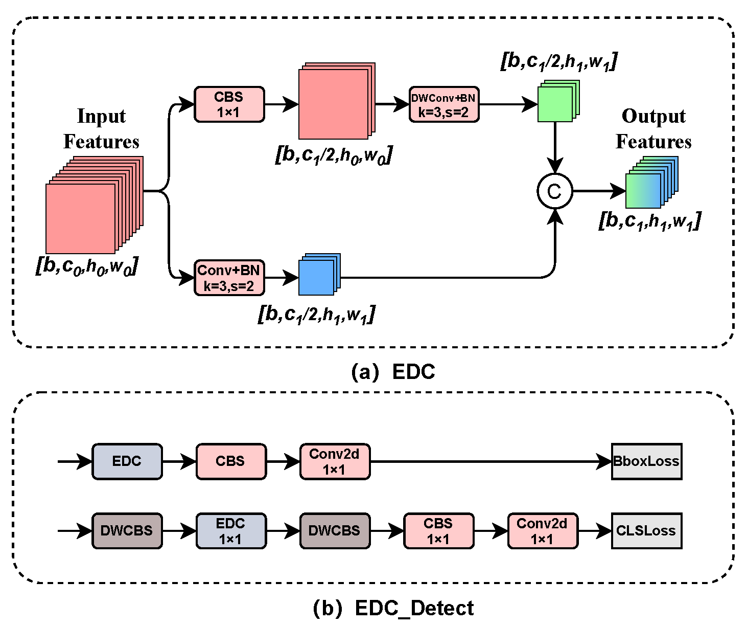
To address information loss and computational inefficiency in standard downsampling, we propose the Efficient Downsampling Convolution (EDC) module. As illustrated in Figure 5, EDC employs a dual-branch architecture that balances spatial compression and feature preservation. The main branch reduces computational cost through channel compression followed by a depthwise separable convolution, while the auxiliary branch maintains rich feature representation via a standard convolution. Feature maps from both branches are concatenated to produce high-semantic-density outputs with reduced spatial dimensions.
The EDC operation is formally defined as
x 1 = BN ( DWConv ( CBS ( x ) ) )
x 2 = BN ( Conv ( x ) )
x out = Concat ( x 1 , x 2 )
where x 1 represents computationally efficient features from the main branch, and x 2 captures fine-grained details through the auxiliary branch. The EDC_Detect head extends this principle to detection tasks, incorporating EDC modules in both localization and classification branches to minimize parameter overhead while maintaining detection accuracy.
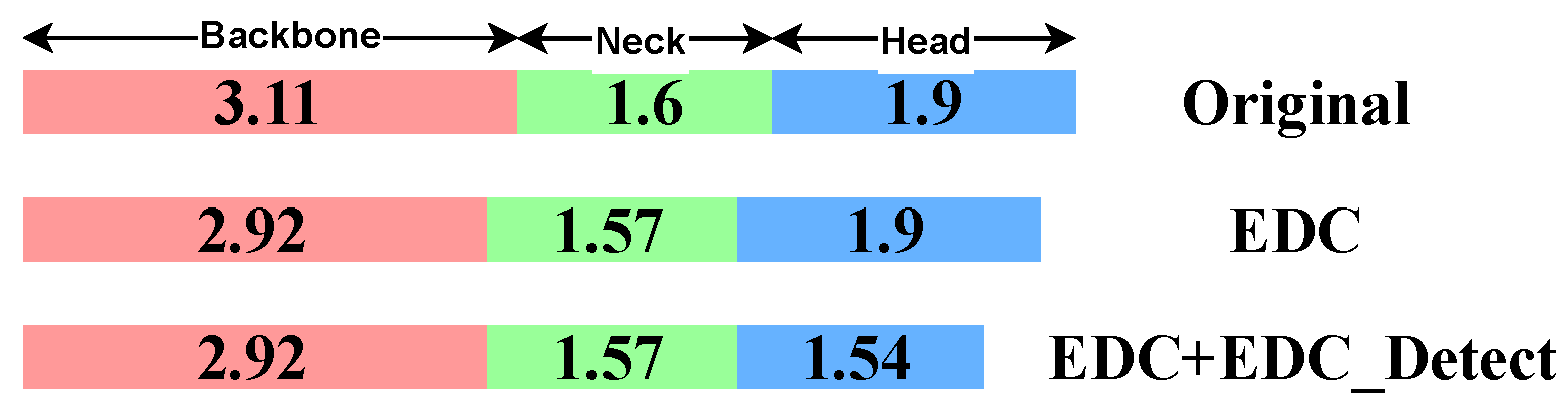
To rigorously validate the computational efficiency of the proposed module, we present a component-wise complexity analysis in Figure 6. The figure breaks down the computational cost (measured in GFLOPs) across three key network stages: backbone, neck, and head. We compare three configurations: the baseline YOLOv11 (“Original”), the model with EDC downsampling layers (“EDC”), and the fully optimized model integrating the EDC-based detection head (“EDC+EDC_Detect”).
As illustrated in the figure, the baseline model consumes 3.11 GFLOPs in the backbone. By replacing standard downsampling with our EDC module (middle row), the backbone complexity is reduced to 2.92 GFLOPs, validating the efficiency of the dual-branch compression strategy. Furthermore, the integration of the EDC_Detect module (bottom row) yields the most significant gain in the detection head, slashing its complexity from 1.9 GFLOPs to 1.54 GFLOPs. These quantitative results confirm that the EDC design effectively minimizes redundancy at every stage, collectively contributing to the lightweight nature of the Edge Aware-YOLO framework.
  • Synergy between Compression and Contextualization. The architectural flow progresses from efficient spatial compression to robust semantic expansion. While the EDC module successfully reduces computational redundancy and minimizes information loss during downsampling, the resulting feature maps require a mechanism to capture long-range dependencies and multi-scale context to ensure accurate detection. The design therefore integrates the Spatial Pyramid Shared Convolution (SPSC) immediately following the downsampling stages. This arrangement creates a critical synergy: EDC provides a lightweight, information-rich foundation, allowing the SPSC module to focus exclusively on maximizing the receptive field without the burden of processing spatially redundant data. Furthermore, by utilizing a shared-weight strategy, SPSC aligns with the parameter-saving philosophy of EDC, ensuring that the network’s depth translates into semantic richness rather than computational overhead.

3.4. Spatial Pyramid Shared Convolution (SPSC)

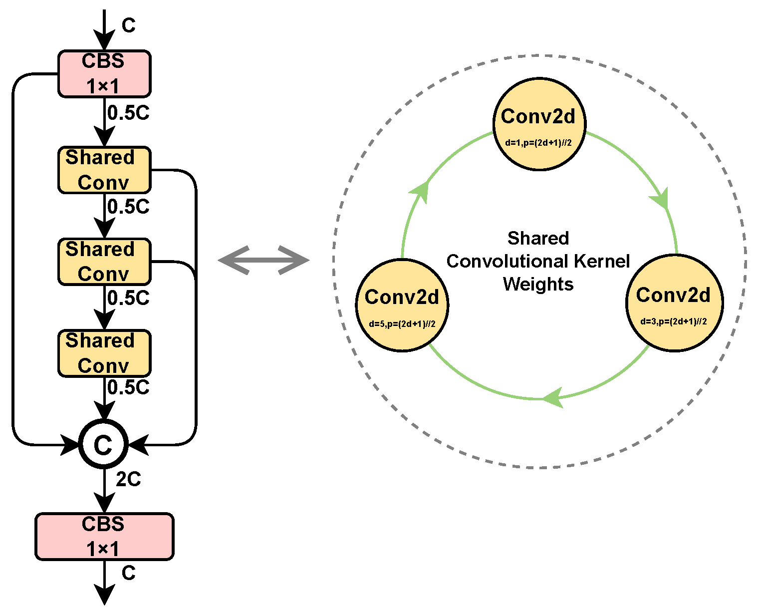
To address the issues of high-frequency detail loss from pooling operations and parameter redundancy in conventional multi-branch convolutions, we propose the Spatial Pyramid Shared Convolution (SPSC) module. This design integrates dilated convolution with a parameter sharing mechanism to achieve efficient multi-scale feature modeling.
As illustrated in Figure 7, the SPSC module constructs a spatial pyramid structure using multi-scale dilation rates ( d = 1 , 3 , 5 ) , preserving positional information by avoiding traditional pooling-based downsampling. It significantly reduces model complexity by introducing shared convolutional weights across all dilation branches—different branches reuse identical kernel parameters, The concatenation of the outputs from the dilated branches with the initial compressed feature map serves as a residual path, which maintains gradient flow and prevents feature sparsity that can arise from large dilation rates. These enhancements enable SPSC to extract fine-grained spatial details while maintaining full-resolution feature integrity.
Specifically, given an input feature map of channel dimension C, SPSC first applies a 1 × 1 CBS (Convolution-BatchNorm-SiLU) operation to compress channels from C to 0.5 C . Three parallel dilated convolution branches then operate with shared kernel weights and different dilation rates ( d = 1 , 3 , 5 ) , each adopting appropriate padding ( p = ( 2 d 1 ) / 2 ) to maintain spatial alignment. The outputs from the three branches are concatenated with the compressed input feature to form a fused representation. Subsequently, a 1 × 1 CBS layer expands the channels from the concatenated features to restore the original channel dimension C. This hierarchical process achieves efficient multi-scale feature fusion while ensuring a compact parameter footprint.
Mathematically, the output of SPSC can be formulated as
F o u t = Conv 1 × 1 ( Concat ( F c , DilatedConv ( F c , d = 1 ) , DilatedConv ( F c , d = 3 ) , DilatedConv ( F c , d = 5 ) ) )
where F c denotes the compressed feature, and all dilated convolutions share identical kernel parameters. This shared-weight spatial pyramid structure efficiently balances accuracy and efficiency, offering an enhanced receptive field without increasing model size—an essential feature for lightweight detection networks under computational constraints.

4. Experiments

In this section, we describe the experimental details (including datasets, evaluation metrics, and training procedures), discuss ablation experiments, and compare the results with existing methods.

4.1. Introduction of Datasets

In this study, five publicly available datasets were used to evaluate our model. The characteristics of these datasets are detailed in Table 1 below. The RUOD dataset is a comprehensive underwater scene dataset that covers various underwater detection challenges. It provides detailed annotations for 10 categories of underwater objects, including fish, divers, starfish, coral, sea turtles, sea urchins, sea cucumbers, scallops, squid, and jellyfish.
The SVRDD dataset focuses on road surface defect detection, containing six defect categories and one easily confused non-concrete pavement type. These include longitudinal cracks, transverse cracks, alligator cracks, potholes, longitudinal repairs, transverse repairs, and manhole covers. The dataset features diverse backgrounds, including pedestrians, vehicles, buildings, overpasses, trees, and their shadows, captured under various conditions such as different seasons, weather, and lighting.
The SHWD dataset is designed for safety helmet wearing and head detection, comprising 7581 images with annotations for 9044 helmet wearing objects (positive) and 111,514 non-helmet-wearing head objects (negative).
The VOC dataset is the official dataset for the PASCAL VOC challenge, containing 20 object categories. Each image is meticulously annotated, covering categories such as people, animals (e.g., cats, dogs, birds), vehicles (e.g., cars, boats, airplanes), and furniture (e.g., chairs, tables, sofas). On average, each image contains 2.4 objects, and all annotated images include labels required for object detection.
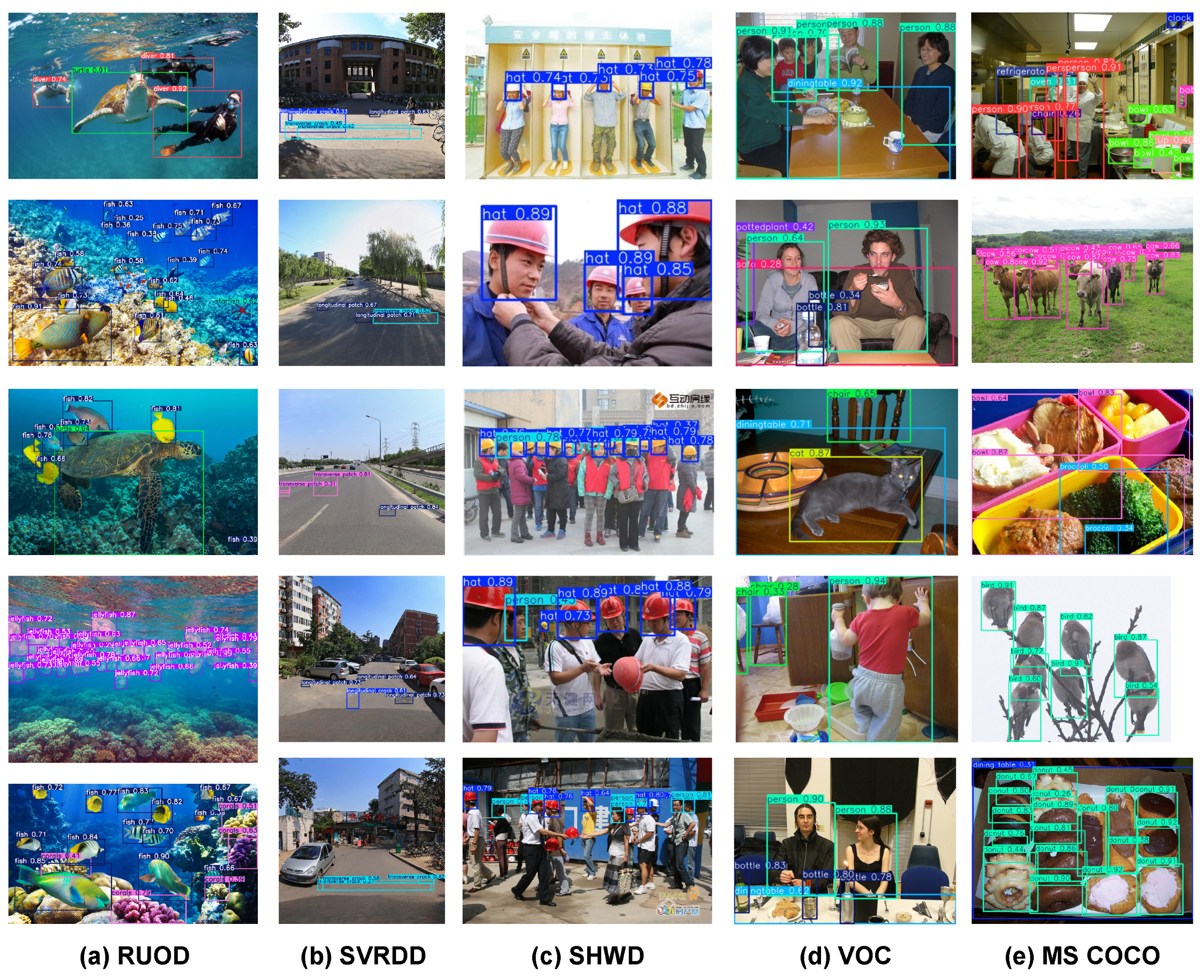
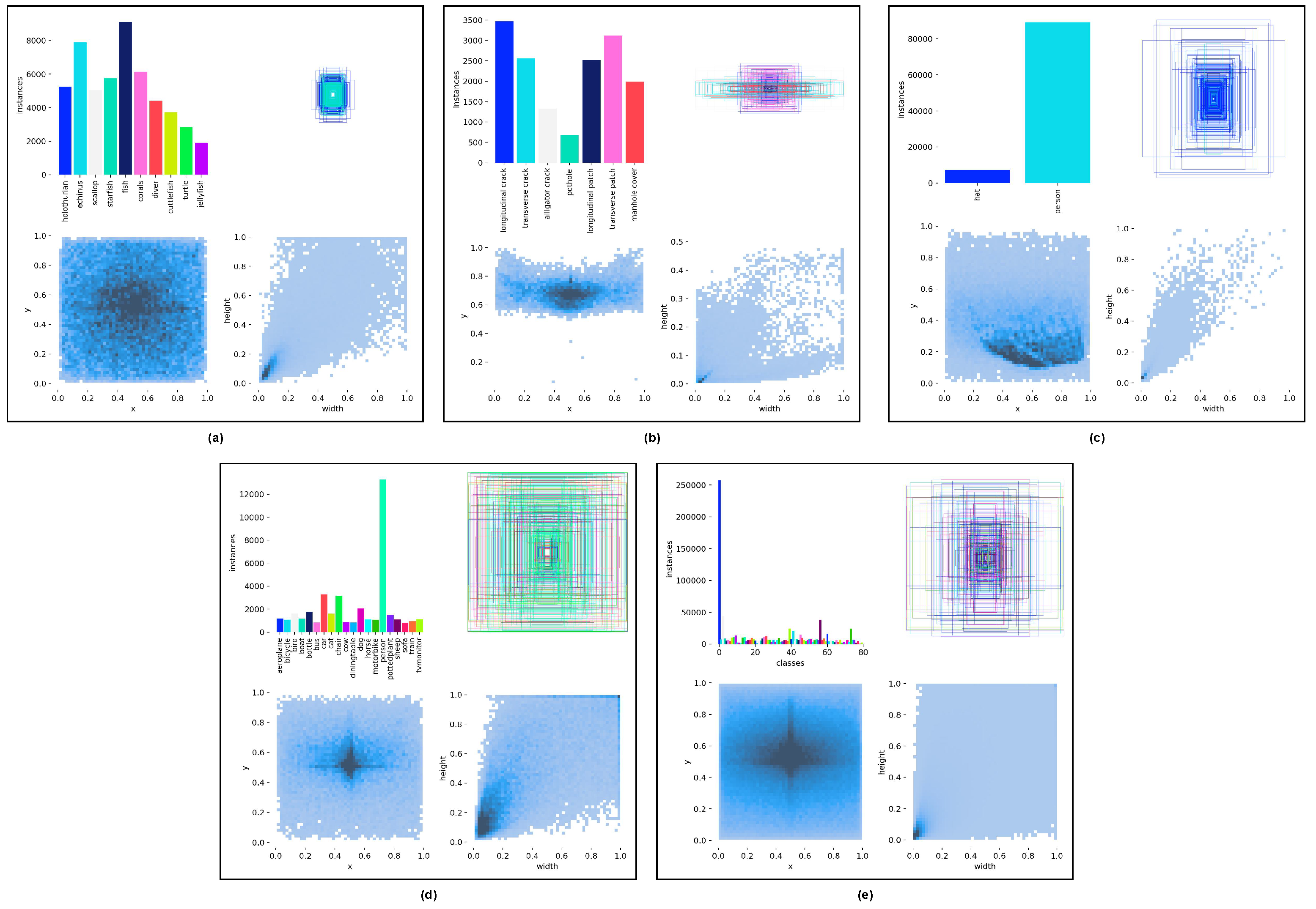
The MSCOCO dataset, constructed by Microsoft, is large-scale, containing over 330,000 images, with more than 200,000 images being meticulously annotated. Figure 8 showcases some images from these five datasets. Figure 9 shows the characteristics of each dataset. The upper left corner displays a histogram of the frequency of each category appearing in the training set, which helps to understand the distribution of different categories in the dataset; Set the center point coordinates of all bounding boxes at the same position in the upper right corner to observe the width to height ratio of each label box in each training sample. This approach can reveal the diversity of object sizes and shapes in the dataset, helping to identify potential data imbalances or outliers; Draw a histogram of the x and y coordinate variables at the bottom left corner to display the distribution of these coordinates in the dataset. This type of chart can help us understand the distribution pattern of the target object in the image, such as whether certain regions are more commonly associated with specific types of objects; Display histograms of width and height variables in the lower right corner to show the aspect ratio of the target in the dataset relative to the entire image.

4.2. Evaluation Indicators

We adopt mean average precision (mAP) as the primary metric for evaluating model accuracy, with precision (P) and recall (R) as supplementary metrics. These metrics are expressed as follows:
Precision = TP TP + FP
Recall = TP TP + FN
AP = 0 1 p ( r ) d r
mAP = 1 n i = 1 n AP i
where TP is a positive sample judged as a positive sample by the model; FP means a negative sample is judged as a positive sample; FN means a positive sample is judged as a negative sample; p ( r ) represents the precision as a function of recall, and n is the number of a certain category; AP i is the detection accuracy of category i. Specifically, mAP50 and mAP50-95 are calculated at intersection over union (IoU) thresholds of 0.5 and from 0.5 to 0.95 with a step size of 0.05, respectively. Additionally, we use Params (M) and floating point operations (FLOPs) to evaluate the model’s size and computational complexity.

4.3. Experimental Environments

All training and inference are performed on a Windows 11 system equipped with a single NVIDIA RTX 4060Ti GPU. The software environment includes CUDA 12.1, Python 3.11, and PyTorch 2.2.
For a fair comparison, we adopt a common training strategy across all experiments. The models are trained for 200 epochs using the AdamW optimizer with a learning rate of 0.0004, β of [0.9, 0.999], and a weight decay of 0.0001. We use a batch size of 4. Unless otherwise specified, all other settings follow the common practices used in state-of-the-art detectors. The computational cost is measured in GFLOPs at the same 640 × 640 input resolution.

4.4. Comparative Experiments on VSCIB

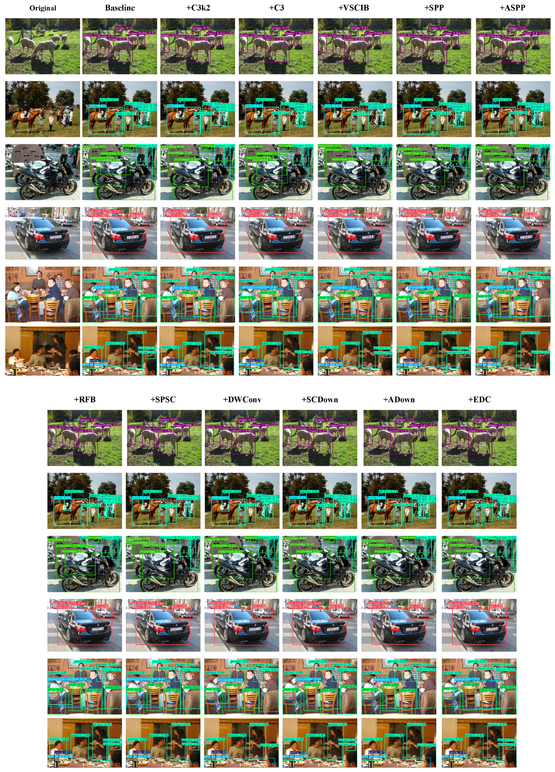
As shown in Figure 10, +VSCIB’s core advantages over +C3k2, +C2f, and +C3 manifest in complex scenarios through superior contour adherence and anti-interference capability. In sheep occlusion scenarios, +VSCIB’s detection boxes tightly adhere to animal limb edges, while +C3k2/+C3 exhibit box fragmentation or over-extension in occluded areas. For motorcycle metal part reflections and indoor dining table small objects, +VSCIB preserves complete detection boxes in headlight reflection zones and tableware edges through saliency-weighted high-frequency feature enhancement, whereas +C2f loses texture details due to lightweight design (e.g., misclassifying motorcycle handle grids as background).
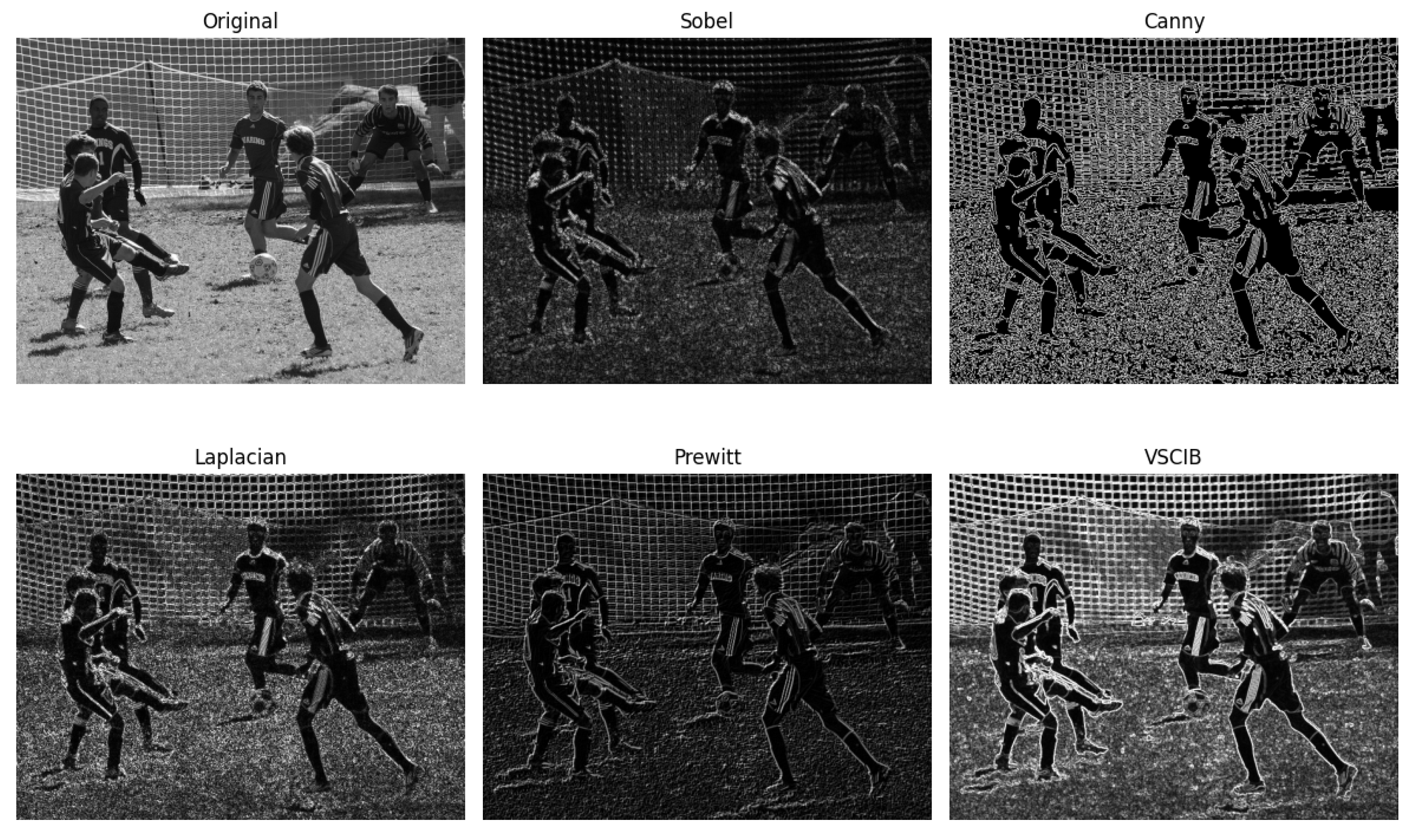
As shown in Figure 11, the proposed VSCIB module demonstrates superior edge feature extraction capabilities compared to classical operators. Sobel, Canny, and Laplacian operators generate fragmented edge contours with high noise sensitivity (e.g., incomplete jersey boundaries in soccer player images), whereas VSCIB produces continuous and semantically meaningful edges. Notably, VSCIB preserves fine-grained details like grass texture in the soccer field and the grid structure of the goal net, which are partially lost in Prewitt and Laplacian outputs.
Table 2 validates the balanced performance–efficiency trade-off of VSCIB in the YOLOv11 framework. Despite maintaining a compact architecture (5.5 MB model size, 2.6M parameters), VSCIB achieves state-of-the-art metrics: 80.9% precision (+0.5% vs. C3k2), 74.8% recall (+0.8% vs. C3k2), and 62.7% mAP50-95 (+3.3% vs. C2f). The computational cost (6.6 GFLOPs) remains comparable to lightweight counterparts like C3k2 (6.5 GFLOPs), demonstrating minimal overhead from the proposed dynamic kernel adaptation mechanism.

4.5. Comparative Experiments on EDC

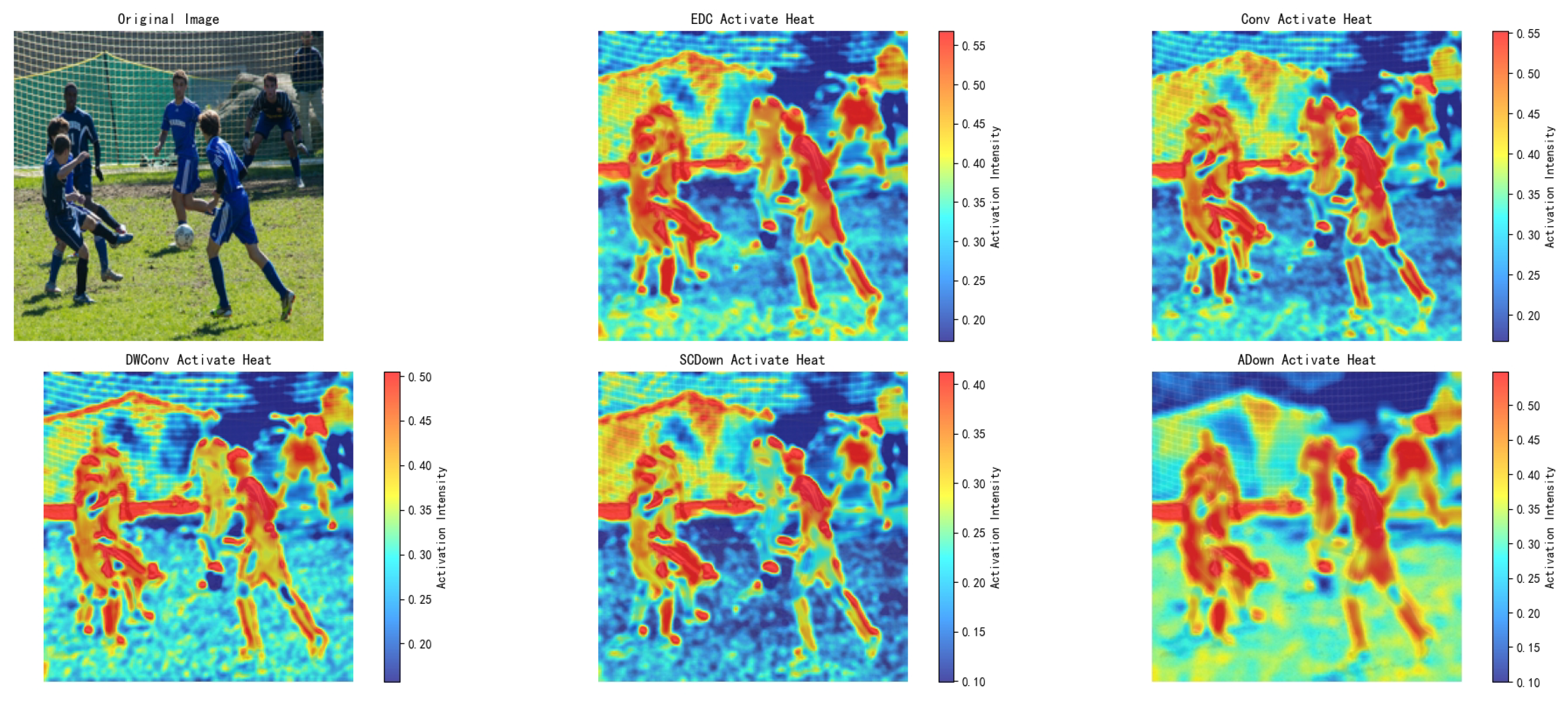
As shown in Figure 10, +ADown and +DWConv are prone to bounding box offset in the scene; compared with +EDC, +ADown has experienced multiple missed detections; compared to +Conv, +EDC can better detect the geometric features of the detection box and object.As shown in Figure 12, significant responses are produced in both the athlete’s full body posture and the background area of the goal. Conv and EDC have similar response effects, but there is edge blurring in the limb contact area; DWConv has discontinuous response to details; SCDond exhibits abnormal activation overheating in the trunk area; Adown suffers from significant loss of texture details.
As shown in Table 3, while maintaining high accuracy (mAP50 81.4% is on par with standard Conv), the recall rate (75.1%) is significantly ahead (1.4% higher than DWConv), and the overall detection performance (mAP50-95 61.8%) is optimal. Its model size (4.6 MB) and computational complexity (5.7 GFLOPs) are also relatively good.

4.6. Comparative Experiments on SPSC

As shown in Figure 10, we integrated the module into YOLOv11 and compared the detection performance of different modules on the VOC dataset; in crowded pedestrian scenarios, +SPSC preserves high-frequency details like limb joints, whereas +RFB exhibits extensive bounding box overlaps and SPPF shows boundary over-extension. For vehicle detection, +SPSC tightly confines detection boxes to metallic body regions, while +ASPP introduces false positives from road cracks and +SPPF produces blurred car rear contours.
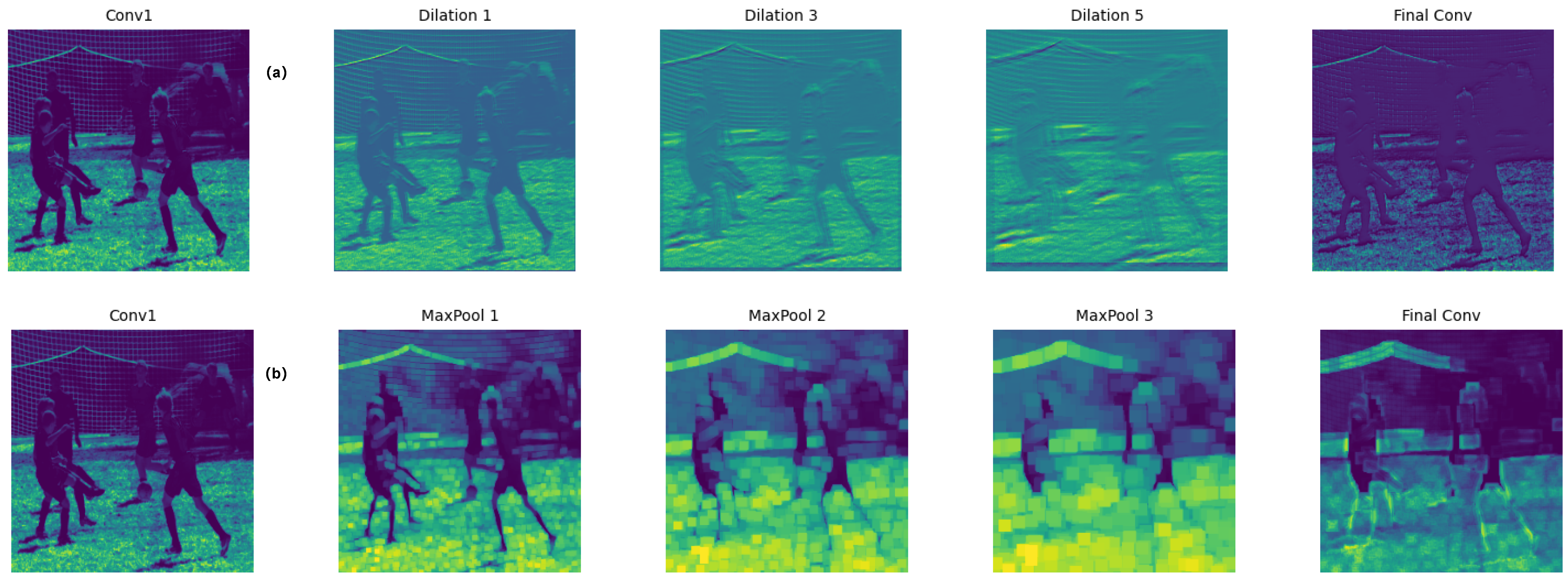
Figure 13 demonstrates the differences between SPSC and SPPF in intermediate feature maps. SPSC expands receptive fields through dilated convolution while maintaining resolution, whereas SPPF progressively compresses spatial information via pooling operations. By comparing color patterns, resolution levels, and activation distributions in the feature maps, their distinct approaches to feature extraction and information preservation can be visually discerned.
Table 4 demonstrates SPSC’s comprehensive advantages on YOLOv11. Its recall rate (75.4%) is significantly higher than other modules (e.g., 74.4% for SPPF), benefiting from dilated convolution’s detail preservation capability. The mAP50-95 (62.6%) outperforms RFB (62.1%), while computational efficiency (6.5 GFLOPs) outperforms ASPP (8.1 GFLOPs). This achieves optimal balance between model size (5.8MB) and computational load.

4.7. Comparisons Experiments on Other Models

As detailed in Table 5, to validate the effectiveness of the proposed modules, we conducted comprehensive experiments on multiple public datasets. The results demonstrate that Edge Aware-YOLO significantly outperforms current mainstream models in both detection accuracy and computational efficiency. Specifically, on the RUOD dataset, our model achieves 85.8% mAP50 and 68.4% mAP50-95 (representing gains of 1.1% and 1.0% over YOLOv8n), while simultaneously slashing computational cost by 2.9 GFLOPs. Similarly, on the MS COCO dataset, it surpasses advanced models like YOLOv11 with scores of 56.3% and 40.5%. Notably, compared to heavyweight detectors such as Faster R-CNN, Edge Aware-YOLO reduces parameter count and computational load by over 94% and 90%, respectively, proving its superiority in resource-constrained tasks.
In summary, the innovative modules proposed in this paper, through dynamic edge extraction (VSCIB), optimized multi-scale feature fusion (SPSC), and efficient downsampling (EDC), effectively address the bottlenecks of performance and cost in complex scenarios. The Edge Aware-YOLO model not only sets a new benchmark for detection accuracy but also ensures exceptional computational efficiency, providing a reliable solution for real-time tasks. Future work will explore deploying these modules in more diverse environments and further optimizing inference speed.

4.8. Ablation Study and Synergy Analysis

To comprehensively evaluate the contribution of each module and validate the systemic design logic, we conducted a series of ablation experiments on the VOC2007+2012 dataset. These experiments were designed not only to test individual components but to verify the synergistic effects between the VSCIB, SPSC, and EDC modules.

4.8.1. Logic of Module Synergy

Before analyzing the quantitative results, it is essential to clarify the rationale behind the integration of these specific modules. We constructed the framework as a cohesive system to address the trade-off between edge perception and computational efficiency:
1.
Complementary Perception (VSCIB + SPSC): The VSCIB acts as a front-end feature enhancer, explicitly capturing high-frequency edge details. Since standard pooling layers tend to discard these fragile features, the SPSC serves as a mid-stage preserver. By replacing pooling with shared dilated convolutions, SPSC expands the receptive field while explicitly preserving the sharp edge features extracted by VSCIB, ensuring geometric priors are propagated to the detection head.
2.
Efficiency–Accuracy Trade-off (EDC + VSCIB): The rotatable kernels in VSCIB inevitably incur computational costs. To counterbalance this, the EDC acts as a global efficiency regulator. Using a lightweight dual-branch architecture for downsampling, EDC significantly reduces the parameter count and GFLOPs in the backbone and head. This creates a “computational budget” that allows us to afford the sophisticated VSCIB module without compromising real-time performance.
3.
Holistic Optimization: The combination aims for a non-linear performance boost where EDC enables the speed, VSCIB provides the precision, and SPSC ensures feature integrity across scales.

4.8.2. Quantitative Analysis

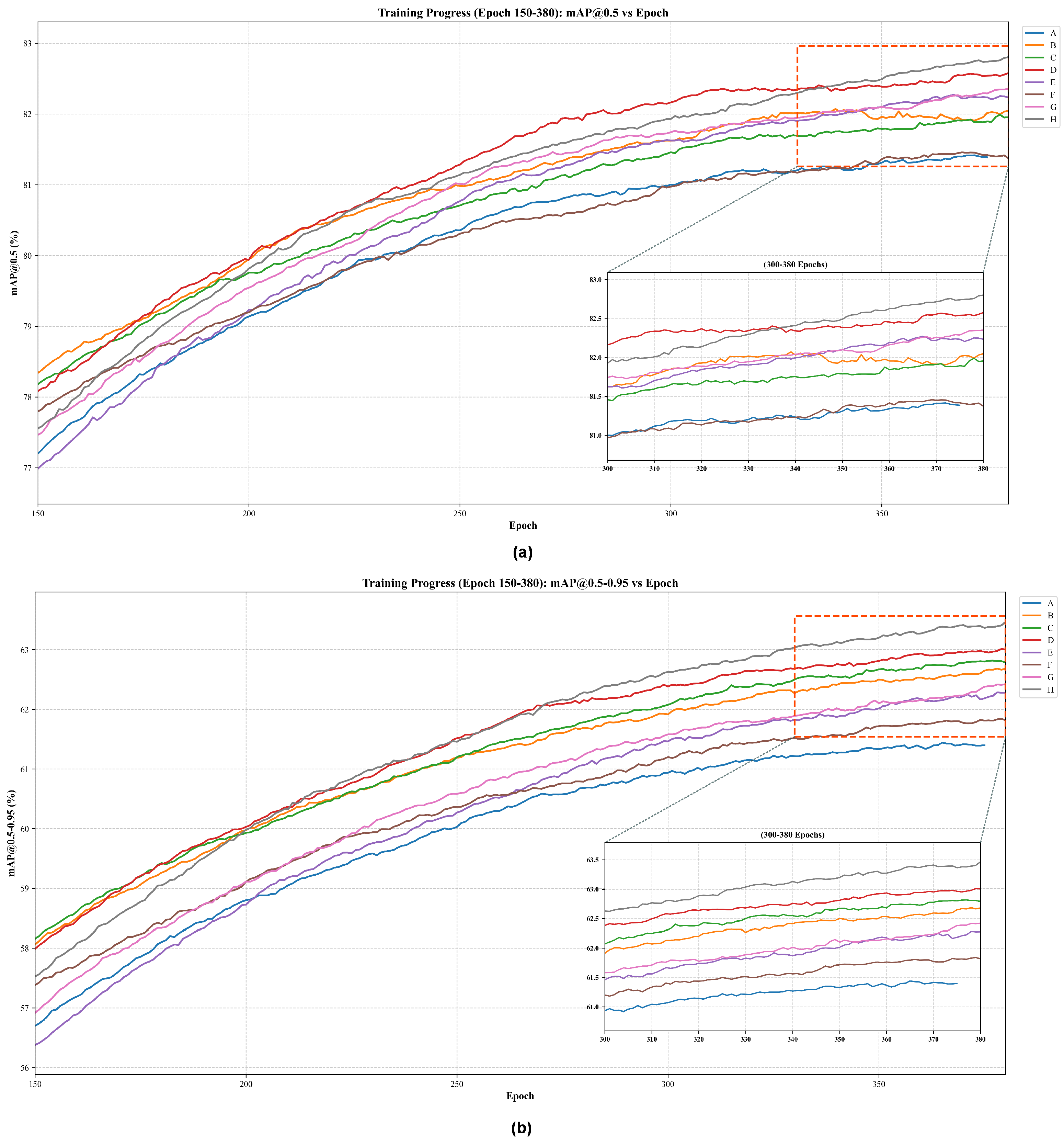
Guided by this design logic, we evaluated the models as detailed in Table 6 and Figure 14. The Baseline model (Experiment A), without any added modules, achieves 81.4% mAP50 and 61.4% mAP50-95 with 2.5M parameters and 6.5 GFLOPs.
Individual Contributions: When the VSCIB module is added individually (Experiment B), detection accuracy improves to 82.0% mAP50 and 62.7% mAP50-95. However, this comes with a slight increase in computational cost (6.6 GFLOPs), confirming its role as a high-precision but cost-intensive feature extractor. Conversely, the EDC module alone (Experiment F) significantly reduces model size (2.2M parameters) and complexity (5.7 GFLOPs) but yields limited accuracy gains (81.5% mAP50). This validates EDC’s primary role as an efficiency optimizer rather than a direct performance booster. The SPSC module (Experiment G) performs exceptionally well in isolation, achieving 82.5% mAP50, demonstrating its effectiveness in multi-scale feature aggregation.
Synergistic Effects: The true value of our framework is revealed in the combined experiments. When EDC is paired with VSCIB (Experiment C), the model achieves higher accuracy (82.1% mAP50) than the baseline while maintaining lower computational costs (5.8 GFLOPs), proving that EDC successfully offsets the overhead of VSCIB. Furthermore, the combination of VSCIB and SPSC (Experiment D) pushes the mAP50-95 to 63.2%, verifying the “Extract-and-Preserve” hypothesis.
Finally, the full integration of VSCIB, EDC, and SPSC (Experiment H) delivers the optimal performance: 83.2% mAP50 and 63.9% mAP50-95, representing a substantial gain over the baseline. Crucially, this is achieved with only 2.4M parameters and 5.8 GFLOPs—lower than the original YOLOv11n. This conclusive result confirms that the synergistic interaction of the three modules simultaneously enhances detection accuracy and computational efficiency, achieving the paper’s core design objective.
The inclusion of FPS metrics in Table 6 highlights the efficiency trade-off mechanism designed in our framework. While adding the VSCIB module alone (Experiment B) reduces the inference speed from 115 FPS to 105 FPS due to the computational overhead of dynamic kernels, the integration of the EDC module (Experiment F) significantly boosts speed to 132 FPS by reducing feature map redundancy. Consequently, our final model (Experiment H) achieves a balanced speed of 119 FPS, which is slightly faster than the baseline (115 FPS). This empirically proves that the lightweight design of EDC successfully compensates for the complexity of VSCIB, delivering a model that is both more accurate and computationally efficient suitable for real-time applications.

4.9. Qualitative Analysis

To systematically understand how edge features influence detection performance, we analyze the model’s behavior through confusion matrices, detection bounding boxes, and attention heatmaps.
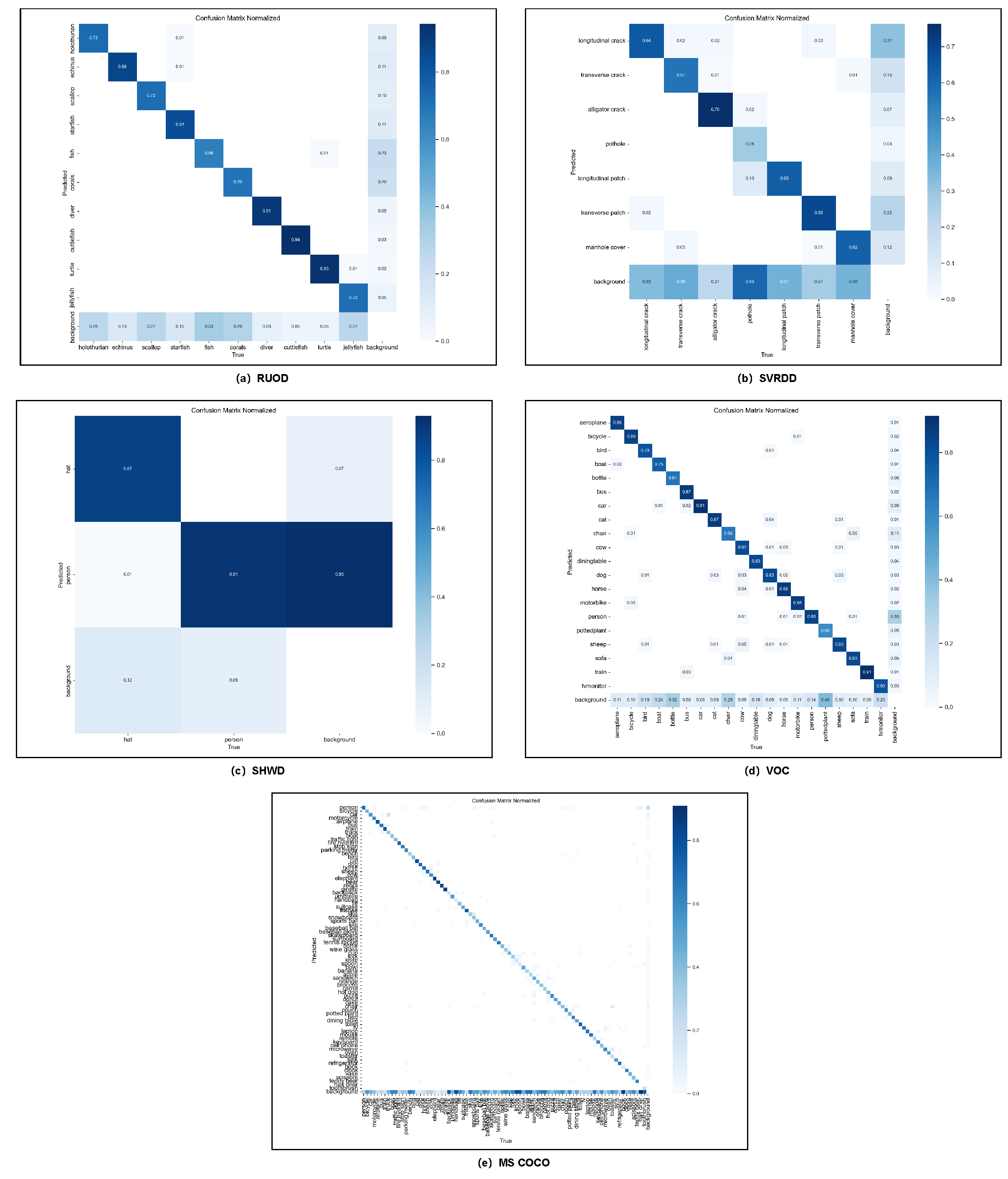
Classification Precision: As shown in Figure 15, the confusion matrix indicates high diagonal values with minimal off-diagonal noise. This suggests that the edge features serve as discriminative geometric signatures, helping the model distinguish between visually similar categories (e.g., distinguishing pavement cracks from manhole covers) by capturing their unique contour topologies.
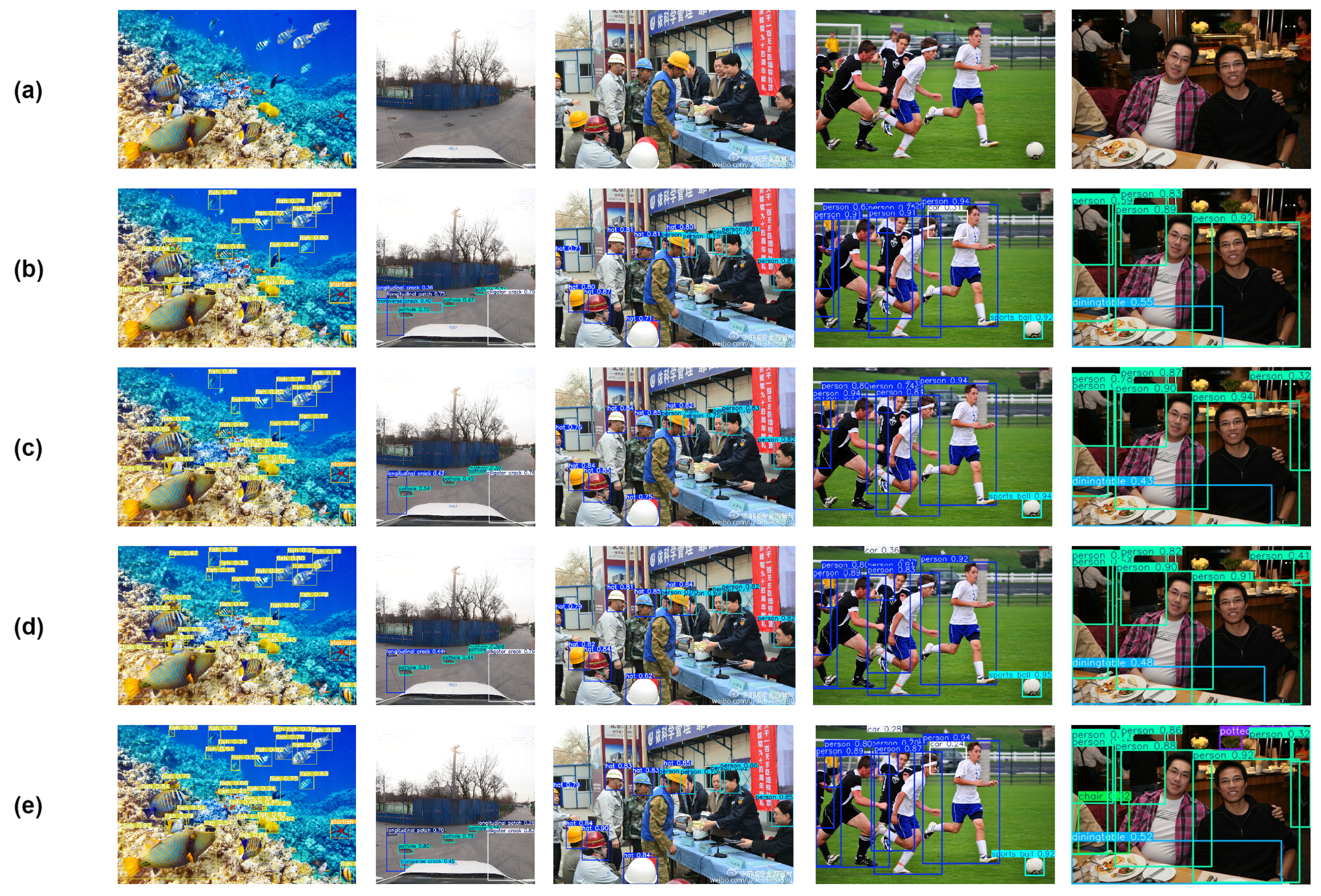
Localization and Boundary Adherence (Figure 16): The direct impact of edge features on localization is evident in the comparison of bounding boxes. Standard models (e.g., YOLOv8n, YOLOv11n) often produce “loose” bounding boxes that include background areas or fail to separate overlapping objects. In contrast, Edge Aware-YOLO exhibits superior boundary adherence. For instance, in the coral reef scene (Figure 16, Row 1), the fish outlines are faint against the background. The VSCIB module, by explicitly calculating multi-directional gradients, sensitizes the network to these subtle transitions. This allows our model to generate bounding boxes that tightly wrap around the irregular shapes of the fish, rather than merely framing the general area. This confirms that edge information acts as a fine-grained guide for regression branches, improving IoU accuracy.
Attention Mechanism and Noise Suppression (Figure 17):
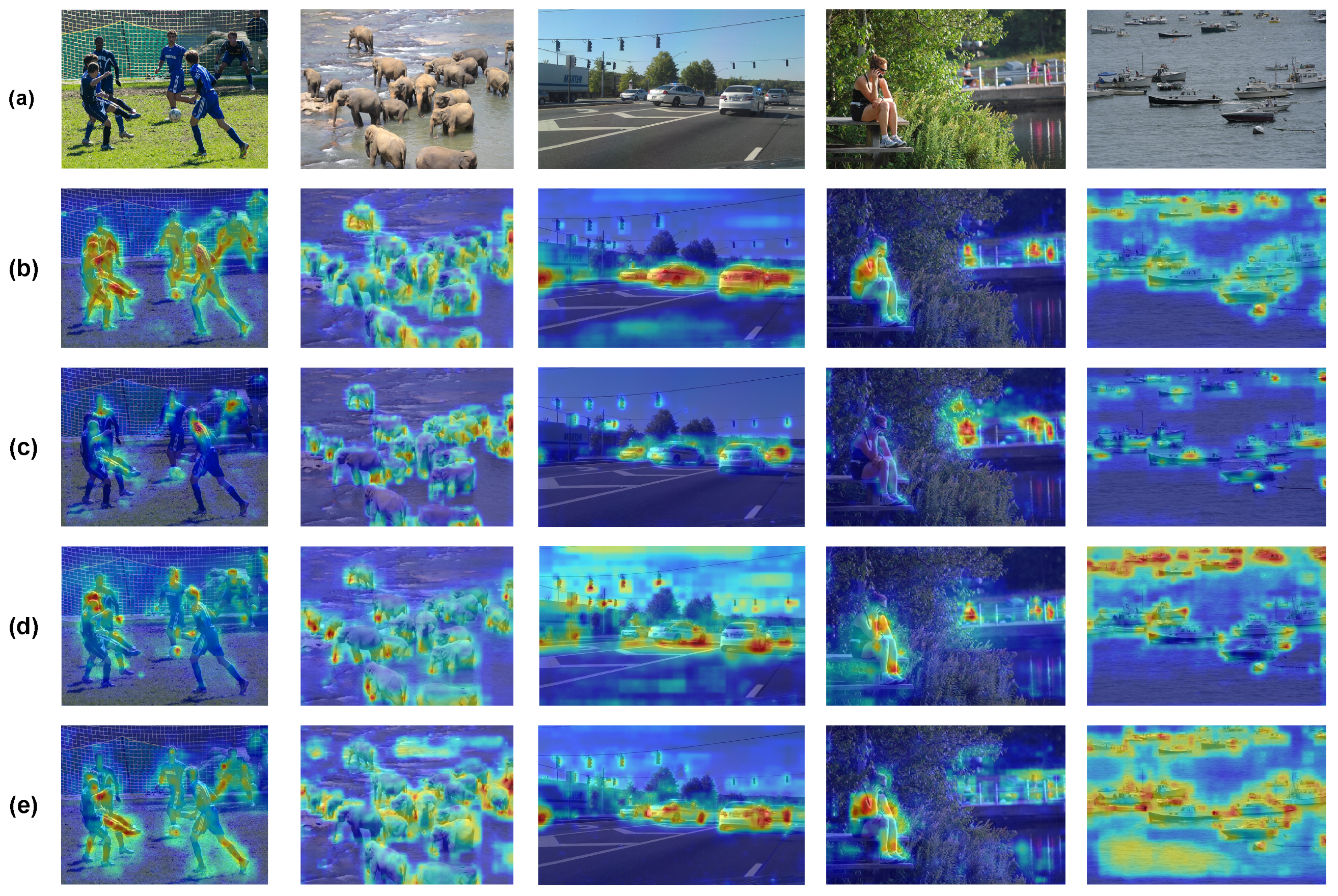
The Grad-CAM heatmaps provide the most direct evidence of how edge features modulate feature extraction.
1.
Spatial Constraint: In the baseline heatmaps (Columns c-e), activation regions are diffuse and often “spill over” into the background. This indicates that standard convolutions rely heavily on texture correlations, which are continuous across boundaries.
2.
Edge Guidance: In contrast, our model’s heatmaps (Column b) display sharp cutoffs at object boundaries. For example, on the diver’s body, the high activation strictly follows the limb edges. This phenomenon demonstrates that the VSCIB module effectively introduces a geometric constraint: the strong gradient response at the edges acts as a barrier, confining the semantic features within the object’s instance mask.
3.
Background Suppression: By prioritizing structural edges over textural noise, the model effectively suppresses irrelevant background activations. This is crucial in complex scenes where background textures (e.g., water ripples or street lights) often trigger false positives in baseline models.
In summary, the explicit modeling of edge features affects detection results by transforming diffuse semantic attention into geometrically constrained focal points, thereby enhancing both localization precision and resistance to background interference.
Figure 17. GradCAM generates visual results using different models. (a) Original, (b) Ours, (c) YOLOv8n, (d) YOLOv10n, (e) YOLO11.The heatmap uses a standard red-to-blue color scale, where red highlights regions of high activation (strong model attention) and blue indicates low activation.
Electronics 15 00449 g017

4.10. Robustness Analysis in Extreme Scenarios

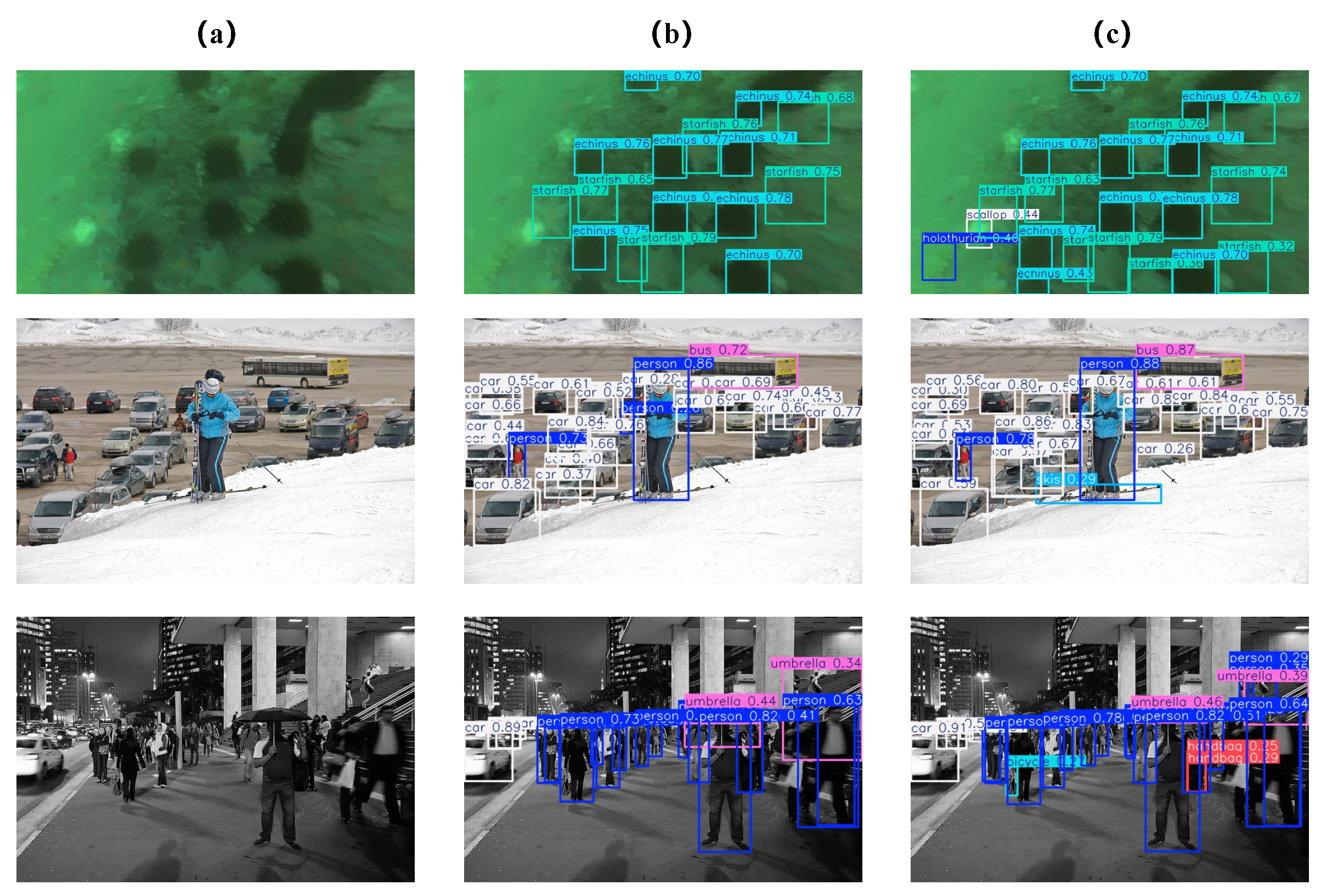
To address concerns regarding performance under severe edge degradation, we evaluated the model in extreme conditions: motion blur (Row 1), background clutter (Row 2), and low lighting with occlusion (Row 3). As shown in Figure 18, our method (Column c) consistently outperforms the baseline (Column b):
1.
Severe Blur (Row 1): The baseline does not detect the holothurian due to diffuse gradients in the turbid water. Our method successfully localizes it, validating that VSCIB’s explicit geometric prior captures faint edges better than implicit adaptive methods.
2.
Background Clutter (Row 2): In the snowy scene, the baseline misses the fine-grained skis. Our model, utilizing VSCIB’s multi-directional perception, accurately isolates the thin, elongated structure from the chaotic background.
3.
Low Lighting and Occlusion (Row 3): The baseline misses the bicycle and the handbag (red box) in the dark street. Our method recovers these targets, attributed to the synergy of VSCIB’s noise suppression ( S m operator) and SPSC’s expanded contextual receptive field.
These results empirically confirm that Edge Aware-YOLO maintains high robustness even when visual features are significantly degraded.
Figure 18. Detection results in extreme scenarios. (a) Original, (b) Baseline, (c) Ours. Row 1: Our method detects the blurred “holothurian”. Row 2: Our method identifies the “skis” in clutter. Row 3: Our method recovers the “bicycle” and “handbag” (red box) in low-light occlusion.
Electronics 15 00449 g018

5. Discussion

In this study, we propose an innovative object detection framework—Edge Aware-YOLO—aimed at addressing three key challenges in complex environments: precise extraction of dynamic edge features, efficient fusion of multi-scale information, and optimization of model computational efficiency. Specifically, (1) Edge Aware-YOLO introduces the Variable Sobel Compact Inverted Block (VSCIB), which adaptively adjusts the size and orientation of convolutional kernels, significantly enhancing the model’s perception of complex edge features; (2) through the Spatial Pyramid Shared Convolution (SPSC) module, it replaces traditional pooling operations with shared convolutional kernels and dilated convolutions, achieving efficient multi-scale feature fusion while reducing computational overhead; and (3) the Efficient Downsampling Convolution (EDC) module combines downsampling with semantic refinement branches, maximizing the retention of critical information while reducing computational load. The synergistic effect of these modules enables Edge Aware-YOLO to excel in degraded scenarios while maintaining high inference speed.

5.1. Performance and Generalizability

Experimental results demonstrate that Edge Aware-YOLO significantly outperforms current mainstream models on multiple public datasets. For example, on the RUOD dataset, Edge Aware-YOLO achieves an mAP50 of 85.8%, which is 1.1 percentage points higher than YOLOv8n, while reducing computational cost by 2.9 GFLOPs. On the MS COCO dataset, Edge Aware-YOLO achieves mAP50 and mAP50-95 of 56.3% and 40.5%, respectively, surpassing advanced models such as YOLOv11. Additionally, Edge Aware-YOLO maintains low parameter (2.4M) and computational (5.8 GFLOPs) costs, significantly outperforming traditional detection models (e.g., Faster R-CNN) and other lightweight models.
It is worth noting that while this study implements the proposed modules within the YOLOv11 framework, they are designed as general components rather than architecture-specific bindings. Specifically, the VSCIB can conceptually replace standard convolutional layers in any CNN backbone (e.g., ResNet or VGG) to enhance edge sensitivity; the EDC serves as a generic efficient downsampling unit; and the SPSC can be integrated into the neck of various single-stage or two-stage detectors. We selected the YOLO architecture as the primary testbed because it represents the state-of-the-art in real-time detection, imposing the strictest constraints on parameter efficiency.

5.2. Theoretical Comparisons

While attention-based mechanisms (e.g., CBAM, SE) and Transformer architectures (e.g., RT-DETR) have set new benchmarks in global feature aggregation, our Edge Aware-YOLO offers distinct advantages in specific degraded scenarios:
1.
Boundary Ambiguity: Attention mechanisms rely on implicit feature matching. In scenarios with severe motion blur or low contrast (e.g., turbid underwater scenes), feature correlations become weak, often leading to “oversmoothed” boundaries. In contrast, our VSCIB module introduces an explicit geometric prior via rotatable Sobel operators. This imposes a structural constraint that forces the network to lock onto high-frequency gradient changes, offering superior boundary adherence where learned attention maps might fail to converge.
2.
Occlusion Handling: Transformers excel at handling occlusion via global self-attention but suffer from quadratic computational cost ( O ( N 2 ) ). Our framework addresses occlusion through the SPSC module, which employs dilated convolutions to expand the receptive field. This allows the model to capture sufficient surrounding context to infer occluded objects with linear complexity ( O ( N ) ), achieving a pragmatic balance between contextual robustness and real-time latency.

5.3. Limitations and Failure Case Analysis

Despite its outstanding performance, it is necessary to rigorously discuss the boundaries of our method’s effectiveness, particularly concerning noise robustness and failure cases.
  • Sensitivity to Adversarial Perturbations. While our method demonstrates strong robustness against natural environmental noise (e.g., underwater turbidity, low-light ISO noise) due to the smoothing operator S m in VSCIB, its resilience against adversarial attacks remains an open research question. Unlike random natural noise, adversarial perturbations are often meticulously calculated to invert gradient directions with imperceptible texture changes. Since VSCIB explicitly relies on gradient computation, it may be theoretically more susceptible to such gradient-targeted attacks than purely semantic-based networks. We acknowledge that no specific adversarial defense mechanisms (e.g., adversarial training) were integrated into this study.
    Failure Cases in High-Frequency Textures. Although the VSCIB includes a low-pass filtering mechanism to suppress noise, it may encounter difficulties in scenarios with extremely dense, high-frequency repetitive patterns (e.g., dense rain streaks, camouflage nets, or chain-link fences). In these cases, the texture frequency may overlap with the edge frequency of the target objects. If the texture intensity is strong, the Sobel operators might interpret these patterns as structural edges, leading to false positives or fragmented detection boxes. Future iterations will need to explore adaptive frequency-domain filtering to better distinguish between structural edges and high-frequency textural noise.

5.4. Future Work

Based on the identified limitations and the current results, future research will focus on the following:
1.
Adversarial Robustness: Investigating the integration of adversarial training strategies to fortify the edge-aware mechanisms against synthetic perturbations and gradient-based attacks.
2.
Architecture Optimization: Combining Neural Architecture Search (NAS) to further reduce computational complexity and parameters.
3.
Model Compression: Exploring pruning and quantization for deployment on extreme edge devices (e.g., mobile or embedded systems).
4.
Cross-Domain Adaptability: Validating the generalization ability of Edge Aware-YOLO in other domains where edge features are critical, such as medical image analysis (e.g., lesion segmentation) and remote sensing.
5.
Integration with Heterogeneous Architectures: Extending the application of the proposed modules (VSCIB, EDC, SPSC) beyond the YOLO framework to other mainstream backbones (e.g., ResNet, Swin Transformer) and detection heads (e.g., Faster R-CNN, RetinaNet) to comprehensively verify their architectural universality and plug-and-play capability.
Through continuous research, we believe that Edge Aware-YOLO will provide an efficient solution for object detection in complex scenarios, balancing the rigorous demands of theoretical robustness and engineering efficiency.

Author Contributions

Conceptualization, X.P. and J.L.; methodology, X.P.; software, X.P. and K.X.; validation, X.P. and K.X.; formal analysis, X.P.; investigation, X.P.; resources, J.L.; data curation, X.P.; writing—original draft preparation, X.P.; writing—review and editing, J.L.; visualization, X.P.; supervision, J.L.; project administration, J.L.; funding acquisition, J.L. All authors have read and agreed to the published version of the manuscript.

Funding

This research was funded by the Central South University of Forestry and Technology Graduate Student Science and Technology Innovation Fund, grant number 2023CX02094, and the National Program on Key Research during the Fourteenth Five-Year Plan Period, grant number 2022YFD2200505.

Data Availability Statement

All datasets used are publicly available.

Acknowledgments

The authors would like to thank the Central South University of Forestry and Technology for providing the experimental environment and computing resources. We also extend our gratitude to the anonymous reviewers for their constructive comments and suggestions that helped improve the quality of this manuscript.

Conflicts of Interest

The authors declare no conflicts of interest.

References

  1. Bogdoll, D.; Nitsche, M.; Zöllner, J.M. Anomaly detection in autonomous driving: A survey. In Proceedings of the IEEE/CVF Conference on Computer Vision and Pattern Recognition, New Orleans, LA, USA, 19–20 June 2022; pp. 4488–4499. [Google Scholar]
  2. Dos Reis, D.H.; Welfer, D.; De Souza Leite Cuadros, M.A.; Gamarra, D.F.T. Mobile robot navigation using an object recognition software with RGBD images and the YOLO algorithm. Appl. Artif. Intell. 2019, 33, 1290–1305. [Google Scholar] [CrossRef]
  3. Zeng, F.; Dong, B.; Zhang, Y.; Wang, T.; Zhang, X.; Wei, Y. Motr: End-to-end multiple-object tracking with transformer. In Computer Vision—ECCV 2022; Springer: Cham, Switzerland, 2022; pp. 659–675. [Google Scholar]
  4. Girshick, R. Fast r-cnn. In Proceedings of the the IEEE International Conference on Computer Vision, Santiago, Chile, 7–13 December 2015; pp. 1440–1448. [Google Scholar]
  5. He, K.; Gkioxari, G.; Dollár, P.; Girshick, R. Mask r-cnn. In Proceedings of the IEEE International Conference on Computer Vision, Venice, Italy, 22–29 October 2017; pp. 2961–2969. [Google Scholar]
  6. Tian, Z.; Shen, C.; Chen, H.; He, T. FCOS: A simple and strong anchor-free object detector. IEEE Trans. Pattern Anal. Mach. Intell. 2020, 44, 1922–1933. [Google Scholar] [CrossRef] [PubMed]
  7. Wang, C.; He, W.; Nie, Y.; Guo, J.; Liu, C.; Wang, Y.; Han, K. Gold-YOLO: Efficient object detector via gather-and-distribute mechanism. In Advances in Neural Information Processing Systems; MIT Press: Cambridge, MA, USA, 2023; Volume 36, pp. 51094–51112. [Google Scholar]
  8. Xu, X.; Jiang, Y.; Chen, W.; Huang, Y.; Zhang, Y.; Sun, X. Damo-yolo: A report on real-time object detection design. arXiv 2022, arXiv:2211.15444. [Google Scholar]
  9. Bochkovskiy, A.; Wang, C.Y.; Liao, H.Y.M. Yolov4: Optimal speed and accuracy of object detection. arXiv 2020, arXiv:2004.10934. [Google Scholar] [CrossRef]
  10. Li, C.; Li, L.; Geng, Y.; Jiang, H.; Cheng, M.; Zhang, B.; Ke, Z.; Xu, X.; Chu, X. Yolov6 v3. 0: A full-scale reloading. arXiv 2023, arXiv:2301.05586. [Google Scholar]
  11. Dai, J.; Qi, H.; Xiong, Y.; Li, Y.; Zhang, G.; Hu, H.; Wei, Y. Deformable convolutional networks. In Proceedings of the IEEE International Conference on Computer Vision, Venice, Italy, 22–29 October 2017; pp. 764–773. [Google Scholar]
  12. Guo, M.H.; Lu, C.Z.; Liu, Z.N.; Cheng, M.M.; Hu, S.M. Visual attention network. Comput. Vis. Media 2023, 9, 733–752. [Google Scholar] [CrossRef]
  13. Chen, L.C.; Papandreou, G.; Kokkinos, I.; Murphy, K.; Yuille, A.L. Deeplab: Semantic image segmentation with deep convolutional nets, atrous convolution, and fully connected crfs. IEEE Trans. Pattern Anal. Mach. Intell. 2017, 40, 834–848. [Google Scholar] [CrossRef] [PubMed]
  14. LeCun, Y.; Bottou, L.; Bengio, Y.; Haffner, P. Gradient-based learning applied to document recognition. Proc. IEEE 2002, 86, 2278–2324. [Google Scholar] [CrossRef]
  15. Chollet, F. Xception: Deep learning with depthwise separable convolutions. In Proceedings of the IEEE Conference on Computer Vision and Pattern Recognition, Honolulu, HI, USA, 21–26 July 2017; pp. 1251–1258. [Google Scholar]
  16. Yu, F.; Koltun, V. Multi-scale context aggregation by dilated convolutions. arXiv 2015, arXiv:1511.07122. [Google Scholar]
  17. Krizhevsky, A.; Sutskever, I.; Hinton, G.E. Imagenet classification with deep convolutional neural networks. In Advances in Neural Information Processing Systems; MIT Press: Cambridge, MA, USA, 2012; Volume 25. [Google Scholar]
  18. Redmon, J.; Divvala, S.; Girshick, R.; Farhadi, A. You only look once: Unified, real-time object detection. In Proceedings of the IEEE Conference on Computer Vision and Pattern Recognition, Las Vegas, NV, USA, 27–30 June 2016; pp. 779–788. [Google Scholar]
  19. Jocher, G. Yolov11. GitHub Repository. 2024. Available online: https://github.com/ultralytics/ultralytics/tree/main (accessed on 18 January 2026).
  20. Wang, C.Y.; Bochkovskiy, A.; Liao, H.Y.M. YOLOv7: Trainable bag-of-freebies sets new state-of-the-art for real-time object detectors. In Proceedings of the IEEE/CVF Conference on Computer Vision and Pattern Recognition, Vancouver, BC, Canada, 17–24 June 2023; pp. 7464–7475. [Google Scholar]
  21. Ge, Z.; Liu, S.; Wang, F.; Li, Z.; Sun, J. Yolox: Exceeding yolo series in 2021. arXiv 2021, arXiv:2107.08430. [Google Scholar] [CrossRef]
  22. Lyu, C.; Zhang, W.; Huang, H.; Zhou, Y.; Wang, Y.; Liu, Y.; Zhang, S.; Chen, K. Rtmdet: An empirical study of designing real-time object detectors. arXiv 2022, arXiv:2212.07784. [Google Scholar] [CrossRef]
  23. Wang, C.Y.; Liao, H.Y.M.; Yeh, I.H. Designing network design strategies through gradient path analysis. arXiv 2022, arXiv:2211.04800. [Google Scholar] [CrossRef]
  24. Liu, S.; Qi, L.; Qin, H.; Shi, J.; Jia, J. Path aggregation network for instance segmentation. In Proceedings of the IEEE Conference on Computer Vision and Pattern Recognition, Salt Lake City, UT, USA, 18–23 June 2018; pp. 8759–8768. [Google Scholar]
  25. Lin, T.Y.; Dollár, P.; Girshick, R.; He, K.; Hariharan, B.; Belongie, S. Feature pyramid networks for object detection. In Proceedings of the IEEE Conference on Computer Vision and Pattern Recognition, Honolulu, HI, USA, 21–26 July 2017; pp. 2117–2125. [Google Scholar]
  26. Redmon, J.; Farhadi, A. Yolov3: An incremental improvement. arXiv 2018, arXiv:1804.02767. [Google Scholar] [CrossRef]
  27. Wang, C.Y.; Yeh, I.H.; Mark Liao, H.Y. Yolov9: Learning what you want to learn using programmable gradient information. In Computer Vision—ECCV 2024; Springer: Cham, Switzerland, 2024; pp. 1–21. [Google Scholar]
  28. Wang, A.; Chen, H.; Liu, L.; Chen, K.; Lin, Z.; Han, J.; Ding, G. Yolov10: Real-time end-to-end object detection. In Advances in Neural Information Processing Systems; MIT Press: Cambridge, MA, USA, 2024; Volume 37, pp. 107984–108011. [Google Scholar]
  29. Chen, Y.; Dai, X.; Liu, M.; Chen, D.; Yuan, L.; Liu, Z. Dynamic convolution: Attention over convolution kernels. In Proceedings of the IEEE/CVF Conference on Computer Vision and Pattern Recognition, Seattle, WA, USA, 13–19 June 2020; pp. 11030–11039. [Google Scholar]
  30. Liu, S.; Huang, D.; Wang, Y. Receptive field block net for accurate and fast object detection. In Proceedings of the European Conference on Computer Vision (ECCV), Munich, Germany, 8–14 September 2018; pp. 385–400. [Google Scholar]
  31. Fu, C.; Liu, R.; Fan, X.; Chen, P.; Fu, H.; Yuan, W.; Zhu, M.; Luo, Z. Rethinking general underwater object detection: Datasets, challenges, and solutions. Neurocomputing 2023, 517, 243–256. [Google Scholar] [CrossRef]
  32. Ren, M.; Zhang, X.; Zhi, X.; Wei, Y.; Feng, Z. An annotated street view image dataset for automated road damage detection. Sci. Data 2024, 11, 407. [Google Scholar] [CrossRef] [PubMed]
  33. Gochoo, M. Safety Helmet Wearing Dataset. Mendeley Data. 2021. Available online: https://github.com/njvisionpower/Safety-Helmet-Wearing-Dataset (accessed on 17 December 2019).
  34. Everingham, M.; Eslami, S.A.; Van Gool, L.; Williams, C.K.; Winn, J.; Zisserman, A. The pascal visual object classes challenge: A retrospective. Int. J. Comput. Vis. 2015, 111, 98–136. [Google Scholar] [CrossRef]
  35. Lin, T.Y.; Maire, M.; Belongie, S.; Hays, J.; Perona, P.; Ramanan, D.; Dollár, P.; Zitnick, C.L. Microsoft coco: Common objects in context. In Computer Vision—ECCV 2014; Springer: Cham, Switzerland, 2014; pp. 740–755. [Google Scholar]
  36. Ren, S.; He, K.; Girshick, R.; Sun, J. Faster r-cnn: Towards real-time object detection with region proposal networks. In Advances in Neural Information Processing Systems; MIT Press: Cambridge, MA, USA, 2015; Volume 28. [Google Scholar]
  37. Lin, T.Y.; Goyal, P.; Girshick, R.; He, K.; Dollár, P. Focal loss for dense object detection. In Proceedings of the IEEE International Conference on Computer Vision, Venice, Italy, 22–29 October 2017; pp. 2980–2988. [Google Scholar]
  38. Zhang, S.; Chi, C.; Yao, Y.; Lei, Z.; Li, S.Z. Bridging the gap between anchor-based and anchor-free detection via adaptive training sample selection. In Proceedings of the IEEE/CVF Conference on Computer Vision and Pattern Recognition, Seattle, WA, USA, 13–19 June 2020; pp. 9759–9768. [Google Scholar]
  39. Jocher, G. Yolov8. GitHub Repository. 2023. Available online: https://github.com/ultralytics/ultralytics/tree/main (accessed on 18 January 2026).
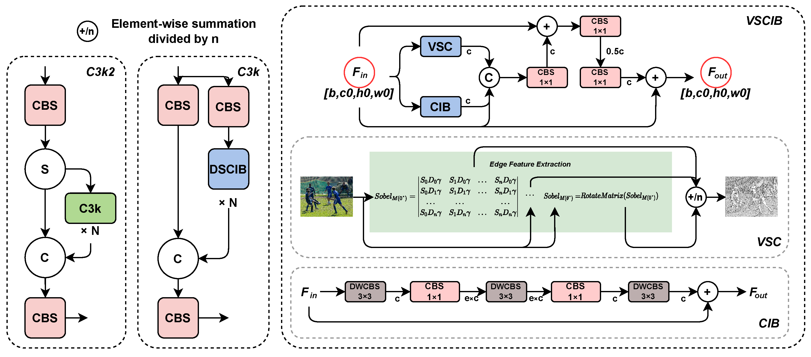
Figure 1. The network architecture: Variable Sobel Compact Inverted Block (VSCIB) for edge feature extraction; Spatial Pyramid Shared Convolution (SPSC) for multi-scale feature extraction; Efficient Down Convolution (EDC) for preserving key semantic information while reducing computational complexity. Note that CBS is a normal convolution module and executes in the order of Basic Convolution -> Batch Normalize(BN) -> Sigmoid linear unit(Silu) activation function.
Electronics 15 00449 g001
Figure 2. Architecture of the Variable Sobel Compact Inverted Block (VSCIB). The module combines Variable Sobel Convolution (VSC) for multi-directional edge extraction with a Compact Inverted Block (CIB) for efficient feature fusion. The Edge Feature Extraction block represents the process of extracting edge features.
Electronics 15 00449 g002
Figure 3. The two key matrices containing the optimal smoothing operator coefficient S m and the optimal difference operator coefficient D m . L represents the window size, and the coefficients correspond to their windows on the right.
Electronics 15 00449 g003
Figure 4. 3 × 3 Sobel Operator Templates for 8 Orientations.
Electronics 15 00449 g004
Figure 5. Architecture of the Efficient Downsampling Convolution (EDC) module and its integration in the detection head (EDC_Detect).
Electronics 15 00449 g005
Figure 6. Computational complexity reduction achieved by EDC and EDC_Detect modules across different network components.
Electronics 15 00449 g006
Figure 7. Spatial Pyramid Shared Convolution (SPSC). “Shared Conv” refers to Conv2d with shared convolution kernels and different dilation rates.
Electronics 15 00449 g007
Figure 8. Partial detection results from five representative object detection datasets: (a) RUOD (underwater scenes with marine life), (b) SVRDD (urban road environments with vehicles and pedestrians), (c) SHWD (construction sites focusing on helmet-wearing personnel), (d) PASCAL VOC (common indoor/outdoor objects such as bottles, cats, and chairs), and (e) MS COCO (complex, multi-object scenes spanning 80 categories). Bounding boxes are color-coded by class and annotated with confidence scores, illustrating the wide variation in domain, scale, occlusion, and scene complexity across benchmarks.
Electronics 15 00449 g008
Figure 9. The visualization results of these five datasets are used to showcase the characteristics of the datasets. Each image is divided into four parts, each providing different perspectives and information about the labels in the dataset. (a) RUOD; (b) SVRDD; (c) SHWD; (d) VOC; (e) COCO.
Electronics 15 00449 g009
Figure 10. We integrated the module into YOLOv11 and compared the detection performance of different modules on the VOC dataset.
Electronics 15 00449 g010
Figure 11. Comparison with Sobel, Canny, Laplacian, and Prewitt edge detection algorithms.
Electronics 15 00449 g011
Figure 12. Comparison of heat maps between EDC and Conv, DWConv, SCDond, Adown.
Electronics 15 00449 g012
Figure 13. Comparison between SPSC and SPPF in intermediate layers. (a) SPSC; (b) SPPF.
Electronics 15 00449 g013
Figure 14. Training progress of different ablation models in terms of mAP@0.5 (a) and mAP@0.5:0.95 (b) over epochs 150–380. (a) mAP@0.5 vs. epoch; (b) mAP@0.5:0.95 vs. epoch. Each curve corresponds to one model variant: (A) Baseline; (B) VSCIB; (C) VSCIB + EDC; (D) VSCIB + SPSC; (E) EDC + SPSC; (F) EDC; (G) SPSC; (H) Ours. The inset zooms into the final 100 epochs (300–380) to highlight convergence behavior.
Electronics 15 00449 g014
Figure 15. Normalized confusion matrices of the proposed model on five benchmark datasets: (a) RUOD, (b) SVRDD, (c) SHWD, (d) VOC, and (e) MS COCO. Each matrix visualizes the prediction distribution across classes, where rows represent ground truth labels and columns denote predicted labels. The color intensity reflects the normalized classification accuracy (ranging from 0 to 1), with darker shades indicating higher confidence in correct predictions.
Electronics 15 00449 g015
Figure 16. Visualize the object detection results of different object detection methods on five datasets. (a) Original, (b) YOLOv8n, (c) YOLOv10n, (d) YOLO11, (e) Ours.
Electronics 15 00449 g016
Table 1. Basic information and characteristics of the five datasets we used. Abbreviations denote meanings: Lab.: number of labeled objects. Cat.: number of categories. Bac.: image background. Specifically, S: specific location and G: general scene (covering complex objects and various environment challenges). HLE.: haze-like effects. CC.: color casts. CO.: complex objects. A checkmark (✔) indicates that this feature is present.
DatasetsImagesData SplitChallenges
Lab.Cat.Bac.TrainTestTolHLE.CC.CO.
RUOD [31]74,90310G9800420014,000
SVRDD [32]20,8047G600010007000
SHWD [33]120,5582S606415177581
VOC2007+2012 [34]40,05820G16,551495221,503
MS COCO2017 [35]846,68480G118,2875000123,287
Table 2. Comparison of different models. Bold numbers represent optimal values.
ModelsPrecision
(%)
Recall
(%)
mAP50
(%)
mAP50-95
(%)
Model Size
(MB)
Param
(M)
GFLOPs
C3k280.774.481.461.45.32.66.5
C2f80.474.081.160.66.02.96.7
C379.573.580.559.85.02.46.3
VSCIB (ours)80.974.882.062.75.52.66.6
Table 3. Comparative experiment of EDC on YOLO11. Bold numbers represent optimal values.
ModelsPrecision
(%)
Recall
(%)
mAP50
(%)
mAP50-95
(%)
Model Size
(MB)
Param
(M)
GFLOPs
Conv80.774.481.461.45.32.66.5
DWConv80.073.780.760.74.21.74.7
SCDown80.973.880.960.84.21.85.3
ADown79.473.179.457.74.42.04.5
EDC (ours)80.675.181.461.84.62.25.7
Table 4. Comparison of different spatial pyramid pooling modules. Bold numbers represent optimal values.
ModelsPrecision
(%)
Recall
(%)
mAP50
(%)
mAP50-95
(%)
Model Size
(MB)
Param
(M)
GFLOPs
SPPF80.774.481.461.45.32.66.5
SPP80.574.281.261.25.22.66.5
ASPP79.072.779.860.67.64.68.1
RFB82.073.682.062.15.92.86.6
SPSC (ours)80.675.482.562.65.82.76.5
Table 5. Comparison with state-of-the-art models on multiple datasets. Bold numbers represent optimal values.
ModelsRUODSVRDDSHWDPascal VOCMS COCOParam
(M)
GFLOPs
mAP50mAP50-95mAP50mAP50-95mAP50mAP50-95mAP50mAP50-95mAP50mAP50-95
Faster-RCNN [36]81.857.564.936.390.959.273.253.443.921.941.1463.3
RetinaNet [37]79.354.560.430.985.463.576.455.948.427.236.1739.7
FCOS79.554.060.232.285.863.978.458.756.137.431.8438.8
ATSS [38]80.356.963.634.989.457.879.858.655.638.331.8938.8
YOLOv5n81.464.861.735.891.357.879.358.152.437.42.57.1
YOLOv8n [39]84.767.463.536.892.260.180.460.152.137.33.28.7
YOLOv10n84.669.859.735.891.658.480.160.553.538.52.36.7
YOLOv11n84.967.963.137.592.259.581.461.454.939.52.66.5
Ours85.868.465.139.592.960.983.263.956.340.52.45.8
Table 6. Ablation study of different modules on VOC dataset. A checkmark (✔) indicates that the module exists. Bold numbers represent optimal values.
ModulesVSCIBEDCSPSCPrecision
(%)
Recall
(%)
mAP50
(%)
mAP50-95
(%)
Model Size
(MB)
Param
(M)
GFLOPsFPS
A (Baseline) 80.774.481.461.45.32.66.5115
B 80.974.882.062.75.52.66.6105
C 81.474.582.163.04.82.25.8124
D 81.574.882.563.25.82.86.5108
E 80.675.182.562.74.92.35.7128
F 82.273.081.461.84.62.25.7132
G 80.675.482.562.65.62.76.5112
H (Ours)80.376.683.263.95.22.45.8119
Disclaimer/Publisher’s Note: The statements, opinions and data contained in all publications are solely those of the individual author(s) and contributor(s) and not of MDPI and/or the editor(s). MDPI and/or the editor(s) disclaim responsibility for any injury to people or property resulting from any ideas, methods, instructions or products referred to in the content.