Reinforcement-Learning-Guided Two-Stage Multi-Energy Optimization for Carbon-Aware Charging Infrastructure

Abstract

Electric vehicle (EV) parking lots can create concentrated charging demand that couples operating cost, grid capacity use, and carbon emissions. This paper proposes a reinforcement-learning-guided two-stage multi-energy optimization framework for carbon-aware EV parking lot charging. The reinforcement learning (RL) layer uses a Deep Q-Network (DQN) to generate a data-driven charging reference from state-of-charge (SoC), time-to-departure, vehicle presence, electricity price, and grid-load information. This profile is transferred to a two-stage optimization model as a behavioral reference rather than being used as the final dispatch schedule. The first stage determines baseline operation and residual grid headroom, while the second stage schedules EV charging together with Power-to-Gas (P2G) and Carbon Capture and Storage (CCS) decisions under capacity, carbon-budget, and multi-energy constraints. A soft-tracking formulation links the learned profile with the optimized schedule and allows the tracking coefficient to shape different operating regimes. The results show that the proposed framework improves grid feasibility, reduces peak charging stress, and enhances carbon-aware operation. CCS mainly supports carbon-budget feasibility, whereas P2G provides additional value when renewable surplus is available.

1. Introduction

1.1. Motivation and Background

The electrification of transportation is increasing the pressure on distribution networks. Electric vehicles (EVs) reduce tailpipe emissions, but their charging demand creates new operational problems when many vehicles connect to the same local infrastructure within similar time windows [1,2]. This issue is especially visible in parking lots, campuses, workplaces, and public charging areas. In these locations, individual charging sessions can combine into a sharp aggregate peak and stress local feeders or transformer capacity [1,3].

Electric vehicle charging is different from many conventional loads. A vehicle often remains parked longer than the minimum time required to reach its desired state of charge (SoC). This creates operational flexibility. Charging can be delayed, accelerated, or redistributed over the parking duration if the required energy is delivered before departure [1,3]. At the same time, this flexibility is limited by user behavior. Arrival time, departure time, initial state of charge, and parking duration vary from one session to another. A charging strategy must therefore respond to both technical constraints and user-side variability.

Price-based scheduling can reduce operating cost, but it does not always protect the grid. If many vehicles react to the same low-price interval, charging demand may shift from one peak period to another [2,4,5]. A similar problem appears when charging is optimized only from the system perspective. Grid-friendly schedules may reduce peak loading, yet they can move away from the charging behavior observed in parking-lot data. For this reason, electric vehicle parking lot management should not be treated only as a cost-minimization task. It requires a coordinated formulation that links data-driven charging behavior with aggregate grid limits.

Carbon-aware operation adds another constraint to this problem. A schedule that is acceptable in terms of electricity cost may still be undesirable when carbon emissions are considered [6,7]. The problem becomes more complex when the parking lot is embedded in a multi-energy system. Power-to-Gas (P2G) can use surplus electrical energy through conversion, while Carbon Capture and Storage (CCS) can reduce net emissions associated with carbon-intensive operation [8,9,10]. These components provide additional flexibility, but their value depends on system conditions. Power-to-Gas is meaningful when surplus energy exists. Carbon Capture and Storage becomes important when the carbon budget is restrictive.

1.2. Related Work and Research Gap

Electric vehicle charging coordination has been studied through several modeling perspectives. Classical optimization methods are effective when the physical structure of the problem is known. They can represent charger limits, grid constraints, electricity prices, and departure requirements in a transparent way. Earlier studies formulated electric vehicle charging as an optimal control or scheduling problem under market prices and renewable availability [4,11]. Later works considered load limits, game-based coordination, and hosting capacity-oriented formulations to reduce the impact of charging on distribution systems [5,12,13]. These models are valuable because feasibility can be written directly into the formulation. Their main limitation is their dependence on assumed inputs. In real parking lot operation, arrival time, departure time, and initial state of charge vary across sessions.

Alternative model-based approaches have addressed uncertainty and sequential EV coordination through robust optimization and model predictive control. Distributionally robust energy management has been applied to multi-microgrid systems with grid-interactive EVs and temporally coupled user behavior [14]. Model predictive control studies have also examined EV integration, multi-source uncertainty, and charging-station operation in grid-connected microgrids [15,16,17]. These approaches provide model-based alternatives for predictive and constraint-aware scheduling.

Reinforcement learning (RL) has been used to address this behavioral variability, as reflected in recent reviews of EV charging and power-system applications [18,19]. The theoretical basis of reinforcement learning and Q-learning is well established [20,21], and Deep Q-Network (DQN) enabled value-based learning in high-dimensional decision problems [22]. In electric vehicle charging, model-free and deep reinforcement learning methods have been applied to real-time scheduling and coordinated charging control [23,24]. Broader safe reinforcement learning studies classify methods for constraint handling and risk reduction during policy learning [25,26]. EV-specific applications have subsequently incorporated operational constraints into deep reinforcement learning-based charging control [27,28]. These studies show that learning-based controllers can react to price, time, and system-state information without requiring a full deterministic model of user behavior. Still, strict aggregate feasibility remains difficult. A trained policy can generate a reasonable charging action for an individual session, but the resulting total profile may exceed the available system capacity.

Two-stage optimization provides a useful structure for separating baseline operation from flexible scheduling. In electric vehicle charging, this idea has been used to handle distribution-system constraints and uncertainty in charging demand [29]. It also fits naturally with mathematical programming tools such as General Algebraic Modeling System (GAMS), where energy balances and capacity limits can be expressed explicitly [30]. In this work, the two-stage structure is used to connect reinforcement learning with system-level scheduling. The first stage determines the baseline operation and the remaining headroom. The second stage uses that headroom to schedule electric vehicle charging and multi-energy operation. In this way, the learned charging profile is evaluated inside a feasible operating envelope rather than applied directly.

Carbon-aware scheduling has also become an important part of electric vehicle charging research. Cost minimization alone can move charging toward low-price hours, but this does not necessarily produce a low-emission schedule [6,7]. Carbon outcomes also depend on how electricity-related emissions are represented. Studies have examined marginal emission rates, the accuracy of simplified emission factors, and the implications of using average rather than marginal carbon-intensity signals in optimization [31,32,33]. Multi-objective electric vehicle charging models therefore consider carbon emissions together with charging cost and technical constraints [34]. Integrated energy system studies have also examined Power-to-Gas and Carbon Capture and Storage as flexibility options for low-carbon operation [8,9,10]. These technologies are not equivalent. Power-to-Gas is linked to surplus electrical energy, while Carbon Capture and Storage reduces net emissions subject to capture limits and operating cost. Their combined use is relevant for electric vehicle charging when the parking lot is modeled as part of a broader multi-energy system.

The reviewed literature leaves a specific gap at the interface between learned charging behavior and system-level feasibility. Existing optimization models can represent network, energy, and carbon constraints explicitly, but they usually rely on predefined charging demand or deterministic user assumptions. Learning-based methods can produce adaptive charging behavior from data, but their aggregate outputs still require validation against headroom and emission constraints. Moreover, multi-energy options such as P2G and CCS are rarely evaluated together with an RL-derived parking-lot charging profile. This paper addresses this gap by using the RL output as an input to a two-stage multi-energy optimization model rather than treating it as the final charging schedule. A comparative summary of the reviewed studies, highlighting their inclusion of key parameters such as EV charging, optimization, RL, carbon emissions, P2G, CCS, RL optimization coupling, uncertainty handling, and constraint hierarchy, is presented in

Table 1. Comparative taxonomy of recent studies on EV and multi-energy options.

Ref.	EV Charging	Optimization	RL	Carbon Emissions	P2G	CCS	RL–Optimization Coupling	Uncertainty	Constraint Hierarchy
[1]	✓	✓	×	×	×	×	×	M	M
[2]	✓	✓	×	×	×	×	×	M	M
[3]	✓	✓	×	×	×	×	×	D	H
[4]	✓	✓	×	×	×	×	×	D	H
[5]	✓	✓	×	×	×	×	×	A	H
[6]	✓	✓	×	✓	×	×	×	A	H
[7]	✓	✓	×	✓	×	×	×	D	H
[8]	×	×	×	✓	×	✓	×	—	—
[9]	×	✓	×	✓	✓	×	×	M	M
[10]	×	×	✓	✓	✓	✓	×	A	H
[11]	✓	✓	×	×	×	×	×	S	H
[12]	✓	✓	×	×	×	×	×	R	H
[13]	✓	✓	×	×	×	×	×	A	H
[14]	✓	✓	×	×	×	×	×	R	H
[15]	✓	✓	×	×	×	×	×	M	M
[16]	✓	✓	×	×	×	×	×	S + A	H
[17]	✓	✓	×	×	×	×	×	A	H
[18]	✓	×	✓	×	×	×	×	M	M
[19]	✓	×	✓	×	×	×	×	M	M
[20]	×	×	✓	×	×	×	×	—	—
[21]	×	×	✓	×	×	×	×	—	—
[22]	×	×	✓	×	×	×	×	—	—
[23]	✓	×	✓	×	×	×	×	A	P
[24]	✓	×	✓	×	×	×	×	A	P
[25]	×	×	✓	×	×	×	×	M	M
[26]	×	×	✓	×	×	×	×	M	M
[27]	✓	×	✓	×	×	×	×	A	H
[28]	✓	×	✓	×	×	×	×	A	H
[29]	✓	✓	×	×	×	×	×	S	H + P
[30]	×	✓	×	×	×	×	×	M	M
[31]	×	×	×	✓	×	×	×	—	—
[32]	×	×	×	✓	×	×	×	—	—
[33]	×	✓	×	✓	×	×	×	D	H
[34]	✓	✓	×	✓	×	×	×	D	H
[35]	×	✓	×	✓	✓	✓	×	D	H
[36]	×	✓	×	✓	✓	✓	×	D	H
This Study	✓	✓	✓	✓	✓	✓	✓	D*	H + P

✓: available; ×: not available; D: deterministic; S: stochastic; R: robust/DRO; A: adaptive/online; M: mixed/review; H: hard constraints; P: penalty/soft handling; H + P: hard and soft/penalty hierarchy; D*: deterministic formulation with forecast-error sensitivity.

.

1.3. Proposed Approach and Contributions

This paper develops a reinforcement-learning-guided two-stage multi-energy optimization framework for carbon-aware electric vehicle parking lot charging. The reinforcement learning layer uses a Deep Q-Network to generate a charging reference from real parking lot data. The first optimization stage determines baseline operation and calculates the remaining headroom for flexible scheduling. The second stage schedules electric vehicle charging within this headroom while coordinating Power-to-Gas and Carbon Capture and Storage decisions under carbon-budget and capacity constraints.

The connection between the learned profile and the optimized schedule is handled through a soft-tracking term. This allows the optimizer to follow the reinforcement learning reference when feasible and deviate from it when required by system constraints.

The main contributions of this paper are summarized as follows:

• A data-driven EV charging reference is generated from real parking lot data. A DQN agent uses SoC, time-to-departure, vehicle presence, electricity price, and grid-load information to learn session-level charging behavior over a 96-step daily horizon.
• A two-stage optimization structure is developed to convert the learned charging profile into a feasible system-level schedule. Stage 1 determines the baseline operation and residual grid headroom, while Stage 2 schedules EV charging under power-capacity, departure-energy, and carbon-budget constraints.
• A soft-tracking mechanism is introduced to couple RL and optimization without imposing the learned profile as a hard dispatch constraint. Positive and negative deviation variables, together with the tracking coefficient ${\lambda }_{RL}$, allow the optimizer to retain the RL charging pattern when feasible and modify it when system constraints become binding.
• The regime-dependent roles of CCS and P2G are evaluated within the same multi-energy framework. The analysis shows that CCS affects carbon-budget feasibility and the deliverable EV charging level, whereas P2G contributes to renewable-surplus utilization and operating-cost reduction in the surplus-enabled regime.

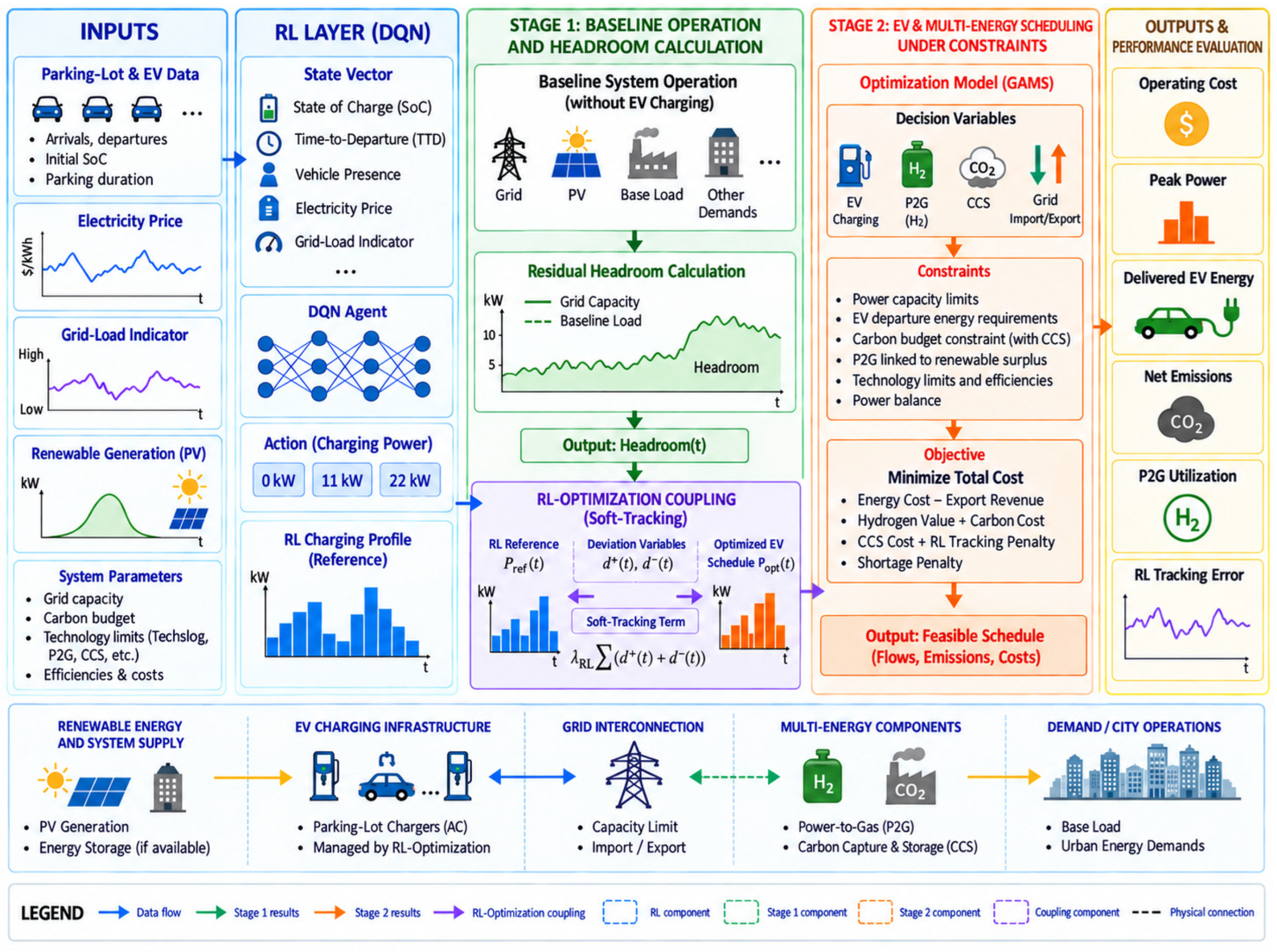
Figure 1 summarizes the complete workflow of the proposed framework, from input data and RL-based reference generation to two-stage optimization and performance evaluation. It also highlights the soft-tracking connection between the learned charging profile and the feasible optimized schedule. The remainder of this paper is organized as follows. Section 2 presents the parking lot data, the reinforcement-learning formulation, and the two-stage optimization model together with its soft-tracking coupling. Section 3 defines the experimental design, operating regimes, multi-energy scenarios, and performance metrics. Section 4 reports and discusses the numerical results. Section 5 concludes the paper.

2. Materials and Methods

2.1. Parking Lot Dataset

The study uses a real parking lot dataset that contains vehicle type information, arrival times, departure times, and initial state-of-charge values. The dataset is based on real-world data from a facility managed by İSPARK, which operates parking facilities throughout İstanbul/Türkiye. The raw data are organized as a two-dimensional matrix rather than a conventional vehicle-by-vehicle table. Each cell corresponds to a vehicle record at a specific parking location and scenario. The same cell coordinate is used across different sheets to reconstruct the full information of the vehicle.

The dataset contains separate sheets for internal combustion engine (ICE)/EV status, arrival time, departure time, and initial SoC. The EV status sheet identifies whether a given cell corresponds to an electric vehicle. The aligned cells in the remaining sheets provide the time-window and battery information. Invalid entries are removed before modeling. These include missing records, sentinel values such as −1000, and non-participating zero-valued records.

The first 100 of the 1000 scenarios were used. This positional subset closely matched the remaining 900 scenarios in initial SoC, arrival time, and parking duration (all standardized mean differences below 0.01), as well as in valid EV sessions per scenario (234.7 vs. 235.0). Scenarios 0–89 were used for training and 90–99 for held-out evaluation, corresponding to 21,118 and 2354 sessions, respectively, with no scenario-level overlap. The selected dataset includes 772 parking spots and 23,472 extracted EV sessions. The daily operation is represented by 96 time steps with a 15 min resolution. The assumed battery capacity is 75 kWh, the maximum charging power is 22 kW, and the charging target is 80% SoC.

2.2. Time Representation and Vehicle Presence

The arrival and departure values in the parking lot dataset are not stored as standard clock times. They are recorded as numerical values representing durations relative to the beginning of the operating day. Each value is first converted into minutes and then mapped to the common 15 min time grid. The main dataset and modeling parameters are summarized in

Table 2. Main Dataset and Modeling Parameters.

Parameter	Value
Total parking spots	772
Scenarios used	100 of 1000
Extracted EV sessions	23,472
Time resolution	15 min
Daily horizon	96 steps
Horizon length	24 h
Battery capacity	75 kWh
Maximum charger power	22 kW
SoC target	80%

. Let ${\Delta }_{\mathrm{a}\mathrm{r}\mathrm{r}}$ and ${\Delta }_{\mathrm{d}\mathrm{e}\mathrm{p}}$ denote the recorded arrival and departure values of a vehicle. The corresponding discrete time indices are calculated as:

$$t_{start}=⌊{\displaystyle \frac{round(60{\Delta }_{arr})}{\tau }}⌋,t_{end}=⌊{\displaystyle \frac{round(60{\Delta }_{dep})}{\tau }}⌋$$

(1)

where $\tau$ is the time-step duration. In this study, $\tau =15$ min and the daily horizon contain $T=96$ intervals. The calculated indices are clipped to remain within the feasible daily horizon.

The interval $\left[t_{\mathrm{s}\mathrm{t}\mathrm{a}\mathrm{r}\mathrm{t}},t_{\mathrm{e}\mathrm{n}\mathrm{d}}\right)$ defines the physical parking-presence window of the vehicle. Charging is allowed only inside this interval. The binary presence indicator is defined as

$$presence(t)=\left\{\begin{array}{cc}1,& t_{start}\le t<t_{end}\\ 0,& otherwise\end{array}\right.$$

(2)

The time-to-departure variable represents the remaining parking duration at each time step. It is measured in minutes and is used by the reinforcement learning agent as an urgency signal:

$$TTD(t)=max\left(0,(t_{end}-t)\tau \right)$$

(3)

The temporal preprocessing relations in (1)–(3) define the arrival index, departure index, vehicle-presence window, and time-to-departure information used throughout the framework. This representation is used consistently in the reinforcement learning environment, the exported RLData file, and the GAMS optimization model. It ensures that the learning output and the optimization input refer to the same vehicle-presence windows and the same 96-step daily horizon.

2.3. State-of-Charge and Charging Target

Each valid EV record includes an initial SoC value at arrival. The SoC is represented as a normalized value between 0 and 1. The nominal battery capacity is assumed to be 75 kWh, and the charging target is set to 80% of the battery capacity.

The SoC transition follows the charging energy added within a time step. If $\Delta E(t)$ denotes the requested charging energy at time step $t$, and $C_{\mathrm{b}\mathrm{a}\mathrm{t}}$ denotes the battery capacity, the next SoC is calculated in (4):

$$SoC(t+1)=SoC(t)+min[{\displaystyle \frac{\Delta E(t)}{C_{bat}}},max(0,{SoC}_{target}-SoC(t))]$$

(4)

where ${SoC}_{target}$ = 0.80. Charging is limited by the remaining target gap; an EV already at or above the target accepts no additional charging energy and retains its SoC.

At the aggregate level, the same energy representation is used to construct the exported RLData variables. The dataset records the aggregate EV stock before and after the charging action, arrival energy, departure energy requirement, and RL-achieved departure energy.

2.4. Electricity Price and Grid-Load Signals

The electricity buy price is aligned with the same 96-step horizon. The price signal contains four daily periods. The evening off-peak period covers 17:00–22:00 and ranges between 0.057 and 0.080 USD/kWh. The daytime mid-peak period covers 06:00–11:00 and ranges between 0.105 and 0.115 USD/kWh. The afternoon on-peak period covers 11:00–16:00 and reaches the highest range, between 0.120 and 0.161 USD/kWh. The night period covers 00:00–06:00 and ranges between 0.105 and 0.155 USD/kWh. A flat grid sell price of 0.030 USD/kWh is used. The electricity prices are based on Türkiye’s day-ahead electricity market operated by EPİAŞ: the day-ahead price profile of a representative (arbitrarily selected) market day is applied identically in all cases to ensure comparability [37].

A normalized grid-load indicator is also included in the reinforcement learning state. This signal allows the agent to distinguish low-stress and high-stress grid periods. The price and grid-load series are kept in the exported RLData file so that the learning-based profile can be interpreted under the same external conditions used in the optimization stage.

2.5. RL-to-Optimization Data Interface

The reinforcement learning output is exported as a tab-separated time-series dataset over the 96-step daily horizon. Each row corresponds to one time step. The index is written in a GAMS-compatible format from $t1$ to $t96$.

The main coupling variable is $P_{RL}(t)$. It represents the aggregate charging power produced by the trained reinforcement learning agent at time step t. In (5), for each evaluation session i, ${\Delta E}_i(t)$ denotes the realized charging energy within the vehicle-presence window, and the session-level contributions are aggregated as

$$P_{RL}(t)=\frac{{\sum }_{i\in I(t)}{\Delta E}_i(t)}{\Delta t},\hspace{1em}{E}_{RL}(t)=P_{RL}(t)\Delta t$$

(5)

Here, I(t) is the set of EV sessions present at time step t and Δt = 0.25 h; $E_{RL}(t)$ = $P_{RL}(t)$ Δt denotes the corresponding interval-energy signal. The exported file also includes aggregate charging power, grid-load indicator, buy price, normalized price, number of present EVs, arrival and departure counts, aggregate arrival energy, required departure energy, RL-achieved departure energy, and aggregate EV energy-stock variables.

In the optimization model, $P_{RL}(t)$ is used in the soft-tracking term introduced in Section 2.7.5. Therefore, the exported file provides the reference trajectory and the associated time-series inputs required for the GAMS model. The feasibility of the resulting charging schedule is determined later by the headroom, energy-balance, carbon-budget, and multi-energy constraints.

2.6. Reinforcement Learning Problem Formulation

The reinforcement learning layer is formulated as a Markov Decision Process (MDP). Each episode represents one EV charging session extracted from the preprocessed parking lot dataset. A session starts at the vehicle arrival time and ends at its departure time. During this interval, the agent observes the vehicle state and external signals, then selects one of the available charging actions [20].

At this stage, the learning problem is defined at the EV-session level. The DQN policy is trained to select charging actions during the vehicle presence window, using only the information available in its state vector. Aggregate grid, carbon, and multi-energy constraints are imposed neither during RL training nor during the rollout that generates the reference profile; they are introduced in the two-stage optimization model.

The MDP is represented by the tuple $\left(S,A,P,r,\gamma \right)$ where $S$ is the state space, $A$ is the action space, $P$ is the transition rule, $r$ is the reward function, and $\gamma$ is the discount factor. At each time step $t$, the agent observes $s_t$, selects an action $a_t$, receives the reward $r_t$, and moves to the next state according to the charging dynamics and the passage of time [21].

The state vector is designed to include the information needed for sequential EV charging decisions without making the learning problem unnecessarily large. At each time step, the agent observes battery status, departure urgency, time information, connection status, grid condition, and price information. The implemented state vector is

$$s_t=[SoC(t),TTD(t),t,presence(t),g(t),{\pi }_{norm}(t)]$$

(6)

In (6), $SoC(t)$ is the normalized state of charge, $TTD(t)$ is the remaining time before departure, $t$ is the discrete time index, $presence(t)$ indicates whether the EV is physically connected, $g(t)$ is the normalized grid-load indicator, and ${\pi }_{norm}$(t) is the normalized electricity price signal.

The state input remains six-dimensional; however, because each training episode spans only the vehicle-presence interval, the presence flag is constant during the current session-based training. The time-to-departure variable gives urgency to the policy. When departure is far away, the agent can postpone charging during high-price or high-load periods. When the remaining time becomes short, the same policy is pushed toward completion-oriented charging.

The charging controller uses a discrete action space with three charging levels. This is suitable for DQN because the method estimates one Q-value for each available action. The action set is $A=\{\mathrm{0,1},2\}$ in (7) and the mapping from action index to charging power is:

$$P_{ch}(a_t)=\left\{\begin{array}{cc}0,& a_t=0\\ 11,& a_t=1\\ 22,& a_t=2\end{array}\right.$$

(7)

The idle action represents no charging. The moderate charging action corresponds to 11 kW, and the fast-charging action corresponds to 22 kW. This three-level structure keeps the action space interpretable and reflects the operational charging levels. For a 15 min time step, the charging energy requested by the selected charging action is calculated in (8) as:

$$\Delta E(t)=P_{ch}(t){\displaystyle \frac{\tau }{60}}$$

(8)

where $P_{ch}(t)$ is in kW, $\tau$ is in minutes, and $\Delta E(t)$ is in kWh. Since $\tau =15$, the selected power is converted into energy over a quarter-hour interval. The accepted charging energy and SoC transition follow (4).

The reward function is designed to guide the agent toward practical charging behavior. It encourages energy delivery within the parking window and discourages charging during expensive or high-load intervals. A departure penalty is applied when the vehicle leaves without reaching the target SoC. Here, ΔE(t) denotes the charging energy actually accepted under (4). In (9), when the agent charges, it receives a positive energy reward:

$$r_t^{energy}=\Delta E(t)$$

(9)

Grid-load and price penalties are applied in (10):

$$r_t^{grid}=-\alpha g\left(t\right)\Delta E\left(t\right),r_t^{price}=-\beta {\pi }_{norm}(t)\Delta E(t)$$

(10)

where $\alpha$ and $\beta$ control the relative weights of grid-load awareness and price awareness.

The departure penalty is

$$r_t^{dep}=\left\{\begin{array}{cc}-\kappa {\displaystyle \frac{{SoC}_{target}-SoC(t+1)}{{SoC}_{target}}},& TTD(t+1)=0\mathrm{a}\mathrm{n}\mathrm{d}SoC(t+1)<So{C}_{target}\\ 0,& \mathrm{o}\mathrm{t}\mathrm{h}\mathrm{e}\mathrm{r}\mathrm{w}\mathrm{i}\mathrm{s}\mathrm{e}\end{array}\right.$$

(11)

This term in (11) penalizes the agent if the session ends below the target SoC. The reward components also include the numerical weights used in training: $\alpha =2.0$, $\beta =1.5$, and κ = 50.0.

The total reward combines these components in (12):

$$r_t=r_t^{energy}+r_t^{grid}+r_t^{price}+r_t^{dep}$$

(12)

The DQN agent approximates the action-value function $Q(s,a)$. The input layer receives the six-dimensional state vector, and the output layer produces one Q-value for each action. This approach uses two fully connected hidden layers with 64 neurons and ReLU activation. The output layer has three linear neurons corresponding to the three charging actions.

Training uses experience replay and a target network. These mechanisms reduce instability in value-based learning. The replay buffer stores past transitions, and mini-batches are sampled during training. The target network is updated periodically to stabilize the temporal-difference target [22]. The main DQN configuration is summarized in

Table 3. DQN Agent Configuration.

Parameter	Value
State dimension	6
Action space	3 actions
Network architecture	2 × 64 dense layers with ReLU
Learning rate	0.001
Discount factor	0.95
Replay buffer size	10,000
Batch size	64
Initial exploration rate	1.0
Minimum exploration rate	0.01
Exploration decay	0.998 per replay update (every 4 environment steps, after buffer warm-up)
Target update frequency	10 episodes
Training episodes	1500
Training frequency	Every 4 steps

.

The training process uses an ϵ-greedy strategy. Early episodes contain more exploration, while later episodes increasingly exploit the learned Q-values. The practical training objective is not to prove global optimality of the RL controller. The goal is to obtain a stable and interpretable charging profile that reacts to SoC, time-to-departure, price, and grid-load conditions.

Using the split defined in Section 2.1, no separate validation subset was used. Representative results use seed 42, while seeds 43 and 44 repeat the same DQN configuration for multi-seed evaluation. Each 1500-episode run samples training sessions with replacement; generalization is assessed on the held-out fleet scenarios.

After training, the learned policy is evaluated using the session-to-aggregate procedure in Section 2.5. This profile is exported as RLData and transferred to the optimization model.

2.7. Two-Stage Multi-Energy Optimization and RL–GAMS Coupling

The optimization layer is implemented as a two-stage linear programming model. The first stage determines the baseline system operation without directly scheduling EV charging. Its main output is the remaining grid headroom available for flexible EV demand. The second stage uses this headroom to schedule EV charging together with the multi-energy components [29]. The RL profile provides a soft reference rather than a hard schedule.

The optimization model is formulated as a deterministic full-horizon day-ahead planning problem. The nominal results therefore assume that the required EV-availability, baseline-load, and renewable-generation information is available over the 96-step horizon; the sensitivity of this assumption is examined in Section 4.9.

The time horizon is represented by the set $t\in T$, where $T=96$ and each time step corresponds to $\Delta t=0.25$ h. The same time index is used in RLData and in the GAMS model [30]. This keeps the learned profile, baseline load, renewable generation, EV availability, and electricity price aligned over the full daily horizon.

2.7.1. Stage 1: Baseline System Optimization and Headroom Calculation

Stage 1 represents the non-EV baseline system. It includes baseline demand, grid import, renewable generation, emissions, and carbon capture variables. The purpose of this stage is to determine how much of the grid connection capacity is already occupied by the non-EV system operation. The remaining part of the connection capacity is then passed to Stage 2 as the EV charging headroom.

The Stage 1 objective minimizes the operating cost of the baseline system and the carbon cost associated with net emissions:

$$z_1=\sum _{t\in T}\left[{\pi }_{buy}(t)P_{base}(t)\Delta t+c_{CO2}{E}_{net,1}(t)\right]$$

(13)

Here, ${\pi }_{\mathrm{b}\mathrm{u}\mathrm{y}}(t)$ is the grid electricity buy price, $P_{\mathrm{b}\mathrm{a}\mathrm{s}\mathrm{e}}(t)$ is the grid power used by the baseline system, $c_{\mathrm{C}\mathrm{O}2}$ is the carbon cost coefficient, and $E_{\mathrm{n}\mathrm{e}\mathrm{t},1}(t)$ is the net emission after carbon capture.

The baseline power balance is written as

$$P_{base}(t)+P_{RES}(t)\ge D_{base}(t)$$

(14)

where $P_{\mathrm{R}\mathrm{E}\mathrm{S}}(t)$ is renewable generation, $D_{\mathrm{b}\mathrm{a}\mathrm{s}\mathrm{e}}(t)$ is the non-EV baseline demand. Stage-1 P2G is zero in all reported cases because the implemented baseline model contains no P2G decision variable. The inequality form allows renewable production above the baseline demand to appear as available surplus instead of forcing artificial grid consumption.

The baseline grid import is limited by the grid connection capacity:

$$P_{base}(t)\le P_{cap}$$

(15)

Gross and net emissions in Stage 1 are calculated as

$$E_{gross,1}\left(t\right)=e{f}_{grid}{P}_{base}\left(t\right)\Delta t,E_{net,1}(t)=E_{gross,1}(t)-E_{CCS,1}(t)$$

(16)

The carbon capture amount is bounded by the capture capacity and by the available gross emissions:

$$E_{CCS,1}\left(t\right)\le E_{CCS}^{max},E_{CCS,1}(t)\le E_{gross,1}(t)$$

(17)

After solving Stage 1, the remaining grid headroom is calculated as

$$P_{max}(t)=P_{cap}-P_{base}^{\ast }(t)$$

(18)

where $P_{\mathrm{b}\mathrm{a}\mathrm{s}\mathrm{e}}^{\ast }(t)$ is the optimized baseline grid import. This headroom is one of the most important links between the two stages. It prevents the EV charging schedule in Stage 2 from exceeding the residual grid capacity.

The renewable surplus passed from Stage 1 to Stage 2 is calculated as

$$P_{sur}(t)=max[0,P_{RES}(t)-D_{base}(t)]$$

(19)

This variable represents the renewable power that remains available after the baseline demand is served. It is later used in Stage 2 for surplus-enabled P2G operation. Together, (13)–(19) define the Stage-1 objective, baseline operating constraints, residual grid headroom, and renewable-surplus calculation.

2.7.2. Stage 2: EV and Multi-Energy Scheduling

Stage 2 schedules EV charging under the headroom obtained from Stage 1. It also coordinates grid import, renewable surplus utilization, P2G conversion, CCS operation, grid export, and possible unmet departure energy. The optimized EV charging profile is therefore constrained not only by charger availability, but also by grid capacity and carbon-budget limits.

The Stage 2 objective is:

$$\begin{gathered} z_2=\sum _{t\in T}\left[{\pi }_{buy}\left(t\right)P_{buy,2}\left(t\right)\Delta t-{\pi }_{sell}\left(t\right)P_{sell,2}\left(t\right)\Delta t-v_{H2}{\eta }_{P2G}{P}_{P2G,2}\left(t\right)\Delta t+c_{CO2}{E}_{net,2}(t)+c_{CCS}{E}_{CCS,2}\left(t\right)\right]+ \\ {\lambda }_{RL}\sum _{t\in T}\left[d^{+}(t)+d^{-}(t)\right]+c_{short}\sum _{t\in T}{E}_{short}(t) \end{gathered}$$

(20)

The first part of the objective represents the physical operating cost. It is defined in Section 3.5. The second part penalizes deviation from the RL reference profile. The last part penalizes unmet departure energy. The Stage 2 power balance is:

$$P_{buy,2}(t)+P_{V2G}(t)+P_{sur}(t)=P_{EV}(t)+P_{P2G,2}(t)+P_{sell,2}(t)+P_{curt,2}(t)$$

(21)

Here, $P_{\mathrm{b}\mathrm{u}\mathrm{y},2}(t)$ is grid import, $P_{\mathrm{V}2\mathrm{G}}(t)$ is vehicle-to-grid (V2G) discharge power, $P_{\mathrm{s}\mathrm{u}\mathrm{r}}(t)$ is renewable surplus from Stage 1, $P_{\mathrm{E}\mathrm{V}}(t)$ is aggregate EV charging power, $P_{\mathrm{P}2\mathrm{G},2}(t)$ is P2G power, $P_{\mathrm{s}\mathrm{e}\mathrm{l}\mathrm{l},2}(t)$ is grid export, and $P_{\mathrm{c}\mathrm{u}\mathrm{r}\mathrm{t},2}(t)$ is unused renewable surplus. In the reported implementation, V2G is structurally disabled by setting its maximum power to zero.

The Stage 2 grid import cannot exceed the headroom from Stage 1:

$$P_{buy,2}(t)\le P_{max}(t)$$

(22)

Aggregate EV charging is also limited by the number of connected EVs:

$$P_{EV}(t)\le P_{charger}^{max}{N}_{EV}(t)$$

(23)

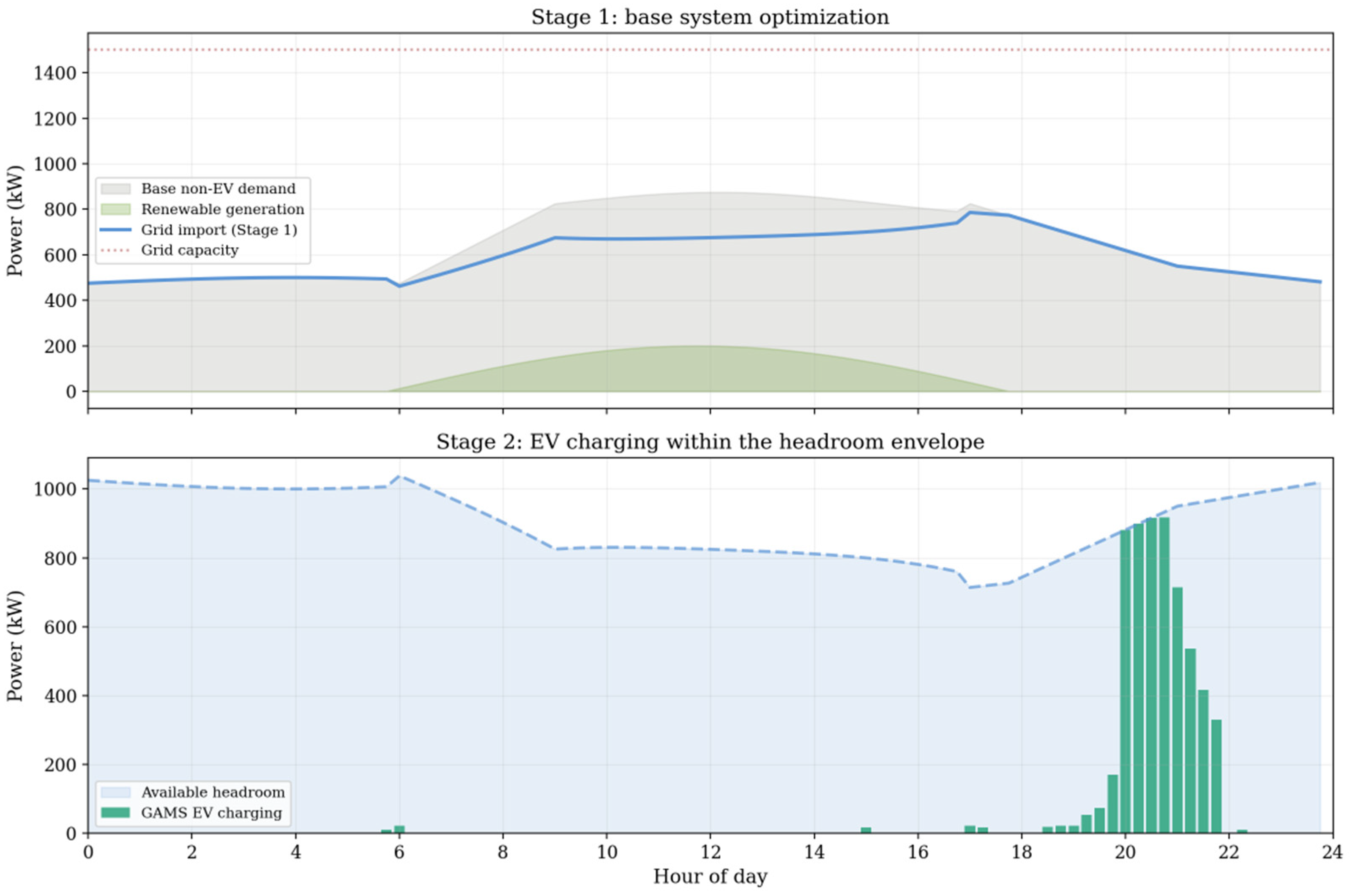
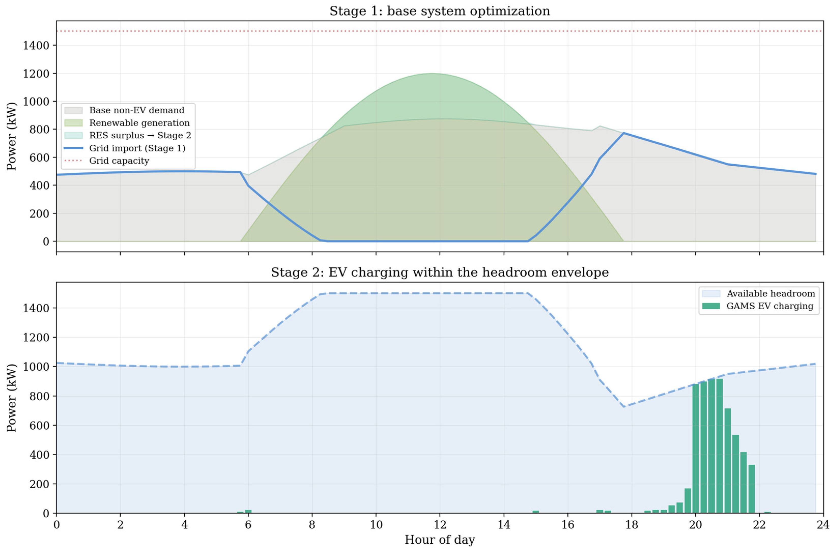
This constraint prevents the optimizer from assigning more charging power than the connected EV population can physically receive. The Stage 2 objective and its main power and capacity constraints are given in (20)–(23). Figure 2 illustrates the two-stage RL–GAMS coupling structure used in the load-dominant regime.

2.7.3. Carbon Budget and CCS Constraints

Carbon emissions in Stage 2 are calculated only from grid import. Renewable surplus does not create grid-related emissions in the model. For each optimization run, grid-related emissions are calculated using a constant representative emission factor, ${ef}_{grid}$; temporal variations in grid carbon intensity are not modeled within the 24 h horizon. Accordingly, ${ef}_{grid}$ should be interpreted as a constant representative average emission factor for the modeled case rather than a time-resolved marginal carbon-intensity signal [38]. Gross emissions are therefore defined as

$$E_{gross,2}(t)=e{f}_{grid}{P}_{buy,2}(t)\Delta t$$

(24)

Net emissions are calculated after CCS operation:

$$E_{net,2}(t)=E_{gross,2}(t)-E_{CCS,2}(t)$$

(25)

The total Stage 2 net emission is

$$E_{total,2}=\sum _{t\in T}{E}_{net,2}(t)$$

(26)

The carbon-budget constraint is then written as

$$E_{total,2}\le E_{budget}$$

(27)

CCS operation is limited by the capture capacity and by the gross emissions available at each time step:

$$E_{CCS,2}(t)\le E_{CCS}^{max}$$

(28)

$$E_{CCS,2}(t)\le E_{gross,2}(t)$$

(29)

These constraints ensure that CCS cannot capture more emissions than the system produces [35]. CCS is represented as a bounded CO₂-capture decision with an operating-cost term; detailed capture-energy requirements, transport, storage dynamics, and life-cycle emissions are outside the present model boundary. Relations (24)–(29) define gross and net emissions, the total carbon budget, and the CCS operating limits. In the optimization model, CCS becomes important when the carbon budget is restrictive and additional EV charging would otherwise violate the emission limit.

2.7.4. P2G Modeling Under Renewable Surplus

P2G is modeled as a surplus-linked conversion option [36]. It can absorb renewable surplus and generate hydrogen value in the objective function. The conversion power is limited by the P2G unit capacity:

The hydrogen-energy output credited in the objective is obtained from the P2G electrical input using ${\eta }_{P2G}$ = 0.65; $v_{H2}$ is therefore expressed per kWh of hydrogen-energy output.

$$P_{P2G,2}(t)\le P_{P2G}^{max}$$

(30)

The key physical constraint is that P2G cannot consume more power than the renewable surplus available at the same time step:

$$P_{P2G,2}(t)\le P_{sur}(t)$$

(31)

This constraint prevents grid-powered P2G operation. When renewable surplus is zero, P2G is forced to zero as defined in (30) and (31). In the load-dominant regime, renewable generation peaks at 200 kW while $D_{base}$(t) ≥ 400 kW, so Stage 2 P2G is structurally zero. As a result, P2G cannot be used as a grid-arbitrage mechanism. Its role is limited to utilizing renewable surplus that would otherwise be exported or curtailed.

This distinction is important for interpreting the results. P2G does not generally increase EV charging feasibility under a tight carbon budget. Its main contribution appears in the surplus-enabled regime, where renewable excess is available. CCS, on the other hand, directly reduces net emissions within the model and can therefore support EV charging under the carbon-budget constraint.

Figure 2 and Figure 3 illustrate the same two-stage optimization logic under the load-dominant and surplus-enabled regimes, respectively. Their comparison highlights how renewable surplus changes flexibility allocation and activates P2G without altering the core scheduling structure.

2.7.5. RL Soft-Tracking Formulation

The coupling between the RL output and the Stage 2 decision variable is modeled through positive and negative deviation variables. This formulation in (32) avoids an equality constraint between $P_{EV}$ (t) and $P_{RL}$ (t) while still assigning a cost to deviations from the learned profile. The tracking relation is written as:

$$P_{EV}\left(t\right)-P_{RL}\left(t\right)=d^{+}\left(t\right)-d^{-}\left(t\right),\hspace{1em}{d}^{+}\left(t\right)\ge 0,\hspace{1em}{d}^{-}(t)\ge 0$$

(32)

Here, $P_{RL}$(t) is the aggregate charging power produced by the RL policy, and d + (t) and d − (t) are positive and negative deviation variables. The sum of these deviations is penalized in the objective by ${\lambda }_{\mathrm{R}\mathrm{L}}$. Because the objective sums absolute power deviations over the time intervals, ${\lambda }_{\mathrm{R}\mathrm{L}}$ is expressed in USD/kW; multiplying the same sum by Δt gives the energy-based tracking measure in Section 3.5.

A low value of ${\lambda }_{\mathrm{R}\mathrm{L}}$ makes the optimizer more willing to deviate from the learned profile. A high value of ${\lambda }_{\mathrm{R}\mathrm{L}}$ places greater weight on following the RL reference. This parameter therefore controls the balance between behavioral tracking and system-level optimization.

2.7.6. Aggregate EV Energy Balance and Departure Service

The EV energy state is modeled at the aggregate level. This is consistent with the RLData interface, where individual vehicle actions are transformed into a time-indexed aggregate charging profile. The aggregate EV stock-flow dynamics, departure-service requirements, and global energy-consistency condition are represented in (33)–(37).

At the first time step, the aggregate EV energy is initialized as

$$E_{EV}(1)=E_{EV}^{init}+\Delta t{P}_{EV}(1)-\Delta t{P}_{V2G}(1)$$

(33)

For the remaining time steps, the aggregate EV energy evolves as

$$E_{EV}(t)=\left(1-{\alpha }_{dep}(t)\right)E_{EV}(t-1)+E_{arr}(t)+\Delta t{P}_{EV}(t)-\Delta t{P}_{V2G}(t)$$

(34)

where ${\alpha }_{\mathrm{d}\mathrm{e}\mathrm{p}}\left(t\right)$ represents the fraction of connected EV energy leaving the parking lot at time step $t$, and $E_{\mathrm{a}\mathrm{r}\mathrm{r}}(t)$ is the energy brought by newly arriving EVs. The aggregate EV energy is limited by the maximum energy capacity of the connected EV population:

$$E_{EV}(t)\le E_{EV}^{max}(t)$$

(35)

Departure service is represented through served and unmet departure energy:

$$E_{dep}^{served}\left(t\right)+E_{short}\left(t\right)=E_{dep}^{req}\left(t\right),\hspace{1em}{E}_{EV}(t)\ge E_{dep}^{served}(t)$$

(36)

The unmet term $E_{\mathrm{s}\mathrm{h}\mathrm{o}\mathrm{r}\mathrm{t}}(t)$ is penalized in the objective. This prevents the optimizer from satisfying grid or carbon constraints by simply ignoring the departure energy requirement. The global EV energy consistency condition is

$$E_{V2G}^{total}+E_{dep}^{served,total}\le E_{EV}^{init}+E_{arr}^{total}+E_{EV}^{charge,total}$$

(37)

This constraint ensures that the total discharged and served departure energy cannot exceed the initial energy, arrival energy, and charged energy available in the aggregate EV stock. The main optimization parameters and input assumptions are consolidated in

Table 4. Consolidated optimization parameters and input assumptions.

Parameter/İnput	Value/Regme	Meaning	Source/Basis
$P_{cap}$	1500 kW	Grid connection capacity	Assumption
$E_{budget}$	0.50 tCO2	Daily Stage-2 carbon budget	Assumption; sensitivity in Section 4.6
${ef}_{grid}$	0.00047 tCO2/kWh	Constant representative grid emission factor	Republic of Türkiye Ministry of Energy and Natural Resources [38]
$c_{CO2}$	50 USD/tCO2	Carbon cost coefficient	Assumption
$E_{CCS,max}$	0.050 tCO2/step	Maximum capture per interval	Assumption
$c_{CCS}$	20 USD/tCO2	Capture operating cost	Assumption
$P_{P2G,max}$	200 kW	P2G electrical input capacity	Assumption
${\eta }_{P2G}$	0.65	Electricity-to-hydrogen energy conversion efficiency	Literature-informed [39]
$v_{H2}$	0.08 USD/kWhH2	Hydrogen-energy output value	Assumption
${\pi }_{sell}$	0.030 USD/kWh	Grid export price	Input data: Grid Price.xlsx
$C_{short}$	50 USD/kWh	Unserved-energy penalty	Assumption
$P_{V2G,max}$	0 kW	V2G disabled	Model setting
Δt	0.25 h	Interval duration	Model time resolution
${\lambda }_{RL}$	1 USD/kW	Reference power-tracking weight	Selected value; sensitivity in Section 4.4
$P_{RES,peak}$	200/1200 kW	Load-dominant/surplus-enabled renewable peak	Assumption
$P_{RES}$(t)	Half-sine; 24 < t < 72	PRES,peak sin[π(t − 24)/48]; zero otherwise	Assumption
$D_{Base}$ (t)	400 + 500G(t) kW	Non-EV baseline demand	Assumption
${\pi }_{buy}$(t)	0.057–0.161 USD/kWh	Time-varying grid purchase price	Input data: Grid Price.xlsx; Section 2.4

.

Basis distinguishes source/data-based inputs, literature-informed assumptions, and case-study model assumptions.

3. Experimental Design and Evaluation Methodology

The numerical study is designed to evaluate how the learned RL charging profile behaves when it is placed under system-level grid and carbon constraints. The experiment uses the same 96-step daily horizon adopted in the data preprocessing and RL training stages. Each time step corresponds to 15 min, so all charging, grid, emission, and multi-energy variables are evaluated over a 24 h operating period.

The experimental workflow has three main steps. First, the trained DQN policy is rolled out using the parking lot data and generates the RL charging profile. Second, the Stage 1 optimization model calculates the baseline system operation and the residual grid headroom. Third, the Stage 2 model schedules EV charging and multi-energy operation by using the RL profile as a soft reference.

All compared cases use the same time horizon, price series, vehicle availability data, and emission parameters. Differences between the cases therefore come from the scheduling structure and the active multi-energy components rather than from changes in the input data.

End-to-end robustness was evaluated across held-out fleet scenarios 90–99 and DQN seeds 42–44, yielding 30 seed–scenario combinations per operating regime. These are fleet scenarios rather than calendar days; electricity-price and base-load profiles remain fixed. Scenario SD and seed SD denote the sample SDs of the ten scenario means and three seed means, respectively.

3.1. Compared Scheduling Cases

Three scheduling cases are considered in the evaluation. These cases are summarized in

Table 5. Compared scheduling cases.

Case	Description	Main Role
RL-only	Charging profile generated directly by the trained DQN policy	Behavioral reference
Optimization-only	EV schedule obtained mainly from the mathematical optimization model	Constraint-driven benchmark
RL-guided optimization	GAMS schedule with soft tracking of the RL profile	Proposed hybrid case

. The first case is the RL-only reference. In this case, the charging profile is obtained directly from the trained DQN policy. It represents learned charging behavior, but it is not corrected by the optimization model.

The second case is the optimization-only schedule. In this case, the optimizer schedules EV charging without being forced to follow the RL charging shape. This case is useful for identifying the cost- or constraint-driven behavior of the mathematical model when behavioral tracking is weak or absent.

The third case is the RL-guided optimized schedule. In this case, the RL profile is included through the soft-tracking term. The optimizer follows the learned reference when possible, but it is allowed to deviate from it when grid headroom, carbon budget, or multi-energy constraints require a different schedule. This is the main hybrid case of the study.

3.2. Operating Regimes

Two operating regimes are evaluated. The first regime is the load-dominant regime. In this regime, renewable surplus is not available for P2G operation. Therefore, the P2G component remains inactive. This regime is useful for observing the role of CCS and grid headroom when EV charging must mainly be supplied through the grid.

The second regime is the surplus-enabled regime. In this regime, renewable production can exceed the non-EV baseline demand at some time steps. The remaining surplus can then be used by the P2G unit. This regime is needed to evaluate whether P2G provides a cost or utilization benefit when surplus energy exists.

The two regimes are not used to change the RL policy. The learned RL reference remains the same. What changes is the energy-system condition under which the optimization model tries to schedule EV charging. This separation, shown in

Table 6. Operating regimes.

Regime	Renewable Surplus	P2G Availability	Main Interpretation
Load-dominant	No effective surplus	Inactive	Grid and CCS constrained charging
Surplus-enabled	Available at selected intervals	Active within surplus limit	Surplus utilization through P2G

, makes it possible to identify whether the improvement comes from the learned charging behavior, the grid-capacity correction, the carbon constraint, or the multi-energy components.

3.3. Multi-Energy Activation Configurations

Four multi-energy configurations are used to isolate the individual and combined effects of P2G and CCS. The electricity-only case is used as the reference. P2G-only, CCS-only, and combined P2G–CCS cases are then compared against this reference. The configurations are defined in

Table 7. Multi-energy activation configurations.

Scenario	P2G	CCS	Description
M0	Off	Off	Electricity-only operation
M1	On	Off	Electricity + P2G
M2	Off	On	Electricity + CCS
M3	On	On	Electricity + P2G + CCS

.

3.4. RL-Tracking Weight Scenarios

The hybrid model includes the RL-tracking coefficient ${\lambda }_{RL}$. This parameter controls how strongly the Stage 2 optimizer follows the RL reference. A small value allows larger deviations from the RL profile, while a larger value gives greater priority to behavioral tracking.

The tracking behavior is evaluated by varying ${\lambda }_{RL}$ across a selected range. This creates a trade-off between physical optimization and RL-following behavior. When ${\lambda }_{RL}$ is very small, the optimizer is dominated by physical cost and system constraints. When ${\lambda }_{RL}$ is sufficiently large, the optimized schedule moves closer to the RL profile as long as the system constraints allow it.

This analysis is necessary because a hybrid RL–optimization model should not be judged at only one tracking weight. A single value of ${\lambda }_{RL}$ may hide whether the model is actually following the RL profile or simply ignoring it. The weight sweep therefore shows the operating region where the model changes from optimization-dominant behavior to RL-guided behavior.

3.5. Performance Metrics

The performance evaluation uses both physical and behavioral metrics summarized below. Physical metrics are needed to evaluate system operation. Behavioral metrics are needed to evaluate how closely the optimized schedule follows the RL reference.

The main energy metric is the total EV charging energy:

$$E_{EV}^{charge}=\sum _{t\in T}{P}_{EV}(t)\Delta t$$

(38)

The peak grid import is used to evaluate the maximum stress imposed on the grid connection:

$$P_{grid}^{peak}=\underset{t\in T}{max}{P}_{grid}(t)$$

(39)

The total net emission is calculated from the sum of time-step net emissions:

$$E_{net}^{total}=\sum _{t\in T}{E}_{net}(t)$$

(40)

Carbon intensity is used to compare the emissions associated with delivered EV charging energy:

$$C{I}_{EV}={\displaystyle \frac{E_{net}^{total}}{E_{EV}^{charge}}}$$

(41)

The RL-tracking error is calculated as the time-integrated absolute deviation between the optimized EV charging power and the RL reference, in kWh:

$${D_{RL}}^E=\sum _{t\in T}\mid P_{EV}(t)-P_{RL}(t)\mid \Delta t$$

(42)

Headroom-violation energy is defined as $E_{viol}={\sum }_{t}max[0,P_{EV}(t)-P_{max}(t)]\Delta t$ in kWh for each compared schedule. Both energy-based deviation metrics use Δt = 0.25 h.

The departure-service metric is represented by unmet departure energy. A lower value indicates that the optimized schedule satisfies more of the required departure energy:

$$E_{short}^{total}=\sum _{t\in T}{E}_{short}(t)$$

(43)

Together, Equations (38)–(43) define the energy, peak-power, emission, carbon-intensity, RL-tracking, and departure-service metrics used in the evaluation.

Physical operating cost equals grid purchase cost minus export revenue and hydrogen value, plus carbon-emission cost and CCS operating cost. It excludes RL-tracking and departure-shortage/service penalties.

4. Results and Discussion

This section evaluates the proposed RL-guided two-stage optimization framework from three perspectives. First, the raw RL profile is examined as a behavioral charging reference. Second, the ability of the GAMS model to restore feasibility under grid-headroom and carbon constraints is analyzed. Third, the roles of P2G and CCS are evaluated under load-dominant and surplus-enabled operating regimes.

4.1. RL-Only Charging Behavior

The RL-only profile represents the charging behavior generated by the trained DQN policy before system-level correction. This profile is useful because it shows how the learning agent reacts to parking duration, SoC, price, and grid-load signals. It also provides the reference that is later used in the GAMS optimization layer.

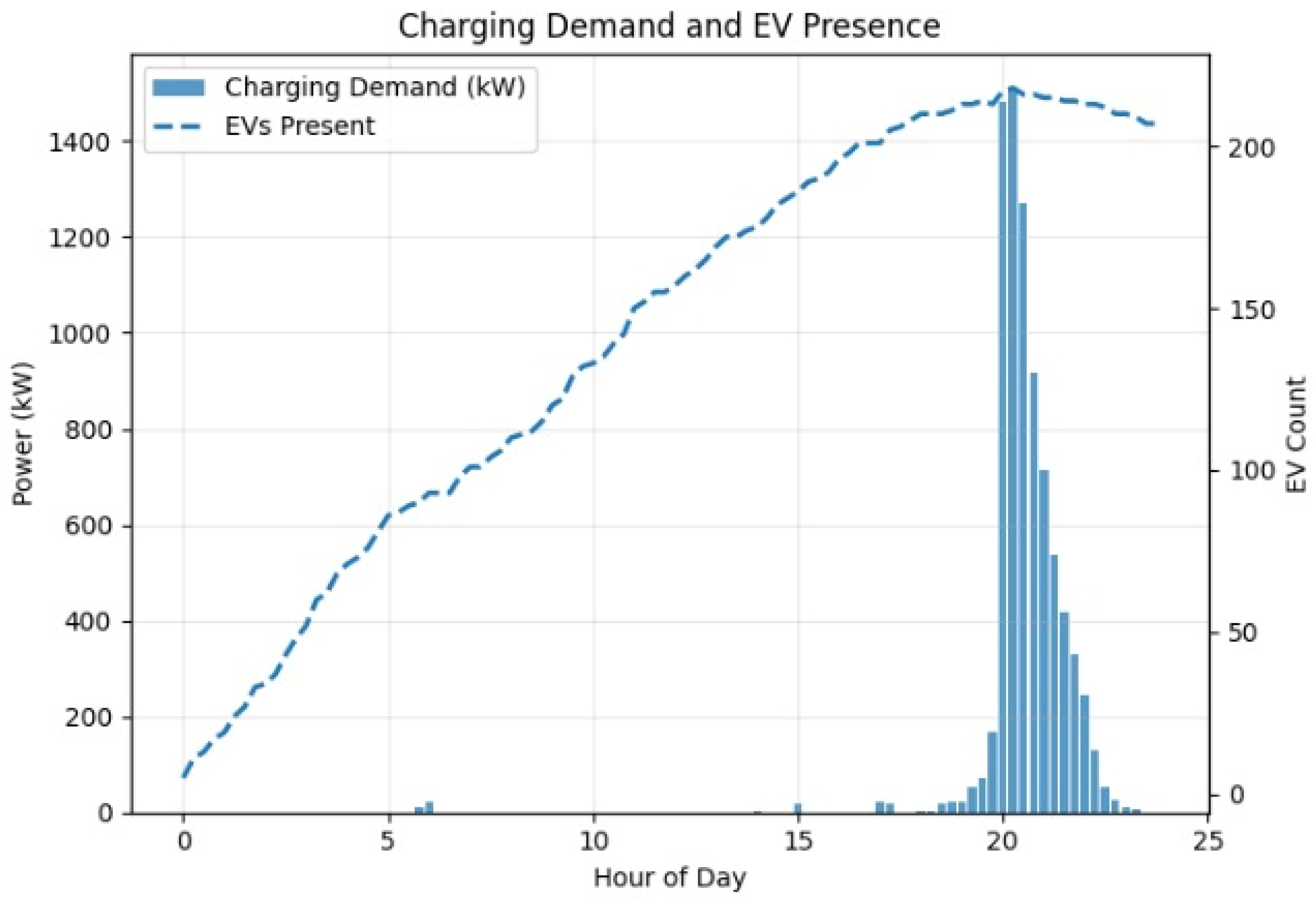
The aggregate RL profile shows a visible concentration of charging demand during low-price periods. This behavior is consistent with the price signal included in the state vector and the reward structure used during training. However, this profile is obtained before applying the Stage 1 headroom constraint. Its feasibility must be evaluated at the system level rather than inferred from the vehicle-level success rate alone.

This behavior is shown in Figure 4, where the RL charging demand is plotted together with the number of present EVs. The figure illustrates that the learned policy produces a meaningful demand profile, but the profile is still driven by behavioral and price-related learning rather than by the final grid-capacity envelope.

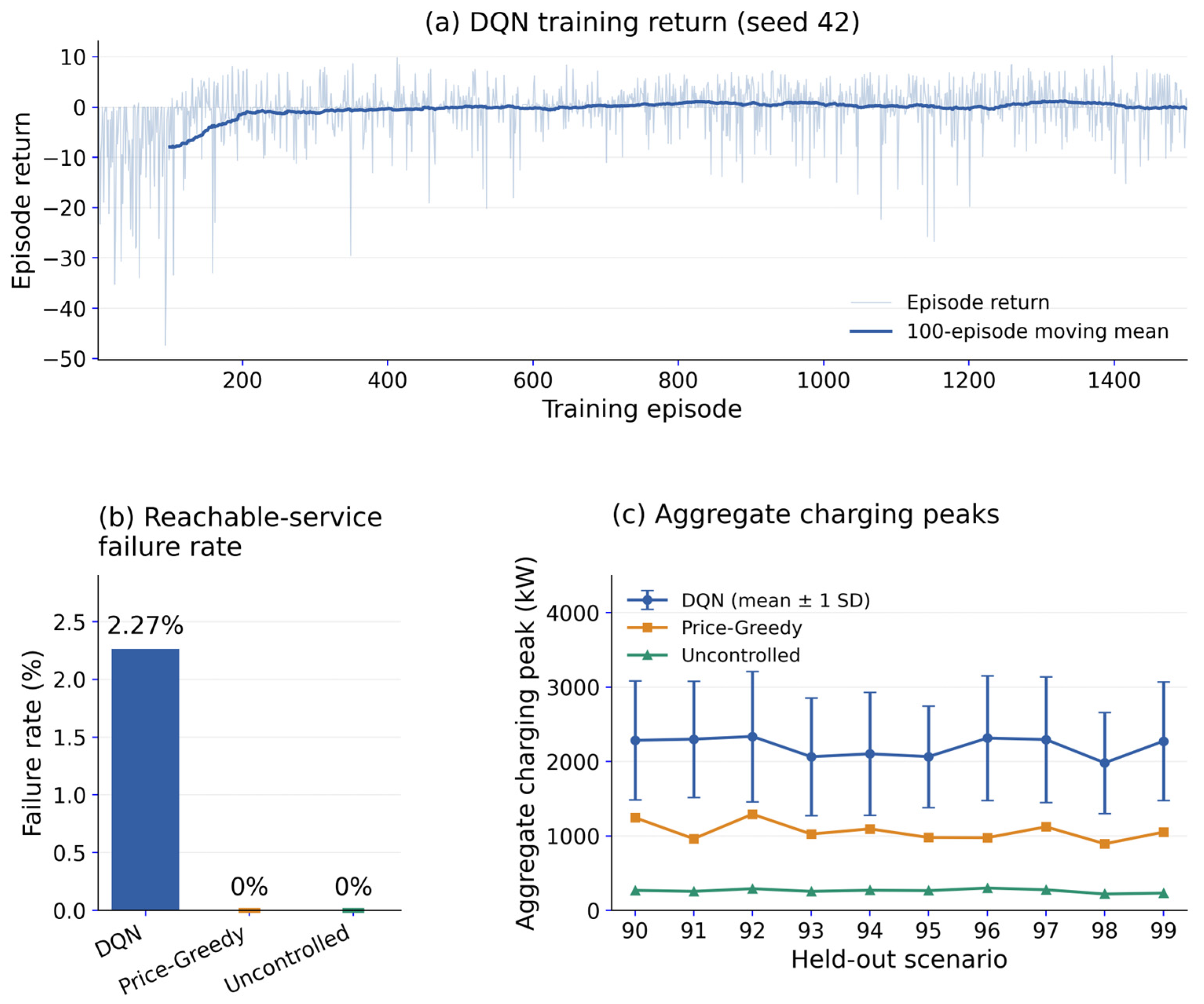
Across ten held-out scenarios and three independently trained DQN seeds, the pooled reachable-service failure rate was 2.27%, whereas the uncontrolled and price-greedy baselines satisfied all reachable service requirements. The DQN achieved a lower weighted charging price but produced substantially higher aggregate peaks, supporting its use as a behavioral reference rather than a directly deployable schedule. Seed 42 training behavior is shown in Figure 5a.

4.2. Stage 1 Headroom and Feasibility Limitation of the RL Profile

The first optimization stage calculates the non-EV baseline operation and determines the remaining headroom available for EV charging. This step is essential because the EV parking lot does not operate in isolation. The available capacity for EV charging depends on the baseline grid load already occupying the connection capacity.

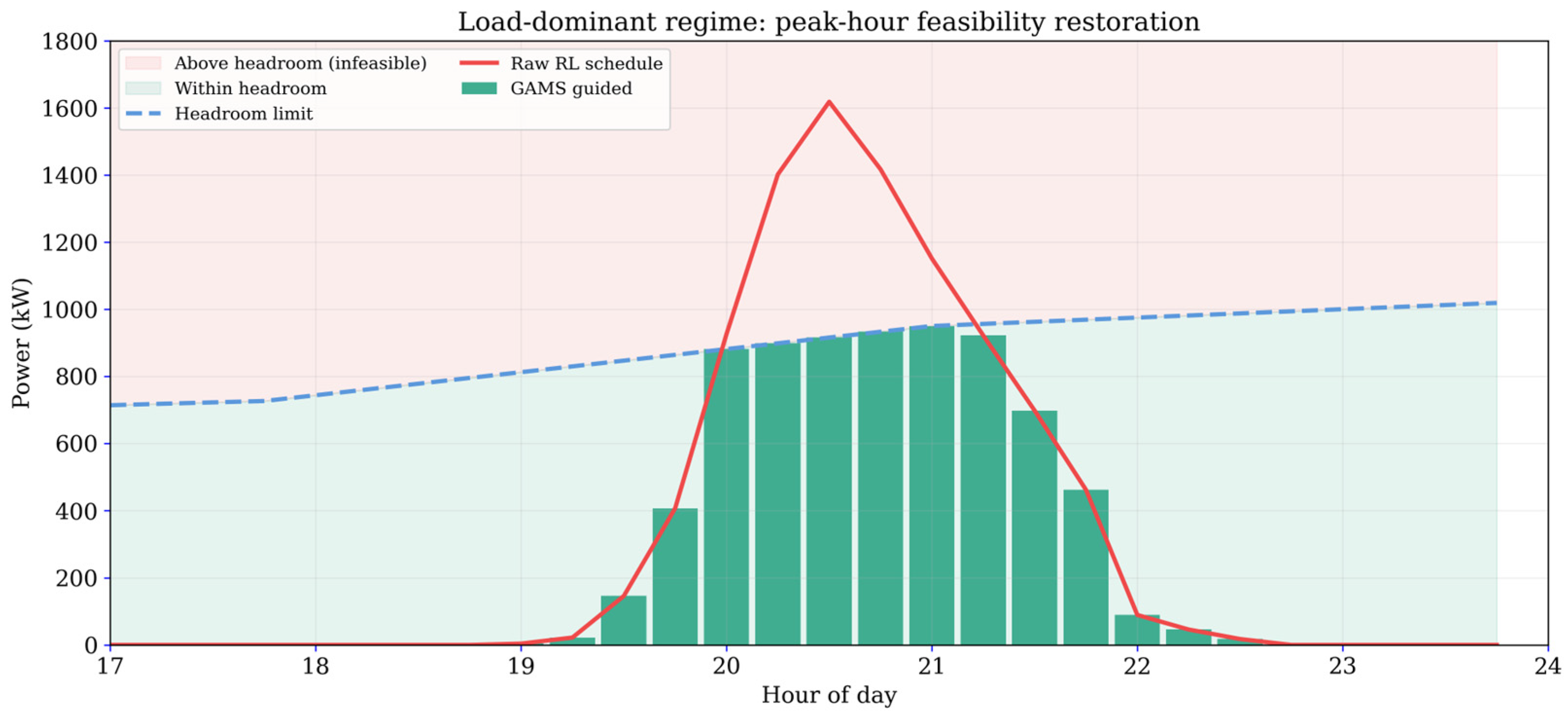
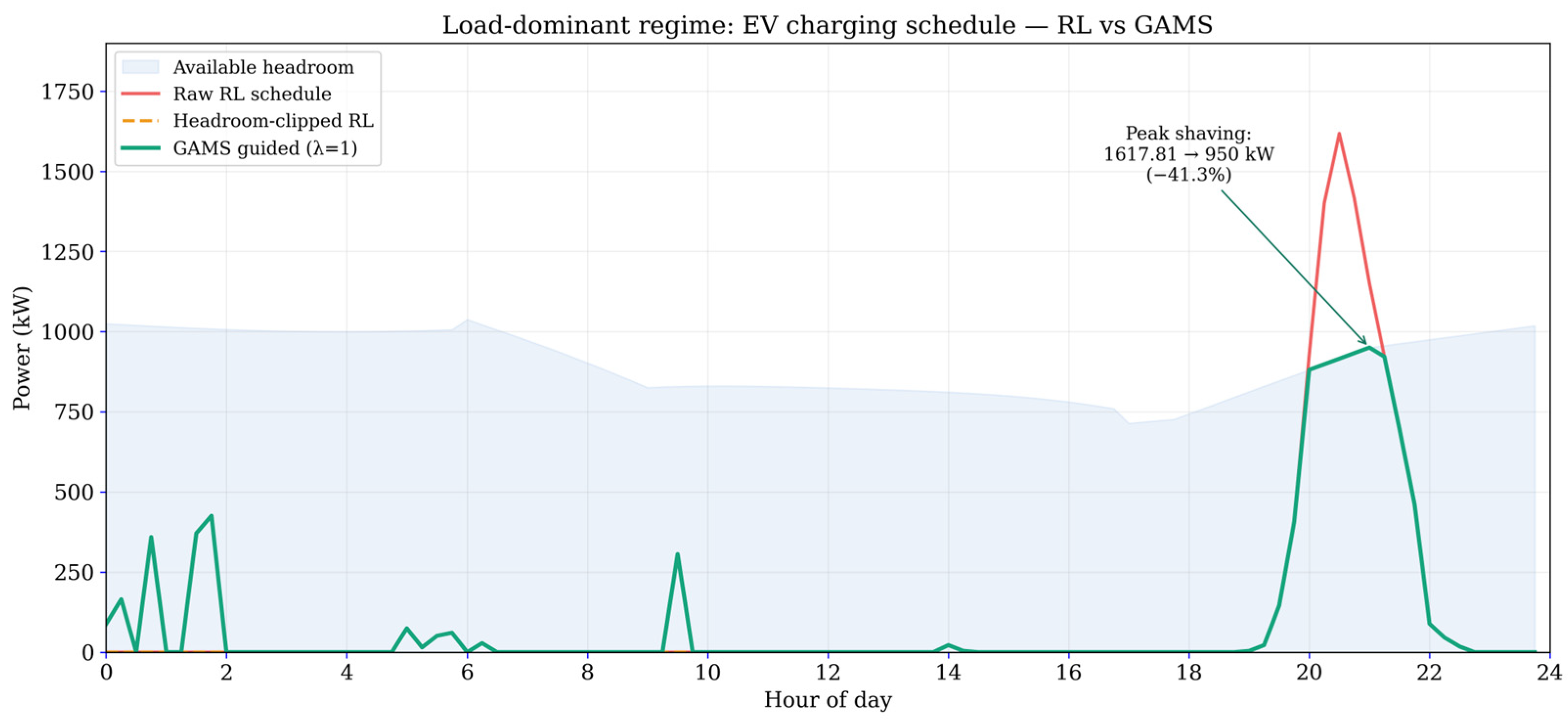
The Stage 1 result shows that the available EV charging headroom changes over time. During critical periods, the remaining headroom is considerably lower than the RL charging demand. At the point of greatest overshoot, the available headroom is 915.60 kW, while the RL profile requires 1617.81 kW. This creates an instantaneous overshoot of 702.21 kW.

The energy removed by naive headroom clipping over the day is 483.66 kWh. This result confirms that the RL-only schedule cannot be applied directly as a physically feasible dispatch schedule. Even though the RL agent performs well at the vehicle-session level, the aggregate profile violates the grid-capacity envelope when it is evaluated against the Stage 1 headroom.

Figure 6 compares the raw RL profile with the headroom-constrained scheduling envelope.

The two-stage structure corrects this issue by limiting Stage 2 grid import according to the residual capacity obtained from Stage 1. As a result, the optimized schedule avoids the infeasible RL peak and redistributes EV charging over the available time intervals.

4.3. RL-Guided Optimized Schedule

After the headroom limitation is introduced, the Stage 2 model redistributes EV charging across the available intervals. The departure-service requirement includes vehicles still connected at the end of the scheduling horizon. The resulting schedule preserves part of the learned temporal structure but removes the infeasible portion of the RL demand identified in Section 4.2. Compared with the RL-only profile, the optimized schedule reduces the peak charging stress on the grid. The RL-only peak is 1617.81 kW, while the GAMS-guided result is 950 kW. This corresponds to a peak reduction of about 41.3%. The reduction is not achieved by ignoring EV demand, but by redistributing charging in a way that respects the available system capacity.

The energy delivered by the different schedules also shows the correction effect in Figure 7. The raw RL profile corresponds to 2395.75 kWh of EV charging energy. When the raw profile is naively clipped to the available headroom, the headroom-clipped RL profile decreases to 1912.09 kWh. The GAMS-guided schedule delivers 2340.89 kWh while satisfying the active system constraints. The aggregate service shortfall is 78.20 kWh, and the guided schedule recovers 428.80 kWh beyond naive clipping.

The difference between the headroom-clipped RL profile and the optimized schedule indicates that feasibility restoration is not only a clipping operation. The optimizer also reallocates charging according to the cost, carbon, and service terms in the Stage 2 objective.

Table 8. Direct comparison of charging schedules in the load-dominant regime.

Schedule	EV Energy (kWh)	Peak EV Power (kW)	Headroom Violation (kWh)	Tracking Deviation (kWh)	Feasibility
RL only	2395.75	1617.81	483.66	0.00	Headroom violated
Optimization-only (${\lambda }_{\mathrm{R}\mathrm{L}}$ = 0)	2404.27	425.53	0.00	4513.85	Feasible with service shortfall
RL-guided (${\lambda }_{\mathrm{R}\mathrm{L}}$ = 1)	2340.89	950.00	0.00	912.45	Feasible with service shortfall

compares the raw RL reference, optimization-only (${\lambda }_{\mathrm{R}\mathrm{L}}$ = 0), and RL-guided (${\lambda }_{\mathrm{R}\mathrm{L}}$ = 1) schedules for the same held-out scenario 90, seed 42, and load-dominant inputs.

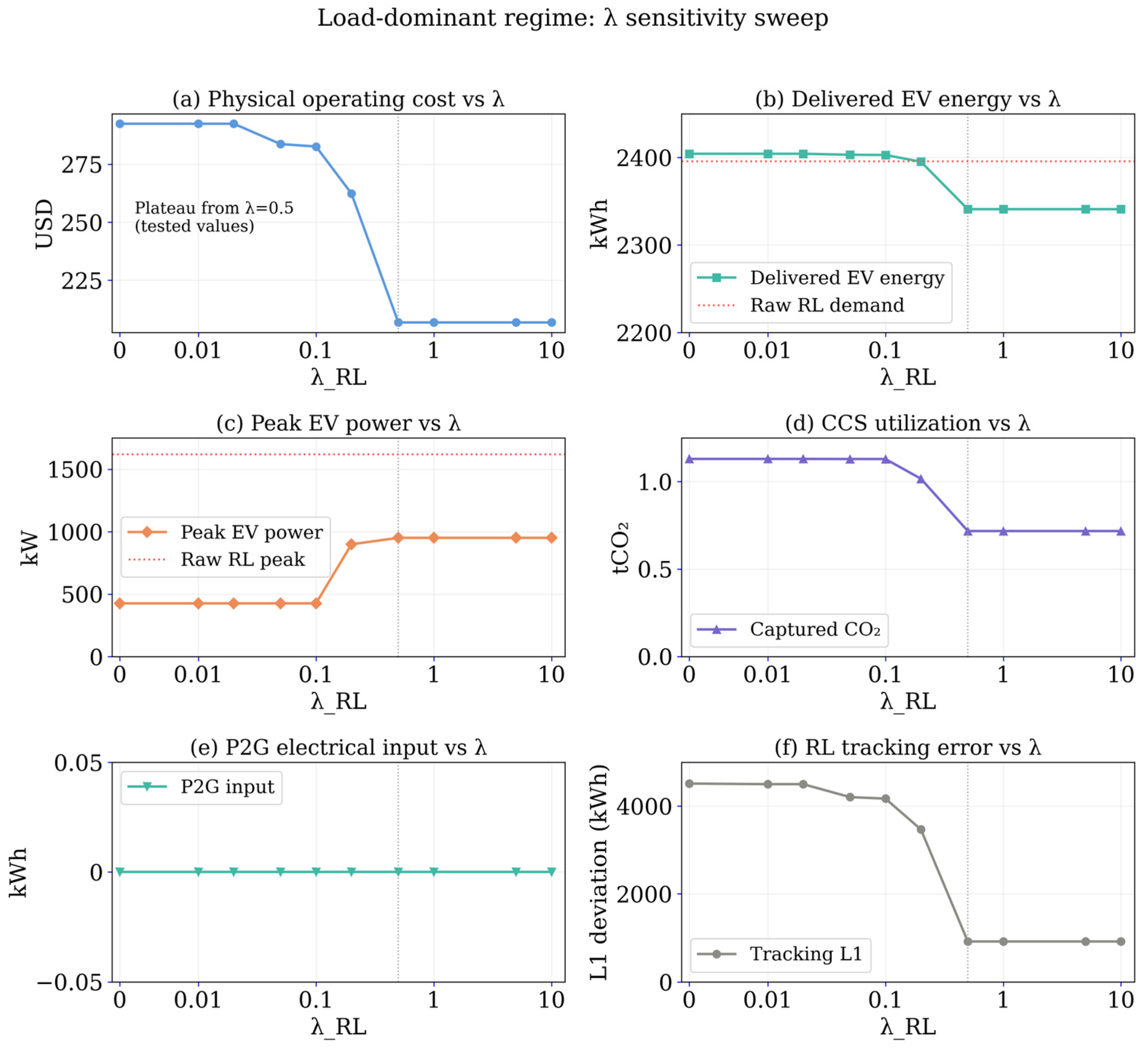
Relative to optimization-only scheduling, DQN guidance reduces the energy-based tracking deviation from 4513.85 to 912.45 kWh (79.8%) in the representative case, showing that the optimized schedule retains substantially more of the learned temporal charging profile.

4.4. Effect of the RL-Tracking Weight

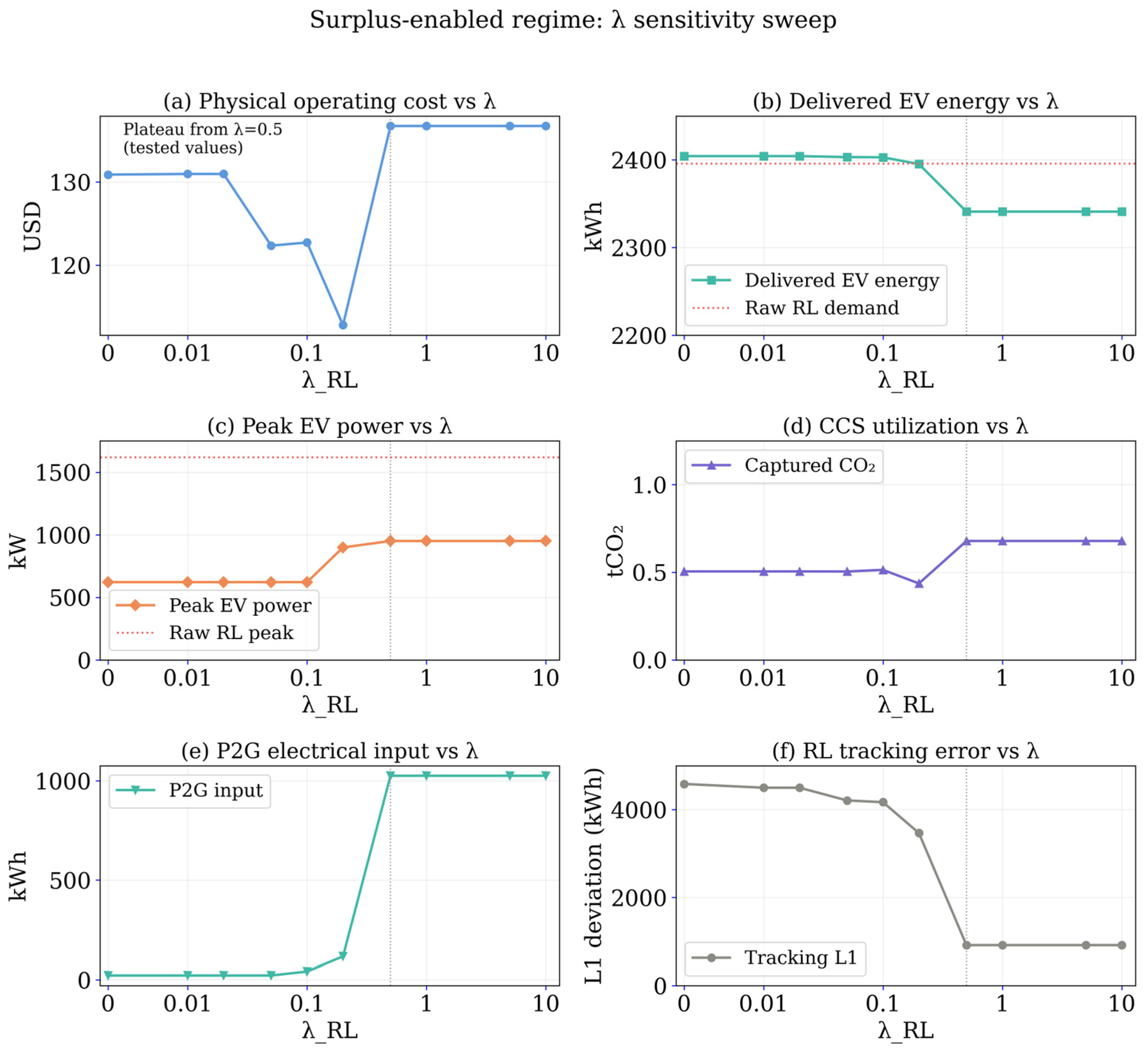
The sweep shows a transition from optimization-dominated to RL-following behavior. At ${\lambda }_{\mathrm{R}\mathrm{L}}$ = 0, the load-dominant solution delivers 2404.27 kWh at a 425.53 kW peak; the corresponding physical costs are 292.44 USD and 130.87 USD in the load-dominant and surplus-enabled regimes, respectively. Increasing ${\lambda }_{\mathrm{R}\mathrm{L}}$ to 0.20 raises the load-dominant peak to 898.45 kW, while delivered energy decreases modestly to 2395.17 kWh. For ${\lambda }_{\mathrm{R}\mathrm{L}}$ ≥ 0.5, the tested solutions reach a plateau at 2340.89 kWh with 912.45 kWh tracking deviation. Further increases in ${\lambda }_{\mathrm{R}\mathrm{L}}$ do not recover the raw RL profile because the remaining deviation is imposed by the system constraints and the joint service, tracking, and operating-cost objective. Figure 8 and Figure 9 summarize these responses for the two operating regimes.

4.5. Multi-Scenario and Multi-Seed Robustness

The scenario SD of service requirement was 150.58 kWh. Delivered-energy scenario SD was 95.6% of this value for RL-guided optimization, compared with 67.7% for headroom clipping (143.93/150.58 and 101.94/150.58, respectively). These ratios compare variability magnitudes, rather than explained variance, and indicate greater responsiveness to fleet-dependent service demand.

Table 9. Multi-scenario robustness in the load-dominant regime across ten held-out fleet scenarios and three DQN seeds.

Method	Metric	Mean	Scenario SD	Seed SD
Headroom-clipped RL reference	EV energy delivered (kWh)	1470.52	101.94	283.81
Headroom-clipped RL reference	Aggregate shortfall (kWh)	743.85	92.88	283.81
Headroom-clipped RL reference	Peak EV power (kW)	938.05	1.25	9.10
RL-guided, ${\lambda }_{\mathrm{R}\mathrm{L}}$ = 1	EV energy delivered (kWh)	2155.87	143.93	17.40
RL-guided, ${\lambda }_{\mathrm{R}\mathrm{L}}$ = 1	Aggregate shortfall (kWh)	58.51	17.77	17.40
RL-guided, ${\lambda }_{\mathrm{R}\mathrm{L}}$ = 1	Peak EV power (kW)	946.82	20.99	7.02

extends the representative scenario 90/seed 42 realization in Section 4.2, Section 4.3 and Section 4.4 to the full held-out panel; the detailed figures and case tables in those sections describe that representative realization.

The optimization layer reduced the seed-to-seed SD of delivered EV energy from 283.81 to 17.40 kWh while increasing mean delivery from 1470.52 to 2155.87 kWh. Seed variability dominates the clipped reference, whereas scenario variability dominates the guided result. The terminal aggregate-stock constraint changes the absolute shortfall but not this variability comparison. The paired surplus-enabled evaluation showed nearly identical variability.

4.6. Role of CCS Under Carbon-Budget Constraint

Within the model, CCS directly affects carbon feasibility because it reduces net emissions after gross grid-related emissions are calculated. In the load-dominant regime, where renewable surplus is not available for P2G, CCS becomes the main multi-energy component that can support additional EV charging when the carbon budget is binding in the electricity-only case.

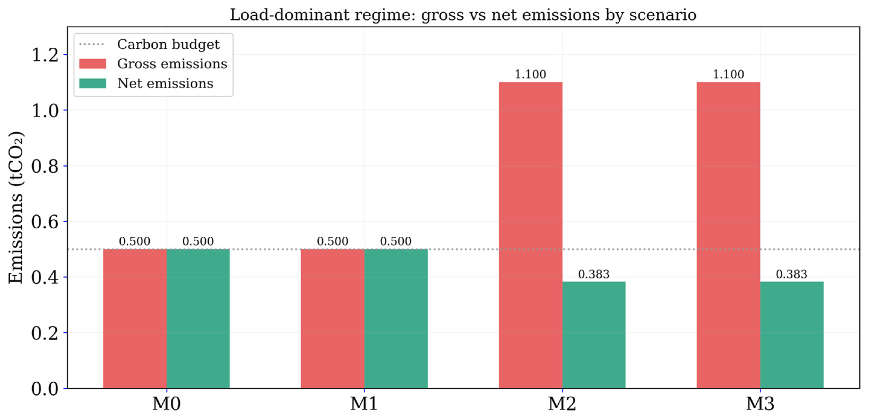
Without CCS, the model delivers 1063.83 kWh of EV charging energy while keeping net emissions at 0.500 tCO₂. With CCS, delivered EV energy increases to 2340.89 kWh. At the same time, CCS captures 0.717673 tCO₂, and net emissions decrease to 0.382546 tCO₂.

For this load-dominant case, the CCS-enabled configuration delivers approximately 120% more EV charging energy than the electricity-only configuration in the modeled comparison while reducing net emissions by about 23.5%. The carbon intensity also decreases from 0.00047 tCO₂/kWh to 0.000163 tCO₂/kWh.

Figure 10 compares gross and net emissions with and without CCS. The figure shows that the gross emission profile alone does not explain the final carbon performance. The net emission after capture is the relevant quantity for evaluating carbon-budget feasibility.

At the baseline emission factor, the 0.50 tCO₂ budget is non-binding with CCS. When the budget is tightened to 0.30 tCO₂, it becomes binding at emission factors of 0.00047 and 0.00065 tCO₂/kWh; under the 0.50 tCO₂ budget, only the highest tested factor is binding. CCS use therefore depends on both the assumed grid-emission factor and the carbon-budget level and is lower in the surplus-enabled regime.

4.7. Role of P2G Under Surplus-Enabled Operation

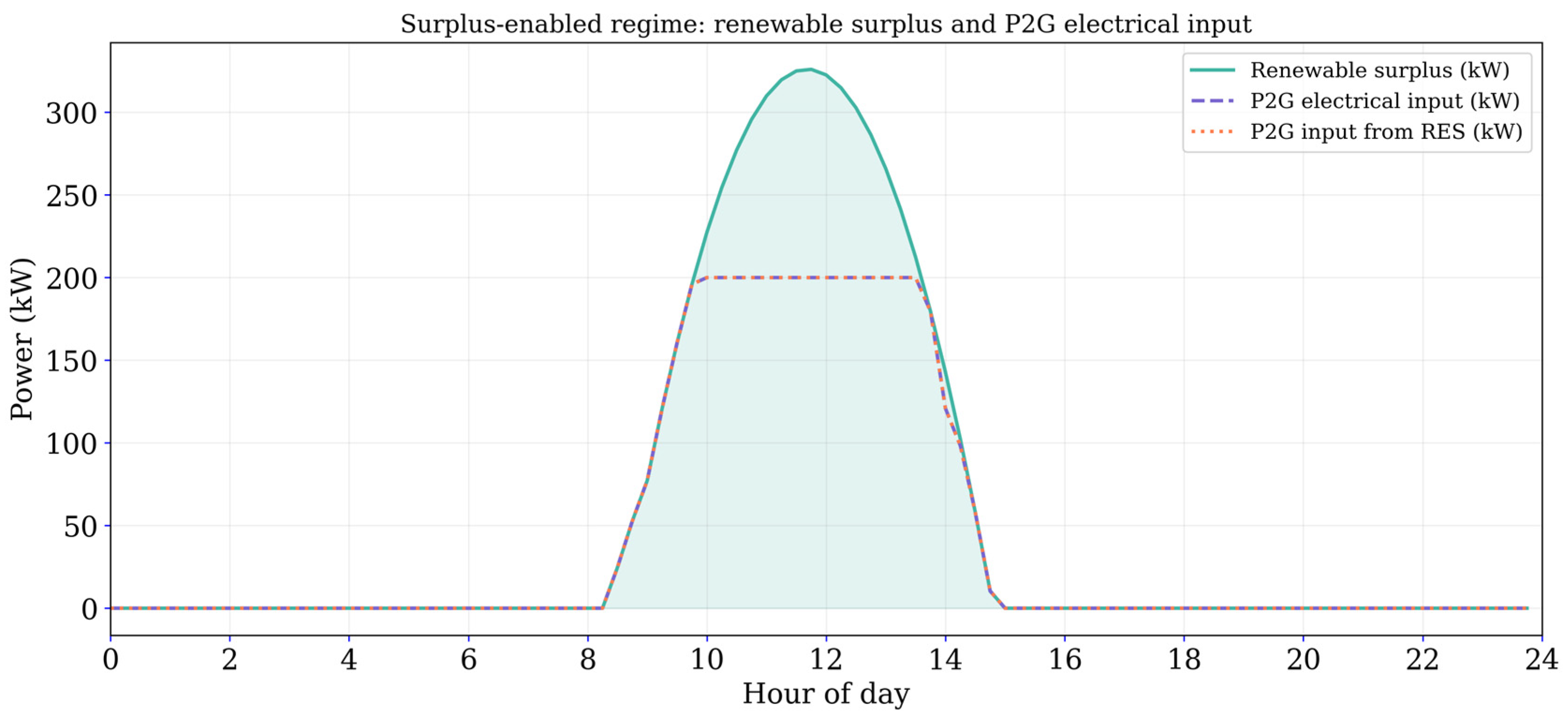
P2G behaves differently from CCS. It does not directly reduce grid-related emissions in the same way as carbon capture. Its role is linked to renewable surplus. Therefore, P2G remains inactive in the load-dominant regime, where no effective surplus is available. It is active only in the surplus-enabled regime. Of the 1351.44 kWh daily renewable surplus, M3 directs 1024.68 kWh to P2G, corresponding to 666.04 kWh of hydrogen energy at ${\eta }_{P2G}$ = 0.65.

This confirms that P2G operates as a surplus-utilization component rather than a general EV-feasibility mechanism. It absorbs renewable energy that would otherwise be exported. Its economic effect is therefore visible mainly in the surplus-enabled regime. Figure 11 confirms that P2G input remains confined to the renewable-surplus window. Relative to M2, adding P2G reduces physical operating cost from USD 159.24 to USD 136.70 (14.2%).

4.8. Comparative Effects of P2G and CCS Across Operating Regimes

The combined configuration comparison separates the roles of electricity-only operation, P2G, CCS, and their joint operation. The results are summarized in

Table 10. Multi-energy configuration comparison.

Regime	Scenario	EV Energy (kWh)	CCS Captured (tCO2)	P2G Input (kWh)	Net Emissions (tCO2)	Physical Operating Cost (USD)
load-dominant	M0	1063.83	0.000000	0.00	0.500000	86.14
load-dominant	M1	1063.83	0.000000	0.00	0.500000	86.14
load-dominant	M2	2340.89	0.717673	0.00	0.382546	206.87
load-dominant	M3	2340.89	0.717673	0.00	0.382546	206.87
Surplus	M0	2370.20	0.000000	0.00	0.500000	87.59
Surplus	M1	2370.20	0.000000	45.07	0.500000	86.59
Surplus	M2	2340.89	0.678663	0.00	0.382546	159.24
Surplus	M3	2340.89	0.678663	1024.68	0.382546	136.70

.

Table 10 shows that P2G changes operating cost without altering EV energy within a fixed CCS state: M0 and M1 have identical EV energy totals, as do M2 and M3. The 2370.20-to-2340.89 kWh difference between the non-CCS and CCS pairs in the surplus-enabled regime reflects re-optimization under the joint tracking, service, cost, and carbon objective; EV energy is not maximized independently. It should therefore be interpreted as a dispatch trade-off rather than an energy penalty caused by CCS. The M2–M3 comparison isolates the incremental economic contribution of P2G.

4.9. Forecast-Error Sensitivity and Perfect-Foresight Limitation

Forecast sensitivity was evaluated for held-out scenario 90 at seed 42 and ${\lambda }_{\mathrm{R}\mathrm{L}}$ = 1 using five paired random draws per operating regime. Mild perturbations applied ±1-step arrival/departure shifts and ±10% changes to initial SoC, baseline load, and renewable generation; stress perturbations used ±2-step timing shifts and ±20% load/renewable changes while retaining ±10% SoC variation. Electricity price and fixed system parameters were unchanged. For each perturbed forecast, the DQN reference and both optimization stages were recomputed, after which the fixed schedule was evaluated against the unperturbed realization without re-optimization. Realizable EV energy was assessed by ex-post clipping, while headroom exceedance was measured before clipping. Paired regime results were not treated as independent statistical replicates.

As summarized in

Table 11. Forecast-error sensitivity results for held-out scenario 90.

Metric	Mild	Stress
Mean EV-energy degradation	2.20% (51.5 kWh)	5.11% (119.6 kWh)
Degradation range	−0.28–4.15%	1.36–9.11%
Mean max headroom exceedance	55.6 kW	120.1 kW
Exceedance range	34.5–63.6 kW	114.0–127.2 kW
Mean violation energy	38.1 kWh	86.9 kWh
Carbon-budget violations	0/5	0/5

, in the load-dominant regime, mean realized EV-energy degradation increased from 2.20% (51.5 kWh) under mild errors to 5.11% (119.6 kWh) under stress errors, while mean maximum headroom exceedance increased from 55.6 to 120.1 kW. Stress degradation exceeded the paired mild case in all five draws; the surplus-enabled regime showed the same trend, with mean degradations of 2.21% and 5.15%. No carbon-budget violation occurred in the tested realizations. These results show that, without an explicit robustness margin, forecast errors at binding intervals can translate into ex-post capacity exceedance and lower realizable EV energy.

Because EV-session variables and system-level load/renewable inputs were perturbed jointly, the reported degradation represents their combined effect. Rolling-horizon re-optimization remains a practical extension.

5. Conclusions

This paper presented an RL-guided two-stage multi-energy optimization framework for carbon-aware EV parking lot charging. A DQN policy was used to generate a charging profile from vehicle-level information, including SoC, time-to-departure, presence, electricity price, and grid-load signals. This profile was then used as a soft reference in a two-stage GAMS model that first determined the residual grid headroom and then scheduled EV charging together with CCS and surplus-linked P2G operation under carbon and capacity constraints.

The results show that the RL profile is useful but not directly feasible at the aggregate system level. The aggregate RL demand reached 1617.81 kW, while the available headroom at the critical interval was 915.60 kW. The RL-guided schedule reduced the peak to 950 kW and delivered 2340.89 kWh under active constraints. The λ_RL analysis showed a trade-off between optimization freedom and behavioral fidelity: the energy-based tracking deviation decreased from 4513.85 kWh at λ_RL = 0 to 912.45 kWh at λ_RL = 1, while the tested solutions reached an RL-following plateau for λ_RL ≥ 0.5. Under carbon-constrained operation, CCS increased delivered EV energy from 1063.83 kWh to 2340.89 kWh and reduced net emissions from 0.500 tCO₂ to 0.383 tCO₂. In the surplus-enabled regime, P2G converted 1024.68 kWh of renewable surplus and reduced the physical cost from USD 159.24 in M2 to USD 136.70 in M3.

The findings indicate that carbon-aware EV parking lot scheduling should be evaluated as a coupled grid, behavior, and multi-energy problem. CCS and P2G contribute through different mechanisms: CCS supports carbon-budget feasibility, while P2G provides surplus-utilization value when renewable excess is present. The proposed framework makes these effects visible by placing the learned charging profile inside an explicit headroom- and carbon-constrained optimization model.

References

1. Mukherjee, J.C.; Gupta, A. A Review of Charge Scheduling of Electric Vehicles in Smart Grid. IEEE Syst. J. 2015, 9, 1541–1553. [Google Scholar] [CrossRef] [Scilit]
2. Amin, A.; Tareen, W.U.K.; Usman, M.; Ali, H.; Bari, I.; Horan, B.; Mekhilef, S.; Asif, M.; Ahmed, S.; Mahmood, A. A Review of Optimal Charging Strategy for Electric Vehicles under Dynamic Pricing Schemes in the Distribution Charging Network. Sustainability 2020, 12, 10160. [Google Scholar] [CrossRef] [Scilit]
3. Binding, C.; Sundstrom, O. Flexible Charging Optimization for Electric Vehicles Considering Distribution Grid Constraints. IEEE Trans. Smart Grid 2012, 3, 26–37. [Google Scholar] [CrossRef] [Scilit]
4. Rotering, N.; Ilić, M. Optimal Charge Control of Plug-In Hybrid Electric Vehicles in Deregulated Electricity Markets. IEEE Trans. Power Syst. 2011, 26, 1021–1029. [Google Scholar] [CrossRef] [Scilit]
5. Limmer, S. Evaluation of Optimization-Based EV Charging Scheduling with Load Limit in a Realistic Scenario. Energies 2019, 12, 4730. [Google Scholar] [CrossRef] [Scilit]
6. Cheng, K.-W.; Bian, Y.; Shi, Y.; Chen, Y. Carbon-Aware EV Charging. In Proceedings of the 2022 IEEE International Conference on Communications, Control, and Computing Technologies for Smart Grids (SmartGridComm), Singapore, 25–28 October 2022; pp. 186–192. [Google Scholar] [CrossRef] [Scilit]
7. Hoehne, C.G.; Chester, M.V. Optimizing plug-in electric vehicle and vehicle-to-grid charge scheduling to minimize carbon emissions. Energy 2016, 115, 646–657. [Google Scholar] [CrossRef] [Scilit]
8. IPCC. IPCC Special Report on Carbon Dioxide Capture and Storage; Metz, B., Davidson, O., de Coninck, H.C., Loos, M., Meyer, L.A., Eds.; Cambridge University Press: Cambridge, UK; New York, NY, USA, 2005. [Google Scholar]
9. Faisal, S.; Gao, C. A Comprehensive Review of Integrated Energy Systems Considering Power-to-Gas Technology. Energies 2024, 17, 4551. [Google Scholar] [CrossRef] [Scilit]
10. Zhang, B.; Wu, X.; Ghias, A.M.Y.M.; Chen, Z. Coordinated carbon capture systems and power-to-gas dynamic economic energy dispatch strategy for electricity–gas coupled systems considering system uncertainty: An improved soft actor–critic approach. Energy 2023, 271, 126965. [Google Scholar] [CrossRef] [Scilit]
11. Pantoš, M. Stochastic optimal charging of electric-drive vehicles with renewable energy. Energy 2011, 36, 6567–6576. [Google Scholar] [CrossRef] [Scilit]
12. Zhao, J.; Wang, J.; Xu, Z.; Wang, C.; Wan, C.; Chen, C. Distribution Network Electric Vehicle Hosting Capacity Maximization: A Chargeable Region Optimization Model. IEEE Trans. Power Syst. 2017, 32, 4119–4130. [Google Scholar] [CrossRef] [Scilit]
13. Zou, S.; Ma, Z.; Liu, X.; Hiskens, I.A. An Efficient Game for Coordinating Electric Vehicle Charging. IEEE Trans. Autom. Control 2017, 62, 2374–2389. [Google Scholar] [CrossRef] [Scilit]
14. Tan, B.; Lin, Z.; Zheng, X.; Xiao, F.; Wu, Q.; Yan, J. Distributionally robust energy management for multi-microgrids with grid-interactive EVs considering the multi-period coupling effect of user behaviors. Appl. Energy 2023, 350, 121770. [Google Scholar] [CrossRef] [Scilit]
15. Minchala-Ávila, C.; Arévalo, P.; Ochoa-Correa, D. A Systematic Review of Model Predictive Control for Robust and Efficient Energy Management in Electric Vehicle Integration and V2G Applications. Modelling 2025, 6, 20. [Google Scholar] [CrossRef] [Scilit]
16. Wu, C.; Gao, S.; Liu, Y.; Song, T.E.; Han, H. A model predictive control approach in microgrid considering multi-uncertainty of electric vehicles. Renew. Energy 2021, 163, 1385–1396. [Google Scholar] [CrossRef] [Scilit]
17. Hermans, B.A.L.M.; Walker, S.; Ludlage, J.H.A.; Özkan, L. Model predictive control of vehicle charging stations in grid-connected microgrids: An implementation study. Appl. Energy 2024, 368, 123210. [Google Scholar] [CrossRef] [Scilit]
18. Zhao, Z.; Lee, C.K.M.; Yan, X.; Wang, H. Reinforcement learning for electric vehicle charging scheduling: A systematic review. Transp. Res. Part E Logist. Transp. Rev. 2024, 190, 103698. [Google Scholar] [CrossRef] [Scilit]
19. Qiu, D.; Wang, Y.; Hua, W.; Strbac, G. Reinforcement learning for electric vehicle applications in power systems: A critical review. Renew. Sustain. Energy Rev. 2023, 173, 113052. [Google Scholar] [CrossRef] [Scilit]
20. Sutton, R.S.; Barto, A.G. Reinforcement Learning: An Introduction, 2nd ed.; The MIT Press: Cambridge, MA, USA, 2018. [Google Scholar]
21. Watkins, C.J.C.H.; Dayan, P. Q-learning. Mach. Learn. 1992, 8, 279–292. [Google Scholar] [CrossRef] [Scilit]
22. Mnih, V.; Kavukcuoglu, K.; Silver, D.; Rusu, A.A.; Veness, J.; Bellemare, M.G.; Graves, A.; Riedmiller, M.; Fidjeland, A.K.; Ostrovski, G.; et al. Human-level control through deep reinforcement learning. Nature 2015, 518, 529–533. [Google Scholar] [CrossRef] [Scilit] [PubMed]
23. Wan, Z.; Li, H.; He, H.; Prokhorov, D. Model-Free Real-Time EV Charging Scheduling Based on Deep Reinforcement Learning. IEEE Trans. Smart Grid 2019, 10, 5246–5257. [Google Scholar] [CrossRef] [Scilit]
24. Sadeghianpourhamami, N.; Deleu, J.; Develder, C. Definition and Evaluation of Model-Free Coordination of Electrical Vehicle Charging With Reinforcement Learning. IEEE Trans. Smart Grid 2020, 11, 203–214. [Google Scholar] [CrossRef] [Scilit]
25. García, J.; Fernández, F. A Comprehensive Survey on Safe Reinforcement Learning. J. Mach. Learn. Res. 2015, 16, 1437–1480. [Google Scholar]
26. Gu, S.; Yang, L.; Du, Y.; Chen, G.; Walter, F.; Wang, J.; Knoll, A. A Review of Safe Reinforcement Learning: Methods, Theories, and Applications. IEEE Trans. Pattern Anal. Mach. Intell. 2024, 46, 11216–11235. [Google Scholar] [CrossRef] [Scilit] [PubMed]
27. Li, H.; Wan, Z.; He, H. Constrained EV Charging Scheduling Based on Safe Deep Reinforcement Learning. IEEE Trans. Smart Grid 2020, 11, 2427–2439. [Google Scholar] [CrossRef] [Scilit]
28. Paraskevas, A.; Aletras, D.; Chrysopoulos, A.; Marinopoulos, A.; Doukas, D.I. Optimal Management for EV Charging Stations: A Win–Win Strategy for Different Stakeholders Using Constrained Deep Q-Learning. Energies 2022, 15, 2323. [Google Scholar] [CrossRef] [Scilit]
29. Wu, F.; Sioshansi, R. A two-stage stochastic optimization model for scheduling electric vehicle charging loads to relieve distribution-system constraints. Transp. Res. Part B Methodol. 2017, 102, 55–82. [Google Scholar] [CrossRef] [Scilit]
30. Soroudi, A. Power System Optimization Modeling in GAMS; Springer: Cham, Switzerland, 2017. [Google Scholar] [CrossRef] [Scilit]
31. Hawkes, A.D. Estimating marginal CO2 emissions rates for national electricity systems. Energy Policy 2010, 38, 5977–5987. [Google Scholar] [CrossRef] [Scilit]
32. Elenes, A.G.N.; Williams, E.; Hittinger, E.; Goteti, N.S. How Well Do Emission Factors Approximate Emission Changes from Electricity System Models? Environ. Sci. Technol. 2022, 56, 14701–14712. [Google Scholar] [CrossRef] [Scilit] [PubMed]
33. Sukprasert, T.; Bashir, N.; Souza, A.; Irwin, D.; Shenoy, P. On the Implications of Choosing Average versus Marginal Carbon Intensity Signals on Carbon-aware Optimizations. In Proceedings of the 15th ACM International Conference on Future and Sustainable Energy Systems (e-Energy ’24), Singapore, 4–7 June 2024; Association for Computing Machinery: New York, NY, USA, 2024; pp. 422–427. [Google Scholar] [CrossRef] [Scilit]
34. Alikhani, P.; Brinkel, N.; Schram, W.; Lampropoulos, I.; van Sark, W. Multi-objective optimization of electric vehicle charging considering market coupling in north-western Europe. Transp. Res. D Transp. Environ. 2025, 146, 104829. [Google Scholar] [CrossRef] [Scilit]
35. Chen, W.; Zhang, J.; Li, F.; Zhang, R.; Qi, S.; Li, G.; Wang, C. Low Carbon Economic Dispatch of Integrated Energy System Considering Power-to-Gas Heat Recovery and Carbon Capture. Energies 2023, 16, 3472. [Google Scholar] [CrossRef] [Scilit]
36. Ma, Y.; Wang, H.; Hong, F.; Yang, J.; Chen, Z.; Cui, H.; Feng, J. Modeling and optimization of combined heat and power with power-to-gas and carbon capture system in integrated energy system. Energy 2021, 236, 121392. [Google Scholar] [CrossRef] [Scilit]
37. EPİAŞ. Turkey Electricity Market Prices. 2025. Available online: https://enerji.gov.tr/evced-cevre-ve-iklim-elektrik-uretim-tuketim-emisyon-faktorleri (accessed on 4 August 2025).
38. Republic of Türkiye Ministry of Energy and Natural Resources. 2023 Türkiye Elektrik Üretimi ve Elektrik Tüketim Noktası Emisyon Faktörleri Bilgi Formu [2023 Türkiye Electricity Generation and Electricity Consumption Point Emission Factors]. Available online: https://enerji.gov.tr/evced-cevre-ve-iklim-elektrik-uretim-tuketim-emisyon-faktorleri (accessed on 11 September 2026).
39. Wang, X.; Star, A.G.; Ahluwalia, R.K. Performance of Polymer Electrolyte Membrane Water Electrolysis Systems: Configuration, Stack Materials, Turndown and Efficiency. Energies 2023, 16, 4964. [Google Scholar] [CrossRef] [Scilit]
Figure 1. Overall structure of the proposed RL-guided two-stage multi-energy optimization framework.
Electronics 15 04294 g001
Figure 2. Two-stage coupling in the load-dominant regime.
Electronics 15 04294 g002
Figure 3. Two-stage coupling in the surplus-enabled regime.
Electronics 15 04294 g003
Figure 4. RL policy charging demand with EV presence.
Electronics 15 04294 g004
Figure 5. Training and held-out evaluation of the DQN charging policy: (a) seed 42 episode return and its 100-episode moving mean, (b) pooled reachable-service failure rate, and (c) aggregate charging peaks across the 10 held-out fleet scenarios. DQN values in panel (c) are means ± 1 SD across seeds 42–44 for each scenario.
Electronics 15 04294 g005
Figure 6. Feasibility restoration in load-dominant regime.
Electronics 15 04294 g006
Figure 7. RL-guided reshaping of EV charging under the headroom constraint.
Electronics 15 04294 g007
Figure 8. Load-dominant regime: λ R L sensitivity; the horizontal axis is linear up to λ R L = 0.01 and logarithmic above.
Electronics 15 04294 g008
Figure 9. Surplus-enabled regime: λ R L sensitivity; the horizontal axis is linear up to λ R L = 0.01 and logarithmic above.
Electronics 15 04294 g009
Figure 10. Load-dominant regime: gross vs. net emissions by scenario.
Electronics 15 04294 g010
Figure 11. Renewable surplus and P2G electrical input in the surplus-enabled regime.
Electronics 15 04294 g011