Comparative Evaluation of Numerical and Symbolic Software Tools for the Simulation and Analysis of Electrical Filters

Abstract

The design and analysis of electrical filters rely on a wide range of numerical and symbolic software environments, each providing different computational and analytical capabilities. However, comprehensive comparative studies that evaluate both approaches using identical filter configurations and common performance criteria remain limited. This paper presents a systematic comparative evaluation of representative active electrical filter structures using SPICE, TINA-TI, MATLAB, MAPLE, ECAP, SYSEG, and TFSYG. The investigated filters are analyzed using a unified methodology based on frequency-domain, time-domain, and symbolic indicators, including magnitude and phase responses, cutoff frequencies, pole-zero distributions, transient responses, and transfer functions. The main contribution is a reproducible cross-platform framework comparing numerical and symbolic environments using equivalent filter models, identical component values, and common analysis criteria. Unlike tool- or topology-specific evaluations, the methodology applies the same comparative procedure to representative active-filter families, distinguishing software-dependent differences from those associated with the underlying circuit model. The results show close agreement for directly comparable quantities while highlighting the complementary capabilities of numerical and symbolic analysis. The proposed methodology provides practical guidelines for selecting appropriate software tools for electrical filter analysis, design, optimization, and engineering education, supporting the combined use of numerical and symbolic techniques in analog circuit development.

1. Introduction

Electrical filters are fundamental building blocks in analog and mixed-signal electronic systems because they enable the selective transmission, attenuation, or suppression of signal components according to frequency. Their accurate design is essential in communication equipment, sensor interfaces, measurement and data-acquisition systems, audio electronics, biomedical instrumentation, and power-electronic applications, where useful information is frequently accompanied by noise, interference, harmonics, or other unwanted spectral components [1,2,3,4]. Recent studies continue to demonstrate the importance of analog filters in communication receivers, integrated sensor interfaces, reconfigurable electronic systems, and electronically tunable signal-processing circuits.

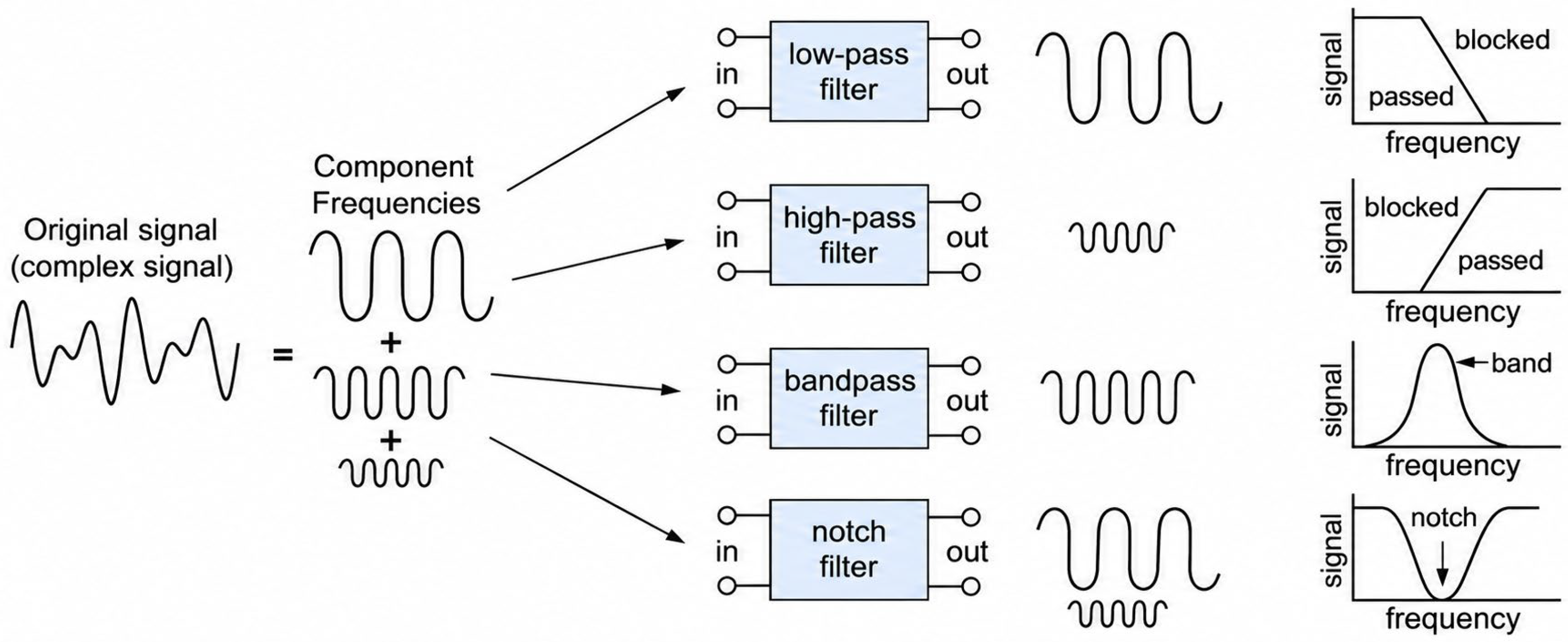
Depending on their frequency-selective behavior, electrical filters are commonly classified as low-pass, high-pass, band-pass, or band-stop filters. Low-pass filters preserve spectral components below a specified cutoff frequency, whereas high-pass filters transmit components above this limit. Band-pass filters select a finite frequency interval, while band-stop filters attenuate a prescribed frequency range. A band-stop structure with a narrow rejection interval is generally referred to as a notch filter [5,6,7]. These basic frequency-selective characteristics are illustrated schematically in Figure 1.

Electrical filters may also be classified according to their circuit implementation. Passive filters are realized exclusively using resistors, capacitors, and inductors, whereas active filters additionally employ active devices, such as operational amplifiers, operational transconductance amplifiers, current conveyors, or current-feedback operational amplifiers. Active implementations are particularly attractive at low and medium frequencies because they can provide gain, buffering, high input impedance, and low output impedance while avoiding the use of bulky inductors. Consequently, active-RC and related filter configurations remain widely investigated for integrated, tunable, and application-specific signal-processing systems [9,10,11,12]. Recent implementations include voltage-mode and current-mode universal filters, switched-capacitor structures, digitally tunable $G_m$-C filters, and active filters designed for sensor interfaces [2,10,11,12].

The performance of a filter is primarily described by its transfer function and the corresponding frequency- and time-domain responses. In the frequency domain, the magnitude response indicates the attenuation or amplification introduced at each frequency, while the phase response describes the phase displacement between the input and output signals. These quantities are commonly represented using Bode diagrams, whereas Nyquist diagrams and pole-zero maps provide complementary information concerning dynamic behavior and stability. In the time domain, transient analysis is used to evaluate waveform distortion, settling behavior, overshoot, delay, and the preservation of the input-signal shape [5].

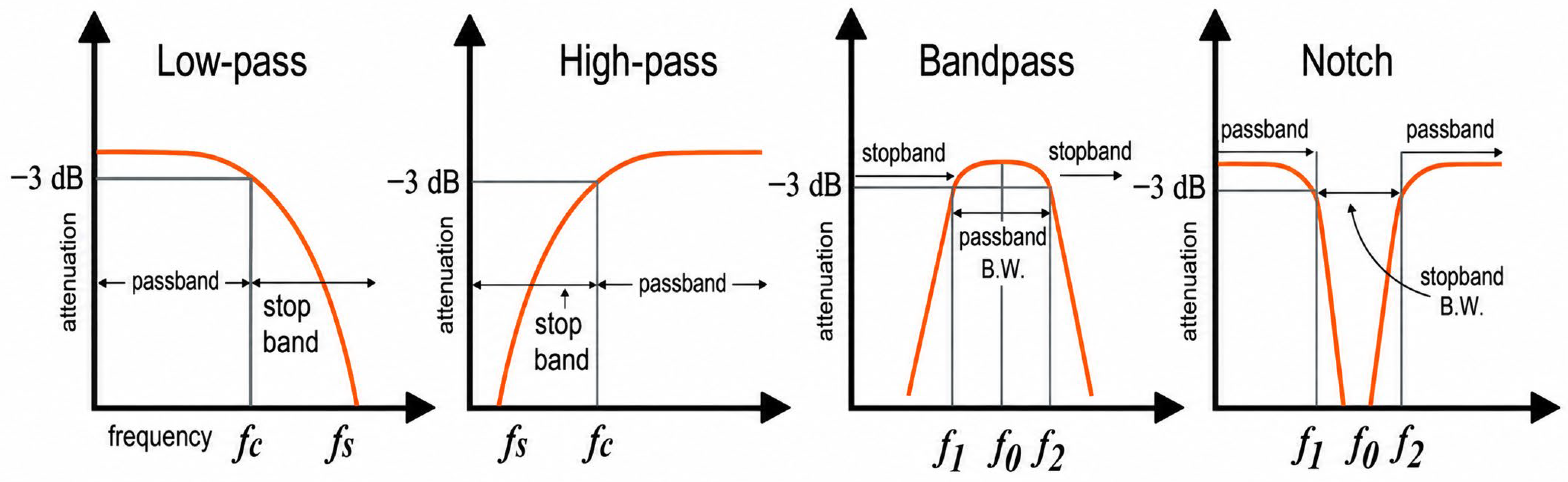
Typical magnitude-response characteristics for the four principal filter categories are shown in Figure 2. The passband defines the frequency range transmitted with an acceptable gain variation, the stopband corresponds to the range in which signal components are attenuated, and the transition region connects these two intervals [5]. The cutoff frequency is conventionally associated with a magnitude decrease of $3 \mathrm{d}\mathrm{B}$ relative to the passband reference level. For band-pass and band-stop filters, the lower and upper cutoff frequencies are denoted by $f_1$ and $f_2$, respectively, and the bandwidth is expressed as:

$$BW=f_2-f_1.$$

(1)

The center frequency is commonly defined as:

$$f_0=\sqrt{f_1{f}_2},$$

(2)

while the quality factor is given by:

$$Q={\displaystyle \frac{f_0}{BW}}={\displaystyle \frac{f_0}{f_2-f_1}}.$$

(3)

The increasing complexity of analog circuits and the need to evaluate multiple design alternatives have made computer-aided analysis an essential stage of modern filter development. Numerical circuit simulators enable designers to investigate circuit operation before hardware implementation and to evaluate responses under specified excitation, component, and device-model conditions. SPICE-based environments are commonly used for AC, transient, pole-zero, noise, and sensitivity analyses. TINA-TI provides a SPICE-based environment for DC, transient, and frequency-domain circuit analysis and is therefore employed in this study for the numerical evaluation of the investigated active-filter structures [13]. MATLAB is frequently employed for numerical processing, response calculation, graphical representation, and the independent verification of simulation results [14,15,16,17].

Numerical simulation is particularly useful for reproducing practical circuit behavior and for incorporating non-ideal device models, supply conditions, initial states, and excitation waveforms. However, its results are usually provided as numerical values or graphical curves associated with a specific set of component parameters. Consequently, numerical simulation alone may not always reveal the explicit analytical relationships between circuit elements and the resulting transfer characteristics.

Symbolic circuit analysis complements numerical simulation by expressing circuit characteristics as analytical functions of the circuit variables and parameters. Depending on the adopted method and software environment, symbolic analysis may provide transfer functions, characteristic equations, poles, zeros, eigenvalues, and parameter sensitivities. In the present comparative study, the quantitative assessment focuses primarily on frequency responses, cutoff frequencies, transient behavior, transfer functions, and pole-zero characteristics, which are consistently available for the investigated filter configurations. Symbolic expressions can therefore support circuit interpretation, model verification, parameter selection, tolerance analysis, and design optimization [15,16,17,18,19].

The two approaches therefore serve complementary purposes. Numerical tools efficiently calculate circuit responses for assigned component values and device models, whereas symbolic tools reveal the mathematical structure of the analyzed system. Agreement between independently obtained numerical and symbolic results provides an additional means of verifying the circuit model, the selected parameter values, and the implemented analysis procedure [14,15,16,17].

Although numerous studies have addressed synthesis, simulation, optimization, or experimental validation of individual filter topologies, the reported investigations generally concentrate on a specific circuit, a limited family of structures, or a single principal simulation methodology. For example, recent studies have examined universal active filters, digitally tunable filters, switched-capacitor filters, sensor-interface filters, and computer-assisted analog-filter synthesis. However, systematic evaluations that apply several numerical and symbolic software tools to multiple representative active-filter topologies using a common set of performance indicators are less frequently reported [9,10,11,12].

Moreover, results obtained using different software environments are not always presented in a directly comparable form. Some tools emphasize graphical numerical simulation, others provide analytical expressions, and others are developed for specialized symbolic or topological analyses. This diversity makes it difficult to assess whether differences between reported results originate from the circuit model, the numerical procedure, the symbolic formulation, or the graphical representation adopted by each program. A comparative methodology based on identical or equivalent circuit models is therefore useful for evaluating the consistency and complementary capabilities of these tools [20].

Previous studies have demonstrated the effectiveness of numerical simulation and symbolic analysis for active-filter design and verification; however, they generally focus on individual circuit topologies, specific design problems, or a limited number of software environments. Consequently, relatively little direct evidence is available on the equivalence of numerical and symbolic results obtained for the same circuit structures, component values, excitation conditions, and evaluation criteria [9,10,11,12]. Moreover, software-specific modeling and output representations complicate cross-platform evaluation, leaving a methodological gap in the systematic comparison of heterogeneous numerical and symbolic environments under controlled and reproducible conditions.

To address this gap, this study introduces a unified framework for comparing numerical and symbolic analyses of representative active filters. Its novelty lies not in a new filter topology or simulation algorithm, but in applying multiple software environments to equivalent filter implementations with identical component values and common evaluation criteria. This controlled approach distinguishes software-dependent numerical, symbolic, and representational differences from those associated with the circuit model. Unlike studies focused on a single filter family or analysis environment, the framework is consistently applied to low-pass, high-pass, notch, and band-pass filters, integrating frequency-domain, time-domain, transfer-function, and pole-zero results. The included numerical and symbolic input descriptions further support reproducibility and independent verification of the cross-platform comparisons. The investigated examples include a third-order Bessel low-pass filter, a third-order Bessel high-pass filter, second-order notch filters designed for power-line interference suppression at 50 and 60 Hz, a third-order Butterworth high-pass filter, a fifth-order Sallen–Key Bessel low-pass filter, and a band-pass filter intended for voice-communication applications.

The circuits are analyzed using SPICE, TINA-TI, TFSYG, MATLAB, MAPLE, ECAP, SYSEG, and, where required by the symbolic formulation, CSAP. The comparison covers frequency- and time-domain characteristics, including magnitude and phase responses, cutoff frequencies, transient waveforms, Nyquist representations, pole-zero distributions, and transfer functions. Equivalent circuit models are used where required by individual software environments, and the resulting characteristics are compared to assess agreement between numerical and symbolic formulations.

The novelty lies not in the established filter topologies, but in the cross-platform verification methodology. Bessel, Butterworth, notch, and Sallen–Key filters serve as representative cases for assessing the consistency and complementary capabilities of numerical and symbolic environments under comparable modeling conditions.

The principal contributions of this study are summarized as follows:

• A reproducible cross-platform comparison framework is established using equivalent circuit implementations, identical component values, and common evaluation criteria across numerical and symbolic software environments.
• The same methodology is applied to several representative active-filter families, including low-pass, high-pass, notch, and band-pass configurations, rather than being restricted to a single topology.
• Numerical and symbolic results are compared directly using frequency responses, cutoff frequencies, transient characteristics, transfer functions, and pole-zero information, allowing software-dependent differences to be distinguished from circuit-model differences.
• The complementary capabilities and practical limitations of SPICE, TINA-TI, MATLAB, MAPLE, ECAP, SYSEG, TFSYG, and CSAP are evaluated within a common analytical context.
• Numerical and symbolic input descriptions are provided to support reproducibility and independent verification of the comparative procedure.

The objective of this study is not to identify a universally superior software package, since the tools investigated differ in their intended purpose, functionality, and analytical capabilities. Instead, the study aims to evaluate the consistency of the results obtained using equivalent filter models and to demonstrate how numerical simulation and symbolic analysis can be effectively combined for filter analysis, verification, and design.

The remainder of this paper is organized as follows. Section 2 compares the selected active-filter structures using numerical and symbolic analyses of their frequency-domain, time-domain, pole-zero, and transfer-function characteristics. Section 3 presents the conclusions of this study, summarizes the main findings, and highlights the benefits of combining numerical simulation with symbolic analysis for electrical filter evaluation and verification.

2. Simulation and Analysis of Electrical Filter Structures

Complementary numerical and symbolic analyses were performed using SPICE, TINA-TI, MATLAB, MAPLE, ECAP, SYSEG, and TFSYG, according to the capabilities of each software environment. The results were compared in terms of cutoff frequency, frequency response, transient behavior, pole-zero distribution, and transfer-function characteristics [5,6,7,8,9,10].

For the cross-platform comparison, equivalent implementations are defined as circuit models with the same nominal component values, excitation conditions, and target transfer characteristics. Common comparison quantities include cutoff frequency, magnitude and phase responses, transient behavior, transfer functions, and pole-zero locations, according to their availability in each software environment. Where corresponding numerical values are available, agreement is quantified using the relative deviation:

$${\epsilon }_x={\displaystyle \frac{\left|x_{num}-x_{ref}\right|}{\left|x_{ref}\right|}}\times 100\%.$$

(4)

where $x_{\mathrm{n}\mathrm{u}\mathrm{m}}$ denotes the value obtained from the numerical implementation and $x_{\mathrm{r}\mathrm{e}\mathrm{f}}$ denotes the corresponding value obtained from the symbolic or analytical representation.

For gain and phase, the discrepancies between the numerical and symbolic results are expressed as absolute differences:

$$\begin{gathered} ∆G=\left|G_{num}-G_{sym}\right|, \\ ∆\phi =\left|{\phi }_{num}-{\phi }_{sym}\right|. \end{gathered}$$

(5)

where $G_{\mathrm{n}\mathrm{u}\mathrm{m}}$ and $G_{\mathrm{s}\mathrm{y}\mathrm{m}}$ are the gain values obtained from the numerical and symbolic analyses, respectively, while ${\phi }_{\mathrm{n}\mathrm{u}\mathrm{m}}$ and ${\phi }_{\mathrm{s}\mathrm{y}\mathrm{m}}$ are the corresponding phase values. Accordingly, $\Delta G$ is expressed in dB and $\Delta \phi$ in degrees.

For quantities available only graphically, agreement is assessed from the reported plots, and no numerical error is assigned unless corresponding numerical values are available.

The operational-amplifier representation depends on the circuit and software environment. Numerical implementations use device models associated with the original filter configurations, including OPA364 and OPA132, while some SPICE input descriptions use the UA741 macromodel. In symbolic analyses, operational amplifiers are represented by ideal voltage-controlled voltage sources with sufficiently high open-loop gain to obtain tractable analytical expressions. Thus, numerical–symbolic equivalence refers primarily to the intended closed-loop filter characteristics under the considered operating conditions rather than to identical internal transistor-level amplifier representations.

For reproducibility, the software environments used were Cadence PSpice A/D 17.4, TINA-TI 2008, MATLAB R2026a, Maple 18, ECAP 2014, SYSEG 2014, TFSYG 2014, and CSAP 2014. Unless otherwise specified, standard solver and numerical tolerance settings were used; specific analysis parameters are reported with the corresponding circuit descriptions where required. The component values, excitation conditions, analysis ranges, and representative numerical and symbolic input descriptions required to reconstruct the filter models are provided in the main text and Appendix A.

2.1. Third-Order Bessel Low-Pass Filter

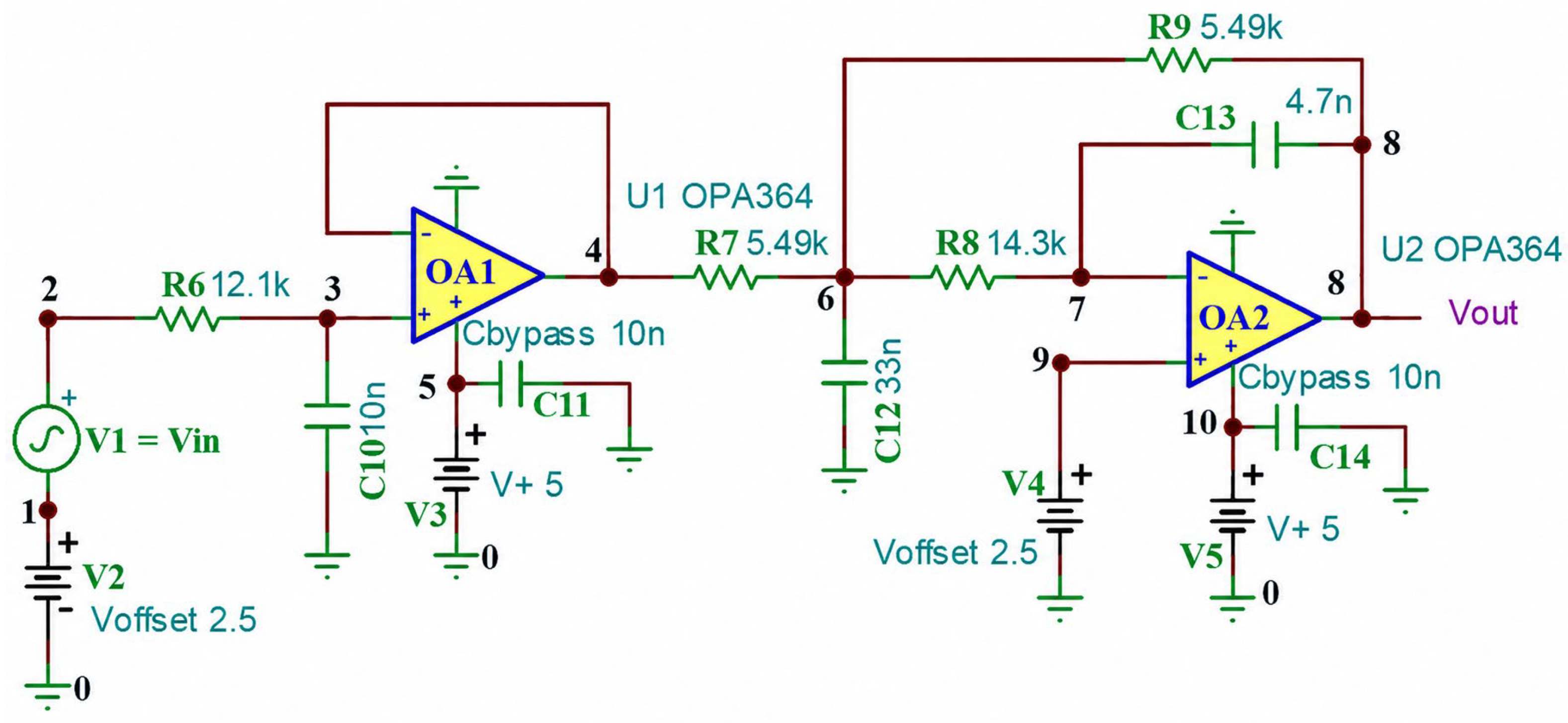
The first circuit considered in this study is a third-order Bessel low-pass filter. Its schematic, generated using the Exe3_LPF.TSC design file, is presented in Figure 3. The circuit was analyzed using the numerical simulation environments SPICE, TINA-TI, and MATLAB together with the symbolic-analysis tools MAPLE, ECAP, SYSEG, and TFSYG. To ensure a fair comparison, identical component values and excitation conditions were employed in all software environments. The corresponding SPICE and symbolic input files are provided in Appendix A.1 for reproducibility purposes.

In the symbolic implementation, the operational amplifiers were modeled as ideal voltage-controlled voltage sources with sufficiently large voltage gains, while their input terminals were represented by ideal current sources. Under these assumptions, the symbolic model produces practically the same responses as the numerical operational-amplifier model, allowing a direct comparison between the two analysis approaches.

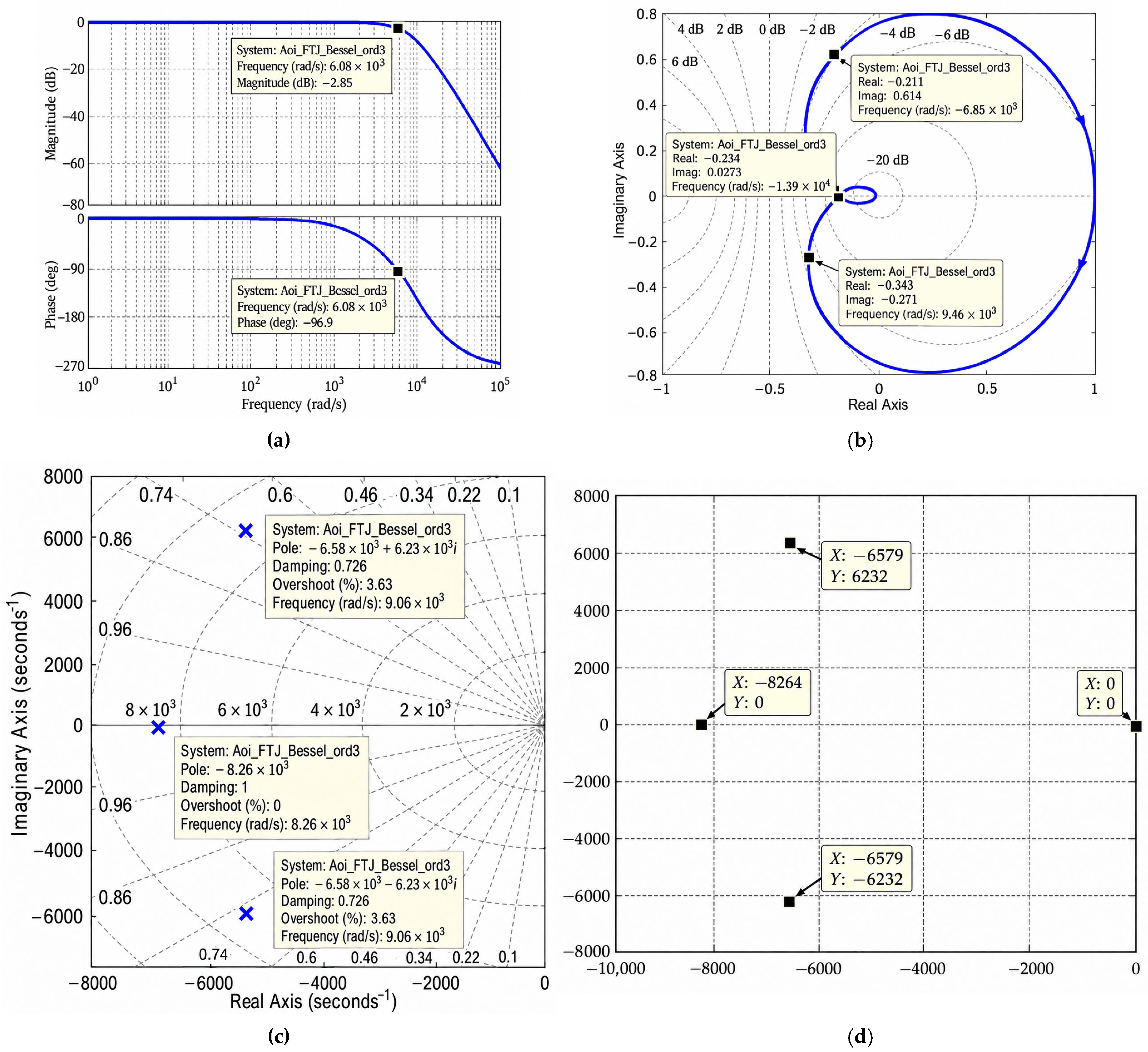
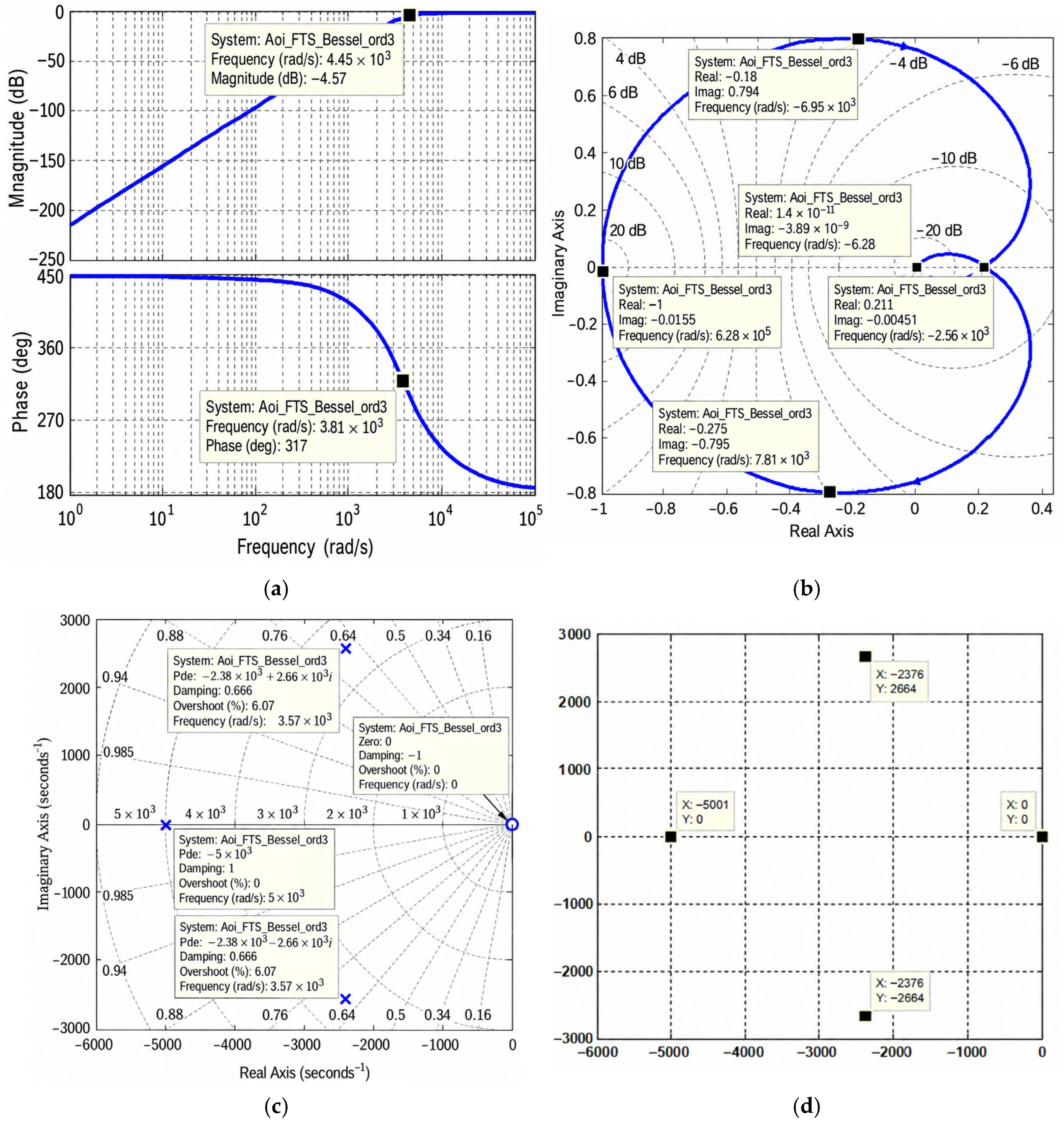
The frequency-domain characteristics obtained for the third-order Bessel low-pass filter are presented in Figure 4. As expected, the Bode diagram exhibits a nearly flat passband followed by a smooth attenuation beyond the cutoff frequency, which is characteristic of the Bessel approximation. Compared with other filter approximations, the transition between the passband and the stopband is more gradual, providing improved phase linearity and group-delay performance.

The Nyquist diagram confirms the expected frequency response of the transfer function without indicating abnormal behavior. Furthermore, the pole-zero map shows that all poles are in the left half of the complex plane, demonstrating that the filter is stable. The symbolic pole-zero representation generated by TFSYG coincides with the numerical results, confirming the consistency of the symbolic-analysis procedure.

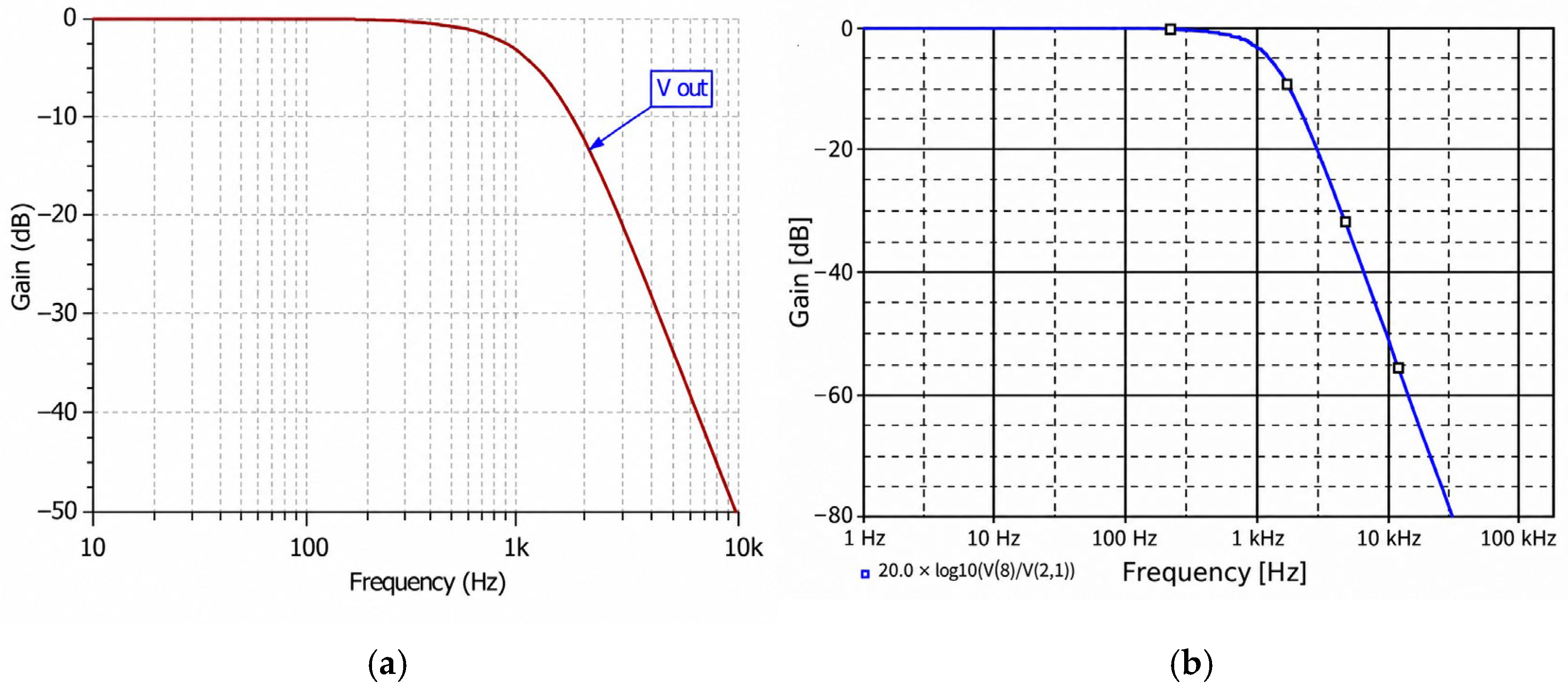
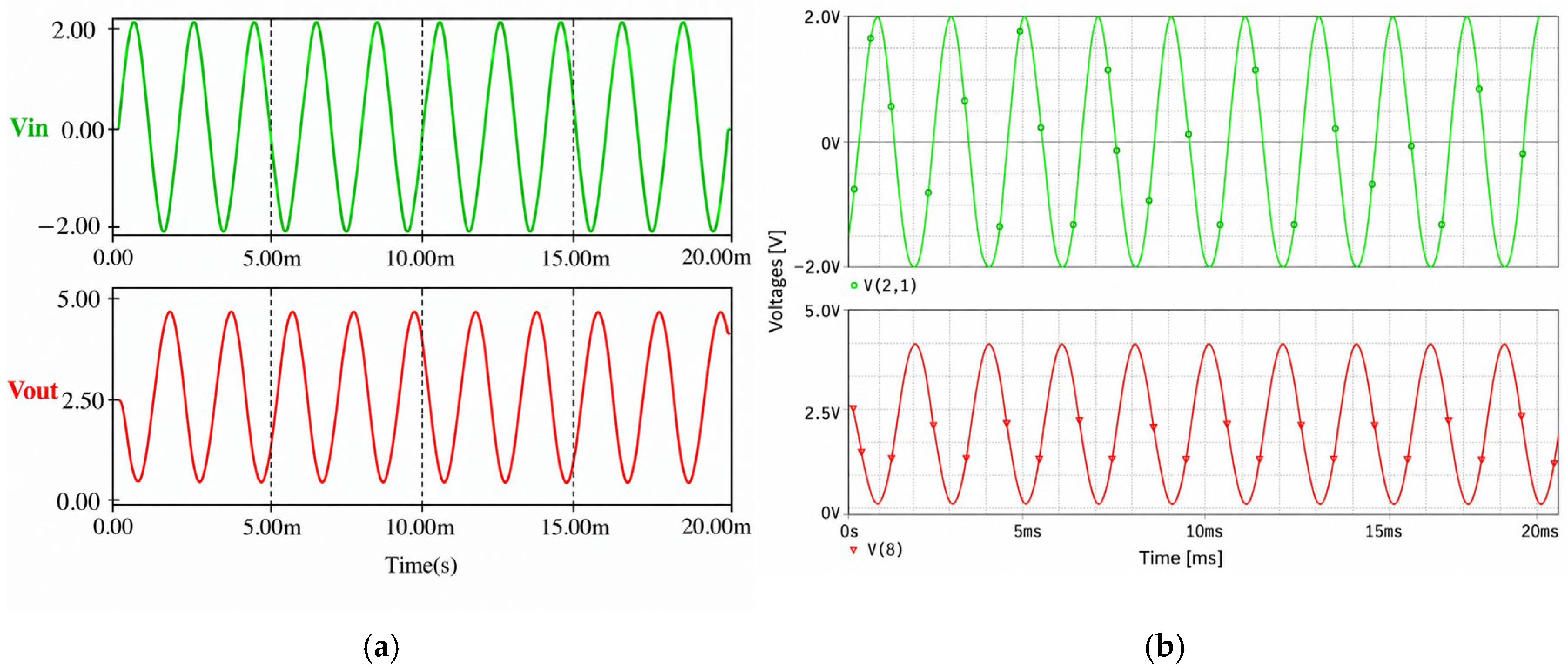
Figure 5 and Figure 6 compare the frequency-domain and time-domain responses, respectively, obtained using the numerical and symbolic simulation environments. These comparisons are used to verify the consistency of the implemented filter models across the investigated software tools.

Figure 5 compares the magnitude responses of the third-order Bessel low-pass filter obtained using TINA-TI and SPICE/TFSYG. Although the graphical interfaces differ in terms of axis formatting, grid density, and visualization style, both software environments produce closely matching frequency responses. The passband remains almost flat up to the cutoff frequency, followed by the characteristic attenuation of a third-order Bessel low-pass filter. The two responses exhibit close agreement over the analyzed frequency range. This observation is further supported by the quantitative analysis presented in Section 2.6.

Figure 6 compares the transient responses obtained using the TINA-TI and SPICE simulation environments. The input and output voltage waveforms exhibit the same time-domain behavior in both cases. Although the graphical layouts differ because of the visualization tools implemented by each software package, the waveform shapes, amplitudes, and phase relationships show close agreement. These results confirm the consistency of the numerical simulations and further validate the analyzed filter model.

The frequency-domain and time-domain comparisons presented in Figure 5 and Figure 6 show consistent behavior between the investigated software environments, while the corresponding quantitative deviations are reported in Section 2.6. The Bode characteristics, pole-zero distributions, and transient responses consistently reproduce the expected behavior of the third-order Bessel low-pass filter. Therefore, both numerical and symbolic analysis tools provide reliable and mutually consistent results for the investigated filter topology.

2.2. Third-Order Bessel High-Pass Filter (HPF) Designed for a Nominal Frequency of 1 kHz

The second circuit analyzed in this study is a third-order Bessel high-pass filter designed for a nominal frequency of 1 kHz. This value represents the nominal design frequency used for the filter configuration and should be distinguished from the cutoff frequency determined from the simulated magnitude response. For consistency with the quantitative comparison adopted in this study, the cutoff frequency, $f_c$, is defined as the frequency corresponding to the −3.0103 dB level relative to the passband gain. According to this criterion, the cutoff frequency obtained for the implemented third-order Bessel high-pass filter is 867.54 Hz, as reported in Section 2.6. The circuit schematic, generated using the Exe3_HPF.TSC design file, is presented in Figure 7. The filter was analyzed using identical circuit configurations in the SPICE, TINA-TI, MATLAB, MAPLE, ECAP, SYSEG, and TFSYG software environments. To support reproducibility, the corresponding numerical and symbolic input descriptions are provided in Appendix A.2.

As in the previous example, the operational amplifier was represented in the symbolic model by an ideal voltage-controlled voltage source with a sufficiently high voltage gain. This approximation produces practically the same response as the numerical operational-amplifier model, allowing a direct comparison between numerical and symbolic simulation approaches.

The frequency-domain characteristics of the third-order Bessel high-pass filter are presented in Figure 8. The Bode diagram exhibits the expected high-pass behavior, with strong attenuation at low frequencies and a nearly constant gain above the cutoff frequency. Compared with higher-selectivity approximations, the Bessel response provides a smoother transition while preserving favorable phase linearity.

The Nyquist diagram confirms the expected frequency response of the transfer function without indicating unstable behavior. Furthermore, the pole-zero map shows that all poles are in the left half of the complex plane, demonstrating that the filter is stable. The symbolic pole-zero representation obtained with TFSYG agrees with the numerical results, confirming the consistency of the symbolic-analysis procedure.

Figure 9 compares the magnitude responses obtained using the TINA-TI and SPICE/TFSYG environments. Although the graphical representations differ because of the visualization tools implemented by each software package, both responses exhibit closely matching high-pass characteristics. The gain increases in the transition region and remains approximately constant within the passband. The close agreement between the responses supports the consistency of the numerical and symbolic simulation environments.

The frequency-domain and time-domain comparisons presented in Figure 8 and Figure 9 show close agreement between the investigated software environments. All numerical and symbolic analyses consistently reproduce the expected characteristics of the third-order Bessel high-pass filter, including the magnitude response, pole-zero distribution, stability, and transient behavior. These results confirm that both numerical simulation and symbolic analysis provide reliable and complementary tools for the analysis and verification of analog high-pass filter circuits.

2.3. Second-Order Notch Filters for Power-Line Interference Suppression

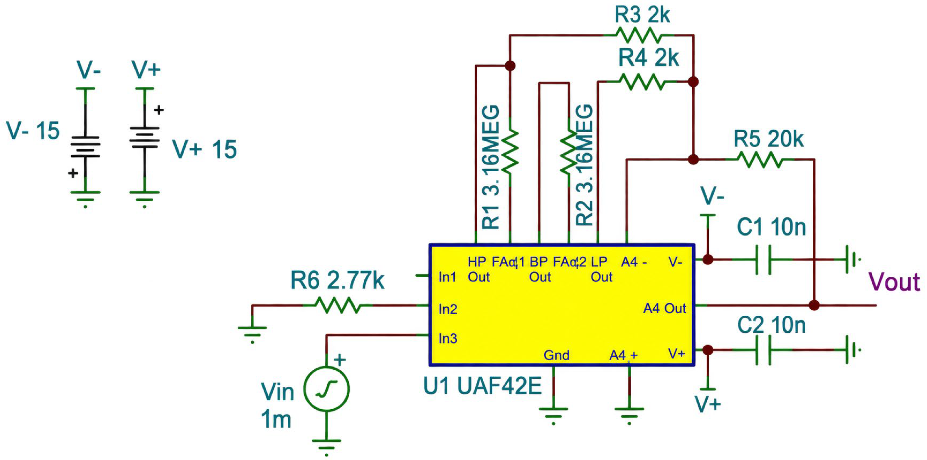
Power-line interference is one of the most common sources of low-frequency noise in analog measurement and communication systems. Depending on the geographical region, the interference frequency is typically 50 Hz or 60 Hz. Therefore, two second-order notch filters were analyzed to evaluate their capability to suppress the corresponding mains-frequency components while preserving the remaining signal spectrum. Two second-order notch-filter implementations were considered for this purpose. The 50 Hz configuration employs the UAF42 universal active filter, whereas the 60 Hz configuration is implemented using discrete RC networks and OPA132 operational amplifiers (Texas Instruments, Dallas, TX, USA). The two circuits therefore serve the same functional objective of power-line interference suppression but employ different circuit implementations.

Figure 10 presents the schematic of the second-order notch filter designed for 50 Hz interference suppression. The circuit employs the UAF42 universal active filter configured in band-stop mode [21]. External resistors are used to adjust the notch frequency, whereas the integrated precision capacitors ensure accurate frequency tuning and improved long-term stability.

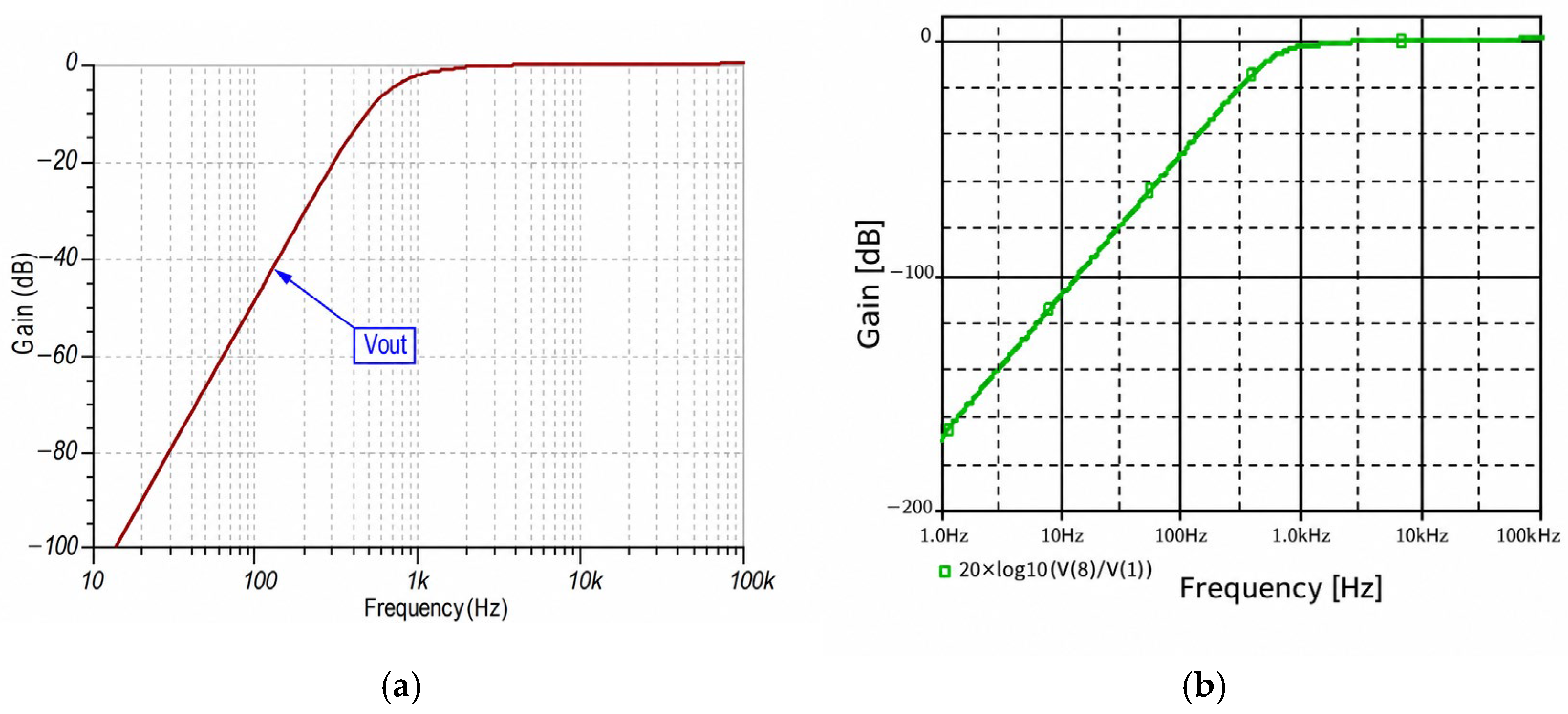
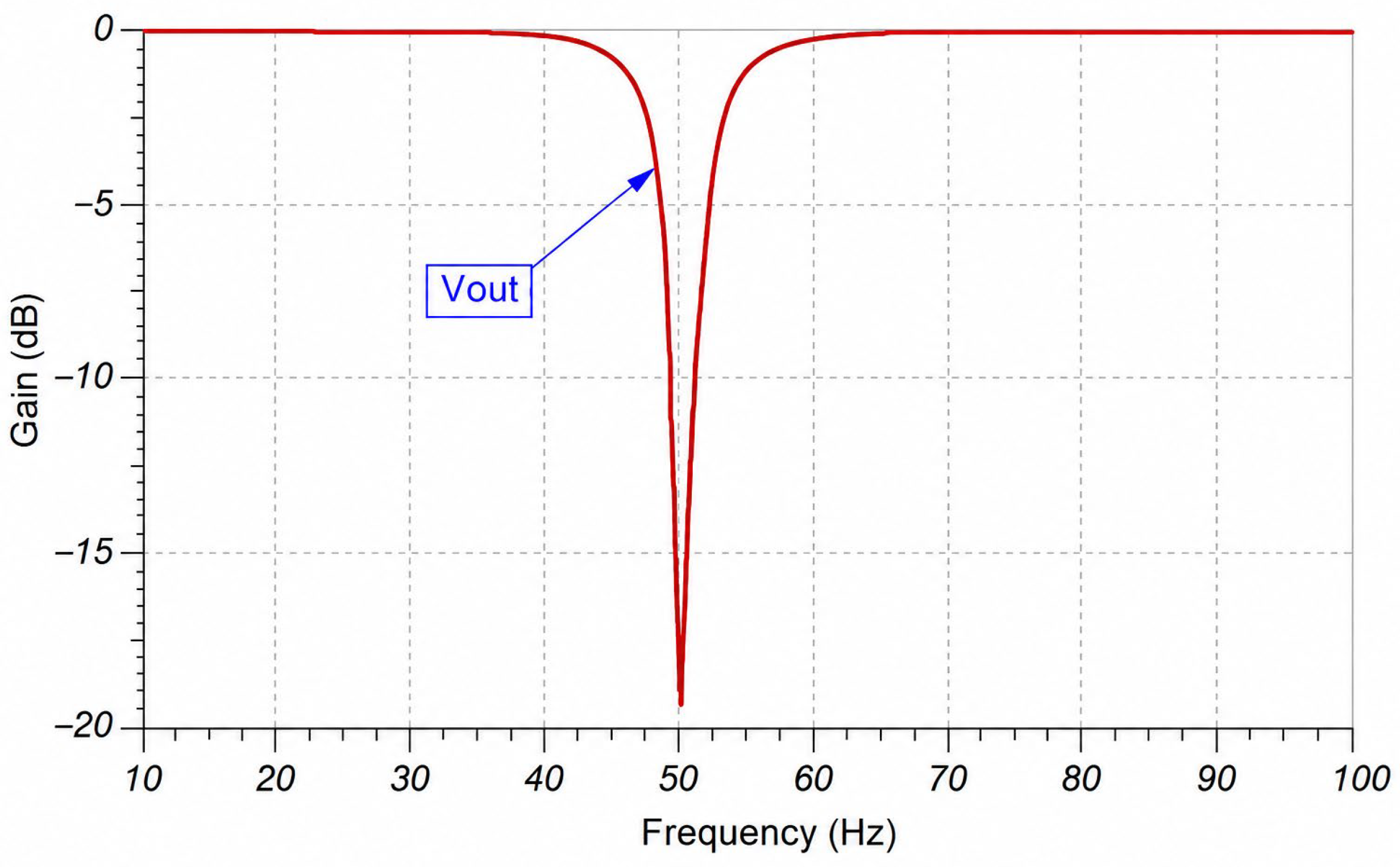
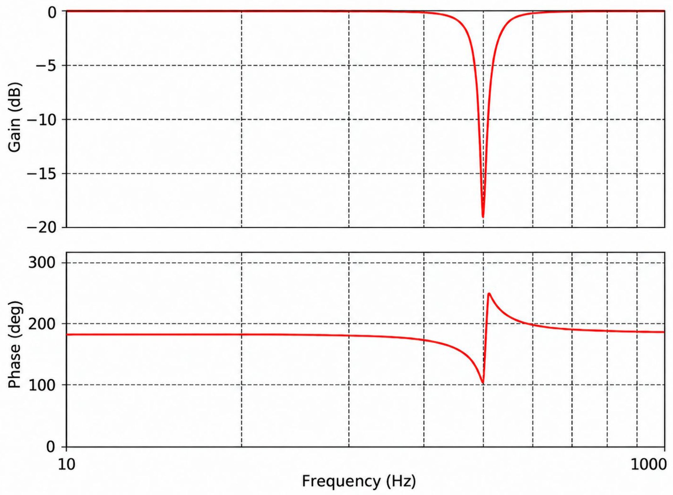
The frequency response of the voltage gain for the 50 Hz notch filter is shown in Figure 11.

The magnitude response of the filter is presented in Figure 11. A pronounced attenuation notch is observed around 50 Hz, confirming that the circuit effectively suppresses the 50 Hz mains-frequency component. Outside the rejection band, the attenuation remains low, allowing the desired signal components to pass with minimal distortion.

The TINA-TI simulation was also used to obtain the magnitude and phase responses of the 50 Hz notch filter, as shown in Figure 12.

Figure 12 presents the magnitude and phase characteristics of the 50 Hz notch filter. The phase response changes rapidly in the vicinity of the notch frequency, which is characteristic of narrow band-stop filters. Together, the magnitude and phase responses confirm the expected frequency-selective behavior of the analyzed circuit.

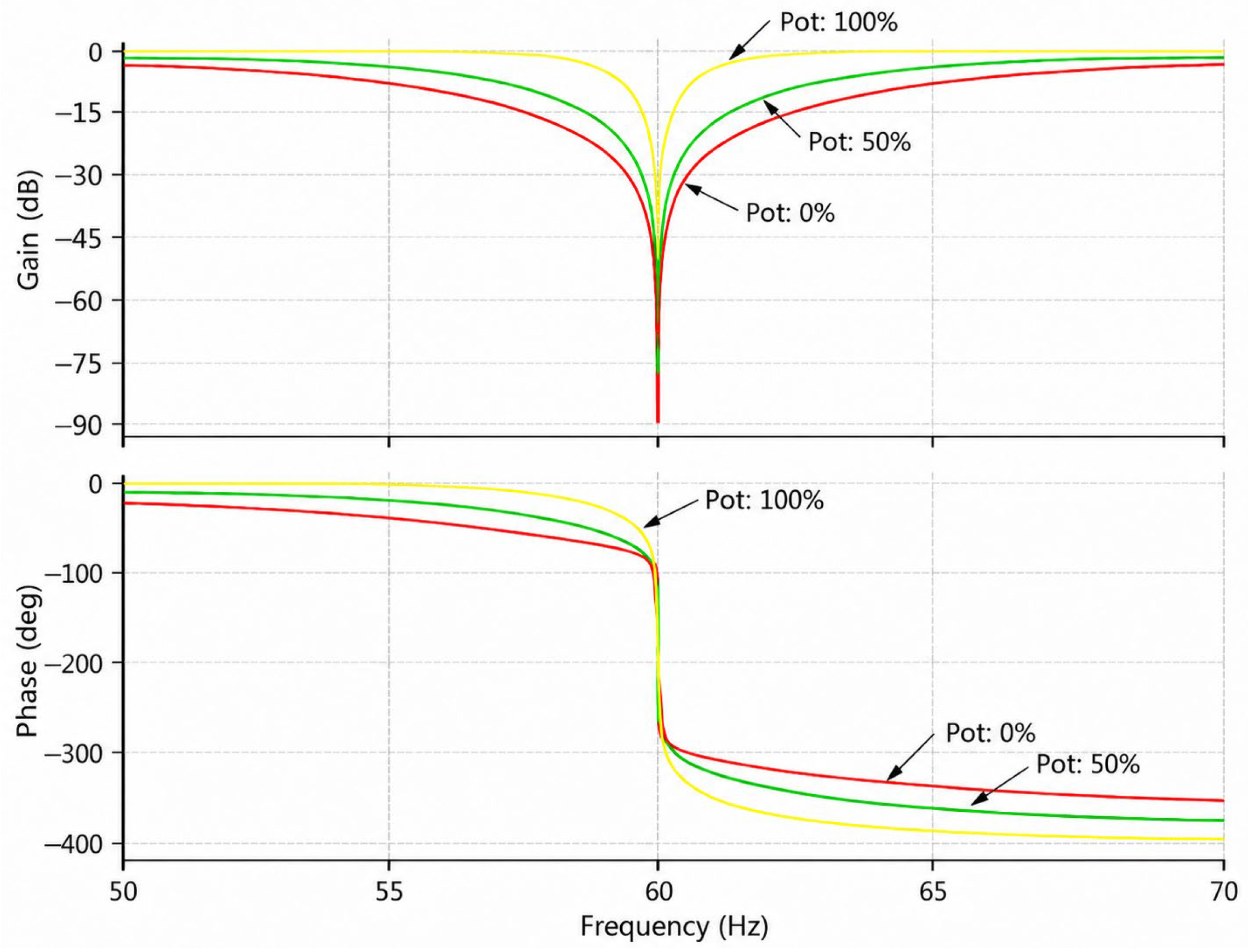
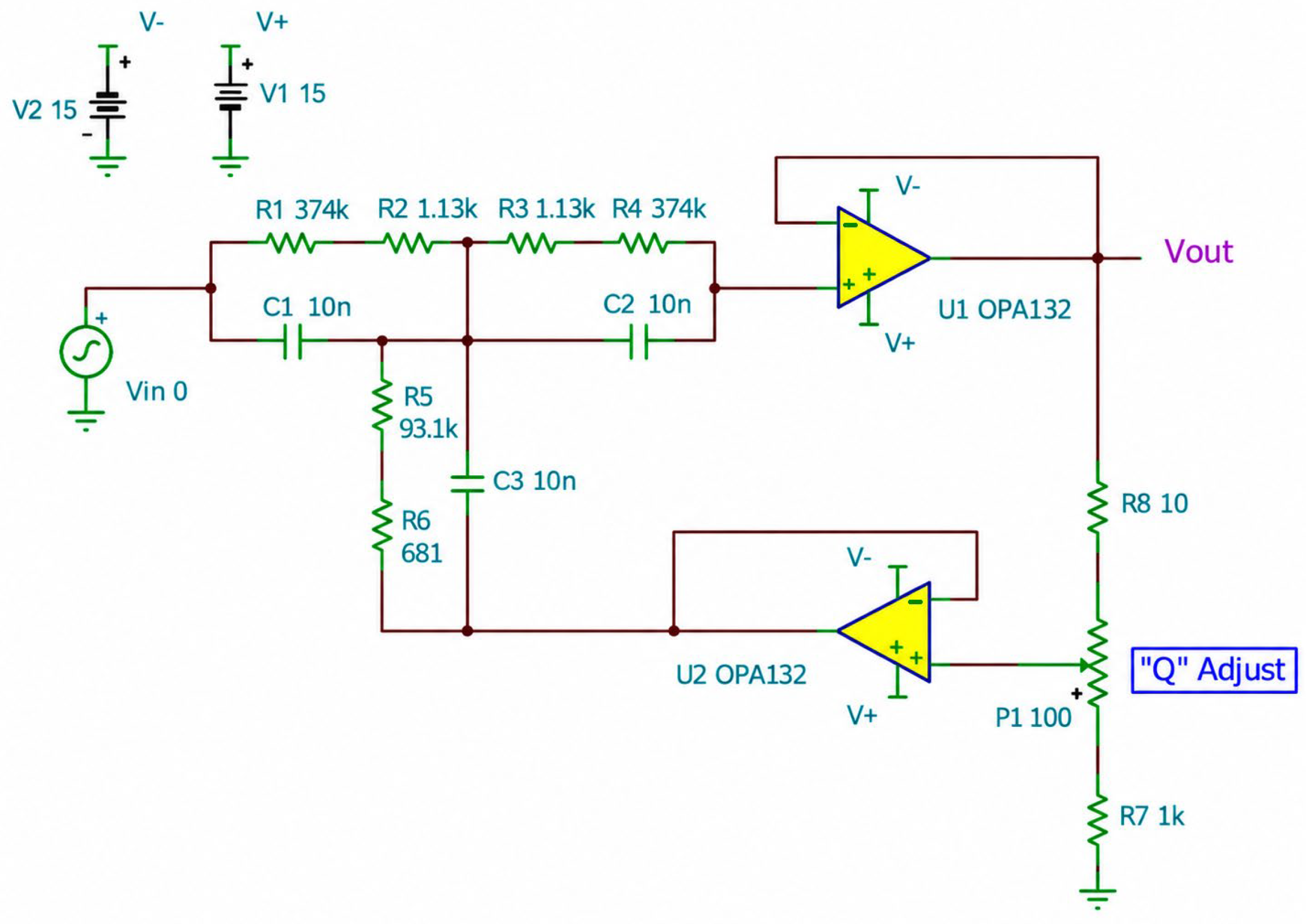
A second notch filter was analyzed for the suppression of 60 Hz power-line interference, corresponding to the mains frequency used in several countries. Unlike the 50 Hz UAF42-based implementation, the 60 Hz filter employs a discrete active-RC topology using OPA132 operational amplifiers. Although the two circuits have the same functional objective and are both second-order notch filters, they are based on different circuit implementations. Their comparison is therefore intended to illustrate two alternative realizations for mains-frequency interference suppression rather than a direct comparison of identical topologies shifted from 50 Hz to 60 Hz.

Figure 13 illustrates the schematic of the 60 Hz notch filter. Like the previous design, the filter selectivity is controlled through the quality factor, while accurate attenuation at the notch frequency requires precise component values and appropriate numerical convergence settings during simulation.

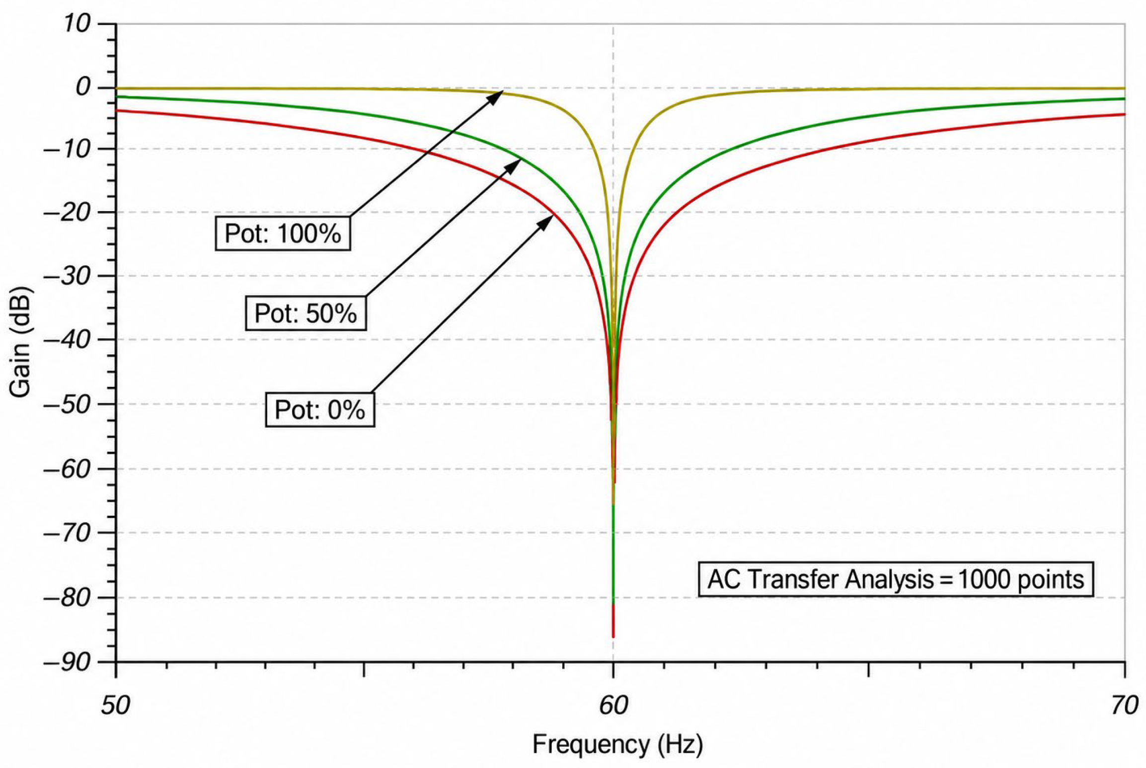
The magnitude response shown in Figure 14 confirms that the maximum attenuation occurs around 60 Hz. Apart from the narrow rejection band, the filter exhibits a nearly constant gain over the remaining frequency range, preserving the useful signal components.

Figure 15 presents the corresponding magnitude and phase characteristics of the 60 Hz notch filter. As expected, the attenuation minimum is located around 60 Hz, while the phase varies rapidly in the vicinity of the notch frequency. Although the frequency-domain behavior is similar to that of the 50 Hz filter, the two circuits employ different implementations.

The two notch filters considered in this section therefore represent alternative circuit realizations for power-line interference suppression. The 50 Hz design is based on the UAF42 universal active filter, whereas the 60 Hz design employs a discrete active-RC network with OPA132 operational amplifiers. Their comparison is intended to demonstrate that the same functional requirement—suppression of mains-frequency interference—can be achieved using different active-filter implementations.

Despite their different circuit realizations, both filters exhibit the expected narrow band-stop behavior around their respective target frequencies while maintaining a nearly constant response outside the rejection region.

2.4. Third-Order Butterworth High-Pass Filter

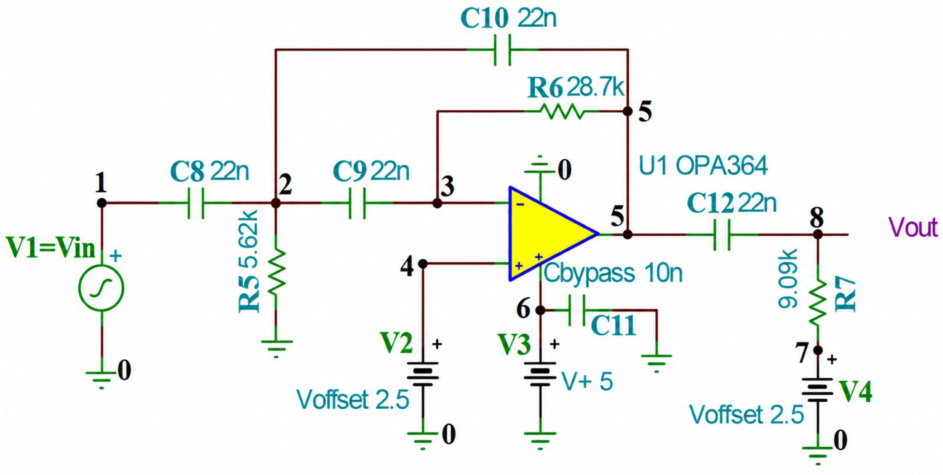
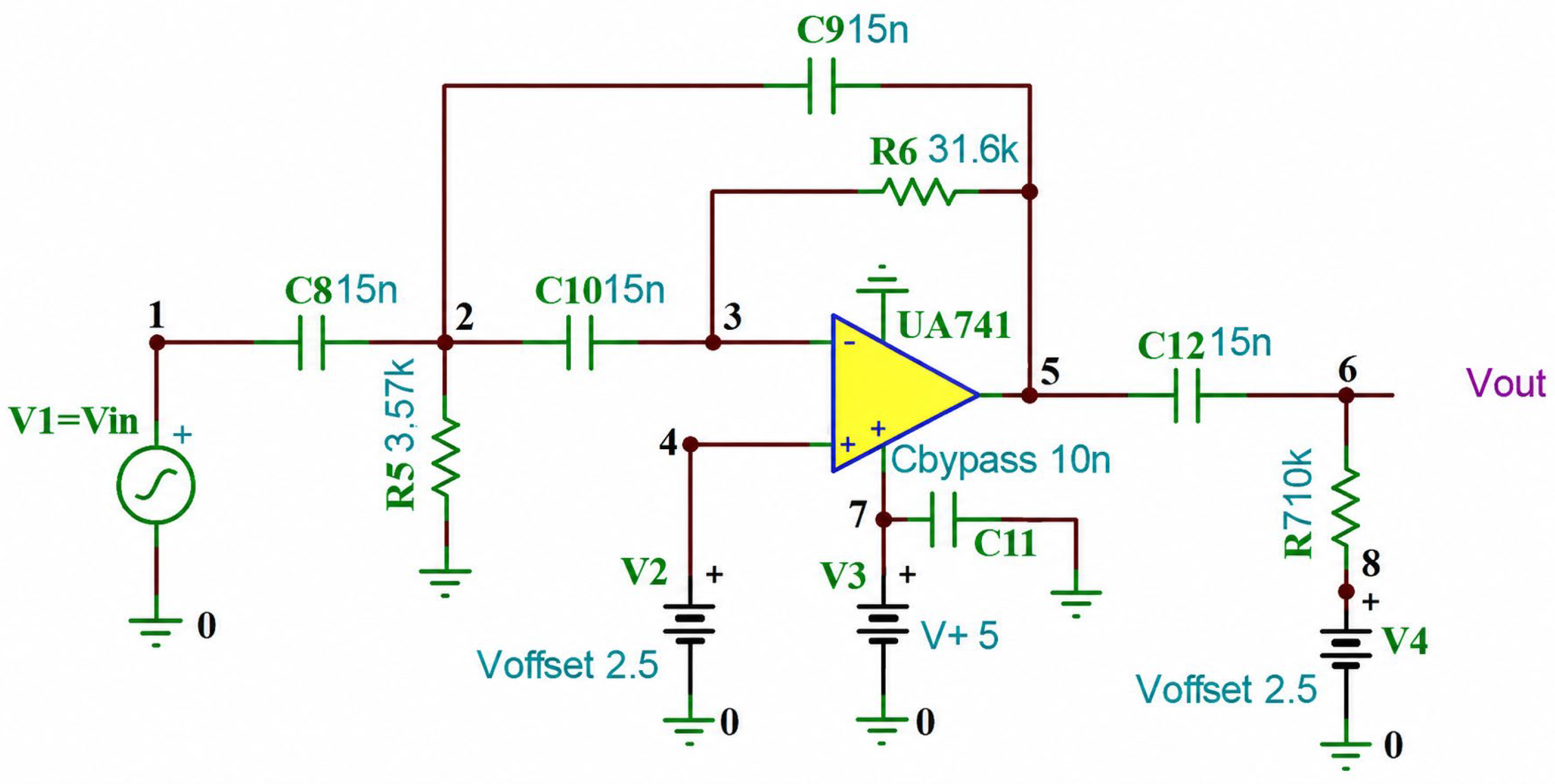
The third filter investigated in this study is a third-order Butterworth high-pass filter designed to provide a maximally flat magnitude response within the passband. Unlike the Bessel approximation, which emphasizes phase linearity and transient response, the Butterworth approximation is intended to achieve a smooth passband with no ripple while maintaining a steeper transition between the stopband and the passband. The circuit schematic used for the simulations is presented in Figure 16. Equivalent circuit implementations with the same nominal component values and target transfer characteristics were analyzed using SPICE, TINA-TI, MATLAB, MAPLE, ECAP, SYSEG, and TFSYG.

The circuit shown in Figure 16 implements a third-order active Butterworth high-pass filter. Like the previous examples, the operational amplifier was represented by an ideal voltage-controlled voltage source in the symbolic simulations, providing results directly comparable with those obtained using numerical circuit simulators. This approach enables a consistent evaluation of both numerical and symbolic analysis methods.

The SPICE and TFSYG input files used for the analysis are provided in Appendix A.3.

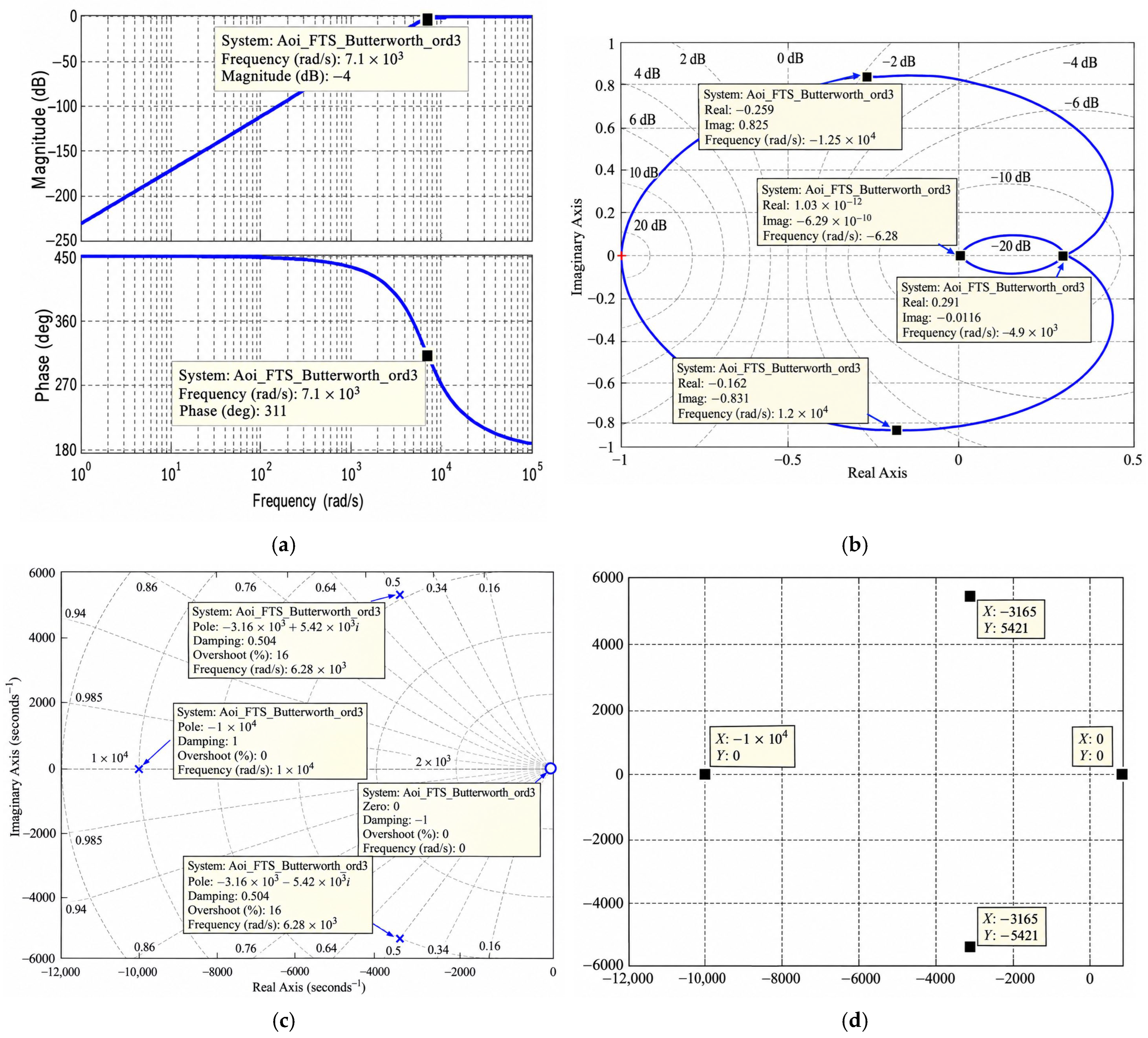
The frequency-domain characteristics of the Butterworth high-pass filter are presented in Figure 17. The Bode diagram exhibits the expected high-pass response, characterized by significant attenuation at low frequencies followed by a smooth transition toward a flat passband. As expected for the Butterworth approximation, no ripple is observed in the passband, while the attenuation slope increases with the filter order.

The Nyquist diagram confirms the stable behavior of the transfer function, and the pole-zero map indicates that all poles are in the left half of the complex plane. The symbolic pole-zero representation obtained using TFSYG is in close agreement with the numerical analysis, demonstrating the equivalence of the investigated simulation approaches.

For the symbolic analysis, the operational amplifier was replaced by an ideal voltage-controlled voltage source with a sufficiently high voltage gain. The resulting symbolic frequency response was found to be in close agreement with the numerical simulations.

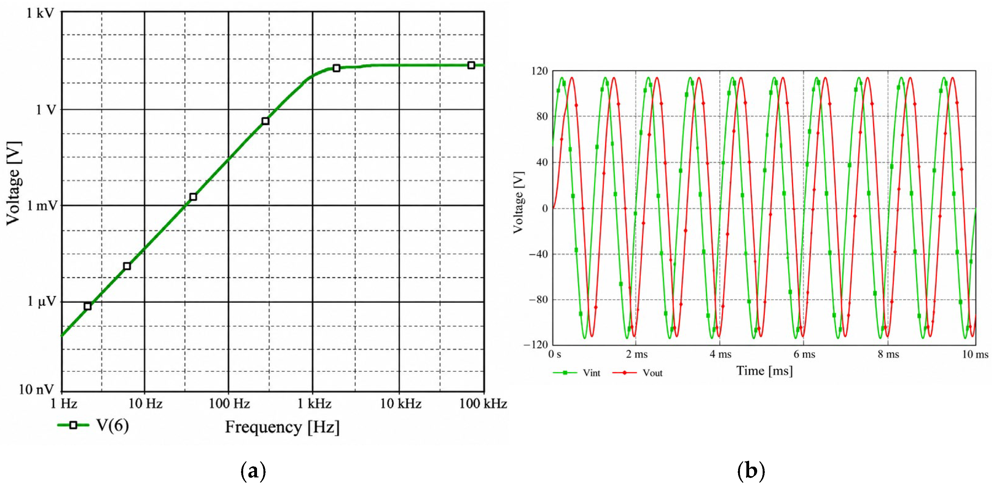
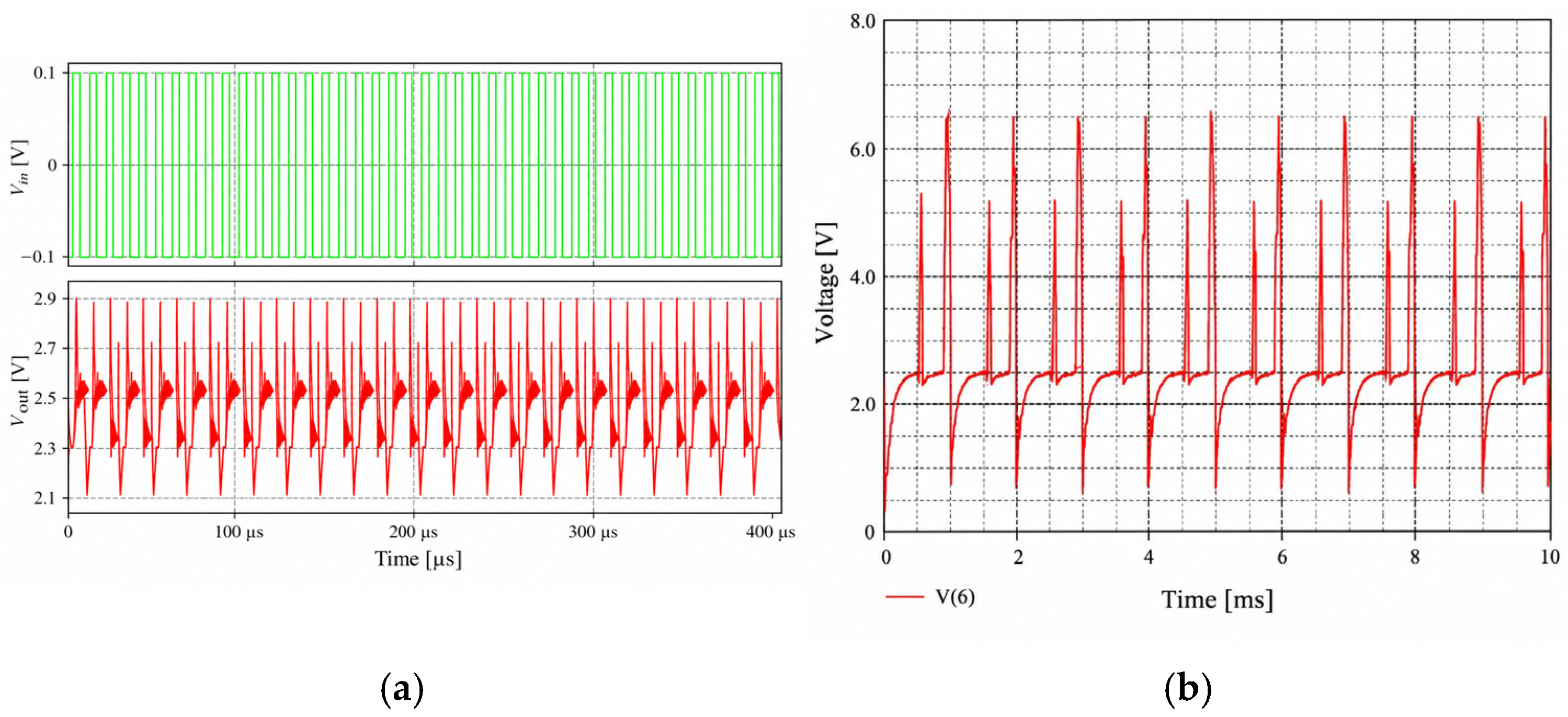
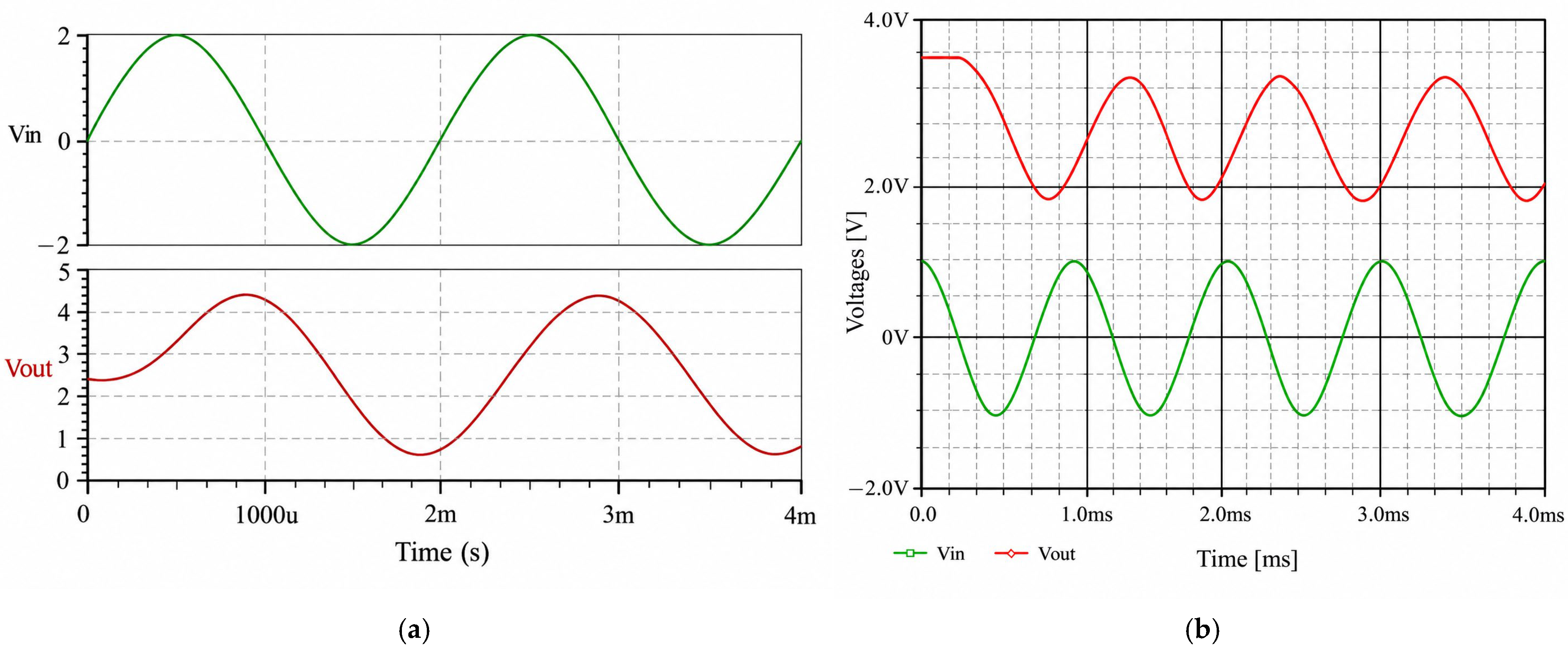
Figure 18 presents complementary numerical results for the third-order Butterworth high-pass filter. Panel (a) shows the magnitude response obtained using TINA-TI, while panel (b) shows the corresponding time-domain waveform obtained using SPICE. These results confirm the expected frequency-selective and transient behavior of the implemented filter model.

Figure 19 compares the transient responses obtained using the TINA-TI and SPICE simulation environments. The input and output voltage waveforms exhibit closely matching time-domain behavior, with only minor graphical differences resulting from the visualization formats adopted by each software package. The close agreement between the simulated waveforms further validates the analyzed Butterworth high-pass filter model.

The filter was designed using TI FilterPro Desktop v3.1(Texas Instruments, Dallas, TX, USA), which allows the cutoff frequency and voltage gain to be modified by updating the RC component values. The selected topology operates from a single supply and therefore requires DC offset voltage. When bipolar power supplies are available, this offset is no longer necessary. Furthermore, because low-frequency active filters frequently employ relatively large resistor values, operational amplifiers with CMOS or JFET input stages are generally preferred to minimize input bias currents and offset-voltage errors. If a non-inverting high-pass response is required, a Sallen–Key topology represents an appropriate alternative.

The frequency-domain and time-domain analyses presented in Figure 16, Figure 17, Figure 18 and Figure 19 show close agreement between the investigated software environments. The Butterworth high-pass filter exhibits the expected maximally flat passband together with stable transient behavior, while the numerical and symbolic analyses show close consistency. These findings confirm the reliability of the investigated software tools for the simulation, analysis, and verification of active Butterworth filter circuits.

2.5. Fifth-Order Sallen–Key Bessel Low-Pass Filter

Higher-order active filters can be implemented by cascading first- and second-order stages, with Sallen–Key structures providing a widely used realization for low-pass filter design [22]. In this study, a fifth-order Sallen–Key Bessel low-pass filter is considered as the final low-pass configuration. Compared with the third-order Bessel filter analyzed previously, its higher order provides improved attenuation of high-frequency components while preserving the favorable transient response and nearly linear phase characteristics associated with the Bessel approximation. The circuit schematic of the designed filter is presented in Figure 20. To ensure the reproducibility of the simulations, the corresponding SPICE and symbolic input files are included in Appendix A.4.

Figure 20 illustrates the fifth-order active Sallen–Key Bessel low-pass filter implemented using two operational-amplifier stages. Equivalent circuit implementations with the same nominal component values and target transfer characteristics were analyzed using SPICE, TINA-TI, CSAP, SYSEG, and TFSYG. As in the previous examples, equivalent numerical and symbolic models were employed to allow a direct comparison between the obtained simulation results.

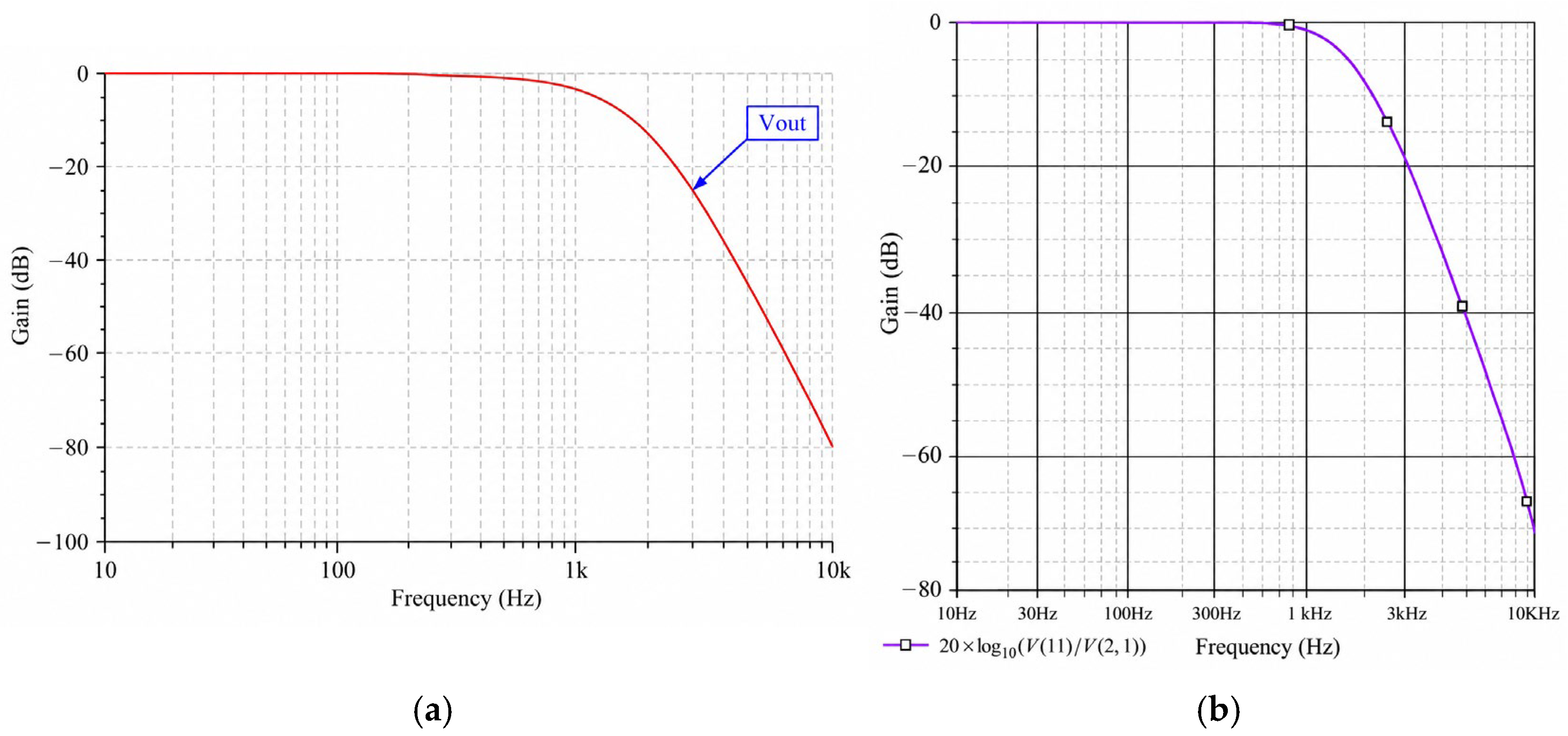
Figure 21 compares the magnitude responses obtained using the TINA-TI and SPICE simulation environments. Both responses exhibit the characteristic behavior of a fifth-order Bessel low-pass filter, maintaining an almost flat passband while providing a significantly steeper attenuation of high-frequency components compared with the third-order implementation. Although the graphical appearance differs because of the visualization tools available in each software package, the cutoff frequency and attenuation characteristics coincide over the entire analyzed frequency range, confirming the consistency of the numerical simulations.

Figure 22 compares the transient responses obtained using the TINA-TI and SPICE environments. The input and output voltage waveforms exhibit practically identical time-domain behavior, while only minor graphical differences arise from the visualization formats implemented by the two software packages. The preserved waveform shape confirms one of the principal advantages of the Bessel approximation, namely its superior transient response and reduced waveform distortion.

The frequency-domain and time-domain analyses demonstrate excellent agreement between the software environments investigated. The fifth-order Sallen–Key Bessel filter provides improved attenuation of high-frequency components compared with lower-order implementations while preserving the characteristic transient response of the Bessel approximation. The close agreement between the numerical and symbolic simulation results further confirms the reliability of the software tools investigated for the analysis and verification of high-order active filter circuits.

2.6. Band-Pass Filter Used in Voice Communications

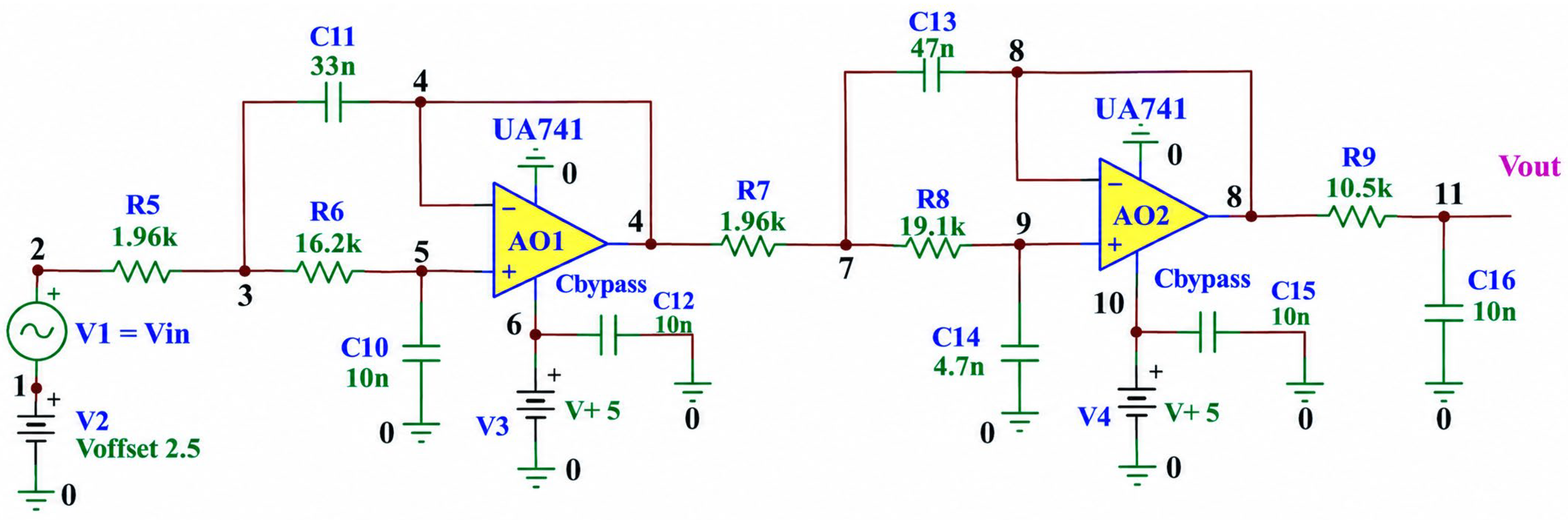
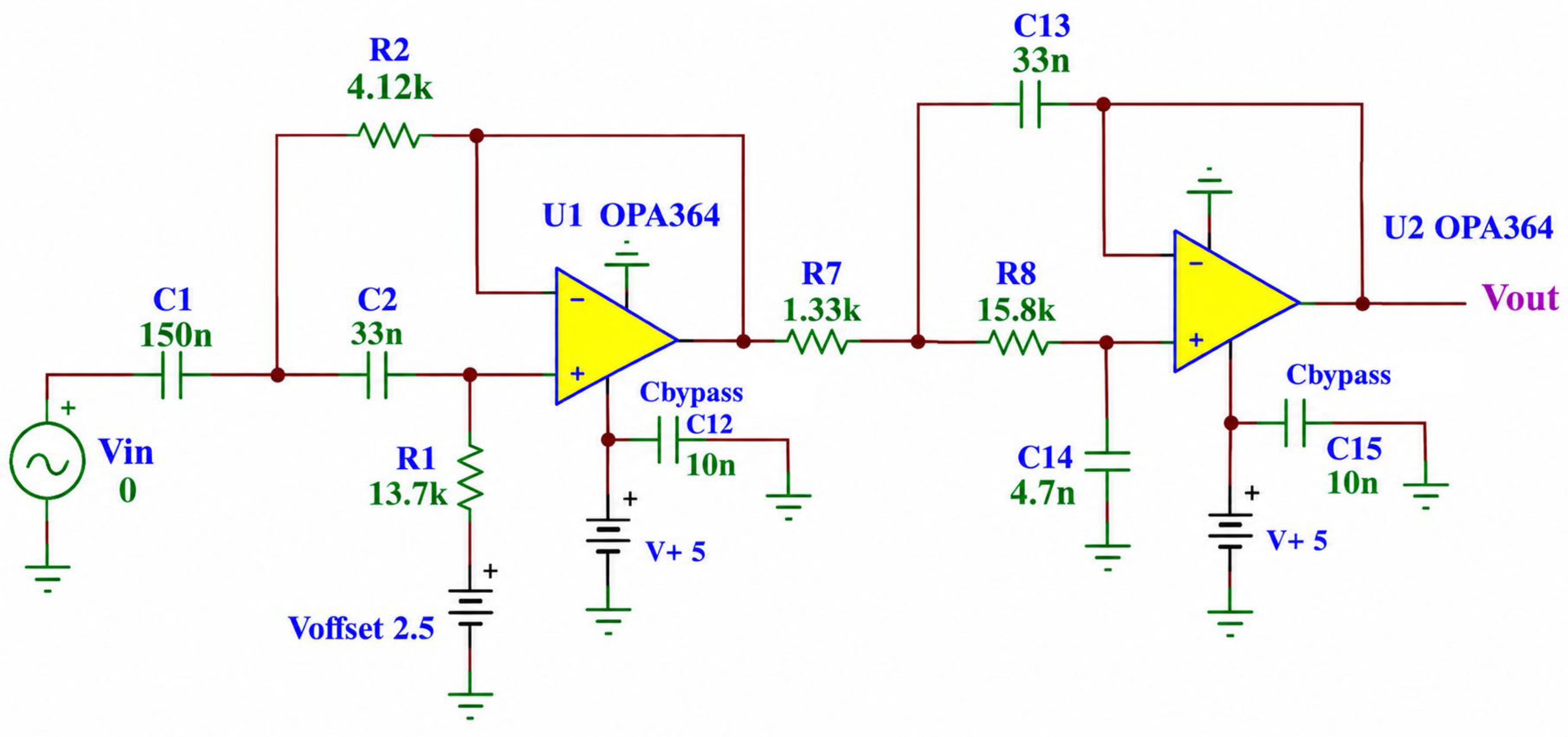
The final circuit investigated in this study is an active band-pass filter intended for voice-communication applications. The filter was designed to pass the useful speech-frequency components while attenuating both low-frequency disturbances and high-frequency noise. The selected passband extends approximately from 300 Hz to 2 kHz, corresponding to the frequency range required for conventional voice transmission systems. The circuit schematic is presented in Figure 23, while the corresponding symbolic input description is provided in Appendix A.5.

Figure 23 illustrates the active band-pass filter implemented using cascaded high-pass and low-pass Sallen–Key stages. Equivalent circuit implementations with the same nominal component values and target transfer characteristics were analyzed using SPICE, TINA-TI, CSAP, SYSEG, and TFSYG. As in the previous filter examples, equivalent numerical and symbolic models were employed to allow a direct comparison between the obtained simulation results.

$$AFTB\_FCom\_f={\displaystyle \frac{-(3871·{10}^{11}·f^2)}{(2130·{10}^5·f^4-9175·{10}^8·{\mathrm{I}·f}^3-8555·{10}^{11}·f^2+2521·{10}^{14}·\mathrm{I}·f+3512·{10}^{16}}}$$

(6)

The symbolic analysis provides the analytical expression of the voltage transfer function together with the corresponding poles and zeros. These quantities offer valuable information regarding the frequency selectivity and stability of the filter while enabling direct analytical verification of the numerical simulation results.

$$\begin{gathered} Poles\_AFTB\_FCom=\left[-1163+1121I,-4978,-\mathrm{19,730},-1163-1121,I\right] \\ \mathrm{Z}\mathrm{e}\mathrm{r}\mathrm{o}\mathrm{s}\_AFTB\_FCom=\left[0, 0\right] \end{gathered}$$

(7)

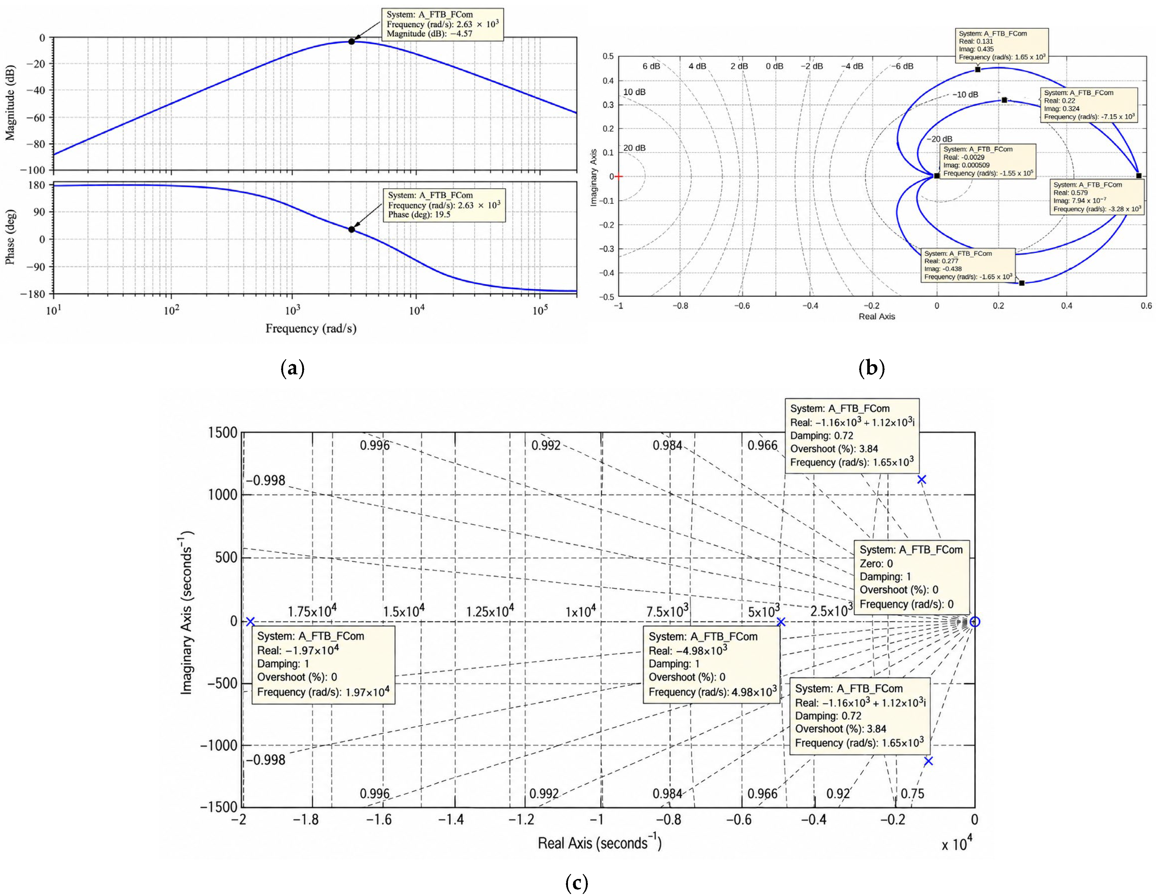
Figure 24 summarizes the frequency-domain characteristics of the proposed band-pass filter. The Bode diagram exhibits the expected band-pass response, characterized by strong attenuation below the lower cutoff frequency and above the upper cutoff frequency, while maintaining an almost constant gain within the useful voice band. The Nyquist diagram and the pole-zero map confirm the stability of the transfer function, as all poles remain located in the left half of the complex plane. The symbolic and numerical analyses show close agreement.

The filter was designed using TI FilterPro Desktop v3.1(Texas Instruments, Dallas, TX, USA), which allows the passband limits and voltage gain to be modified by recalculating the RC component values [23]. The proposed implementation employs cascaded Sallen–Key high-pass and low-pass stages operating from a single power supply; therefore, a DC offset voltage is required. When bipolar power supplies are available, this offset is unnecessary. Furthermore, operational amplifiers with CMOS or JFET input stages are generally preferred for low-frequency active filters to minimize offset-voltage errors associated with large resistor values.

The results presented in the previous subsections demonstrate that the investigated numerical and symbolic software environments provide highly consistent analyses when equivalent filter models and identical design parameters are employed. Although the graphical and analytical results show excellent agreement, the software tools investigated exhibit different capabilities depending on the type of analysis performed. To facilitate the overall interpretation of the obtained results,

Table 1. Comparative overview of the roles and analytical capabilities of the software environments investigated.

Software	Main Analysis Performed	Output Provided	Advantages Observed in This Study	Limitations Observed in This Study	Recommended Application
SPICE	Frequency response, transient analysis, AC/DC simulation	Numerical waveforms, Bode diagrams, transient responses	High numerical accuracy, realistic circuit simulation, reliable verification of filter behavior	Does not directly provide symbolic transfer functions or parameter sensitivities	Circuit validation and performance verification
TINA-TI	Frequency response, transient analysis, pole-zero analysis	Graphical responses, circuit measurements, pole-zero maps	User-friendly interface, rapid schematic implementation, integrated graphical analysis	Limited symbolic capabilities and analytical information	Educational use and rapid circuit development
MATLAB	Frequency-domain analysis, transient response, signal processing	Numerical plots, transfer-function evaluation, pole-zero maps	Flexible numerical computation, high-quality visualization, efficient post-processing of results	Symbolic capabilities require additional toolboxes and are less intuitive for circuit formulation	Numerical verification and data processing
MAPLE	Symbolic circuit analysis	Exact transfer functions, poles, zeros, symbolic expressions, sensitivities	Exact analytical solutions, parameter dependence, mathematical simplification	Less suitable for direct circuit simulation and transient analysis	Analytical derivation and theoretical validation
ECAP	Symbolic network analysis	Symbolic transfer functions and circuit equations	Efficient symbolic formulation of electrical networks with compact analytical expressions	Limited graphical visualization and numerical simulation features	Symbolic circuit modeling
SYSEG	Symbolic system analysis	State-space models, eigenvalues, symbolic matrices	Efficient system representation and analytical investigation of dynamic behavior	Intended primarily for analytical studies rather than practical circuit simulation	System-level analytical evaluation
TFSYG	Symbolic transfer-function generation	Exact transfer functions, poles, zeros	Fast derivation of transfer functions and analytical verification of filter models	Does not perform complete numerical simulation of circuit operation	Transfer-function derivation and symbolic verification

summarizes the principal characteristics, advantages, limitations, and recommended applications of each software environment.

Furthermore, the comparative assessment highlights that each software environment contributes distinct capabilities to the overall analysis process. While numerical simulation tools provide efficient evaluation of circuit behavior under practical operating conditions, symbolic software environments offer valuable analytical insight into circuit topology, transfer functions, and parameter dependencies. Consequently, selecting an appropriate software tool depends not only on the desired computational accuracy but also on the specific objectives of the analysis, whether focused on numerical verification, symbolic derivation, or comprehensive filter design.

The investigated software environments provide different output categories and therefore cannot be compared one-to-one for every performance indicator. SPICE and TINA-TI primarily provide circuit-level frequency- and time-domain responses, MATLAB supports independent numerical verification, while MAPLE, ECAP, SYSEG, and TFSYG provide complementary analytical or symbolic outputs, including transfer functions, circuit equations, state-space representations, and pole-zero information, according to their capabilities. The comparative framework therefore considers common, directly comparable quantities, while software-specific outputs provide complementary verification. Table 1 summarizes the roles, analytical capabilities, advantages, and limitations of each environment; these capabilities describe supported analyses and outputs rather than performance indicators quantitatively validated for every filter configuration.

To complement the qualitative comparison in Table 1 with a quantitative assessment of cross-platform agreement, three representative configurations were selected for detailed evaluation: the third-order Bessel low-pass filter, the third-order Bessel high-pass filter, and the third-order Butterworth high-pass filter. These cases were selected because corresponding numerical and symbolic results are available for the cutoff frequency, gain, phase, and pole locations. The quantitative indicators defined above were applied to the corresponding results, and the obtained values are summarized in

Table 2. Quantitative comparison of representative filter characteristics obtained from numerical and symbolic analysis.

Filter	Cutoff Frequency ${\mathit{f}}_{\mathit{c}}$ (Hz)	Gain at ${\mathit{f}}_{\mathit{c}}$ (dB)	Phase at ${\mathit{f}}_{\mathit{c}}$ (°)	Pole Locations (rad/s)	Gain Difference $\Delta \mathit{G}$ (dB)	Phase Difference $\Delta \mathit{\phi }$ (°)	Max. Pole-Location Deviation (%)
Third-order Bessel LPF	991.93	−3.0103	−99.20	$-8264.46;$ $-6579.22 \pm j6232.15$	0.0024	0.002	0.054
Third-order Bessel HPF	867.54	−3.0103	279.30	$-5000.50;$ $-2375.67 \pm j2664.17$	0.0046	0.097	0.460
Third-order Butterworth HPF	1266.41	−3.0103	296.09	$-\mathrm{10,000.00};$ $-3164.56 \pm j5420.56$	0.0026	0.145	0.073

Note: The cutoff frequency $f_c$ corresponds to the −3.0103 dB point relative to the passband level. For the third-order Bessel HPF, the value of 867.54 Hz represents the cutoff frequency determined according to this criterion, whereas 1 kHz denotes the nominal design frequency of the filter configuration. The maximum pole-location relative deviation was evaluated according to Equation (4). The third-order Bessel LPF has no finite zeros, whereas both high-pass filters have three coincident zeros at the origin (s = 0). Therefore, a relative zero-location deviation is not reported, since Equation (4) is undefined when the reference zero location is zero.

.

Table 2 confirms close numerical–symbolic agreement for the three representative filters, with gain differences below 0.005 dB, phase differences up to 0.145°, and a maximum pole-location deviation of 0.460%, while the other two cases remain below 0.1%. These results quantitatively support the agreement observed in the frequency-response and pole-zero plots.

The reported deviations apply to the adopted equivalent models and modeling assumptions. Larger differences may occur when non-ideal effects, including finite op-amp gain–bandwidth, slew-rate limitations, parasitic elements, component tolerances, or temperature dependence, are considered. The framework remains applicable provided that these effects are represented consistently in the compared models.

3. Conclusions

This paper presented a comprehensive comparative evaluation of representative active electrical filter structures using numerical simulation and symbolic-analysis software environments. The comparison was performed using equivalent circuit models, identical nominal component values, and common frequency-domain, time-domain, and symbolic analysis criteria, providing a consistent framework for evaluating the investigated software tools according to their respective capabilities.

The results demonstrated close agreement for the quantities that could be directly compared across the investigated numerical and symbolic software environments, including frequency responses, cutoff frequencies, pole-zero locations, transfer functions, and transient responses, according to the capabilities of each tool. The quantitative comparison performed for three representative filter configurations further confirmed that the deviations between corresponding numerical and symbolic results remained small under the adopted modeling assumptions. These findings support the consistency of the equivalent circuit models and common analysis criteria used in the present study.

The analyses further demonstrated that numerical simulation and symbolic analysis should be regarded as complementary rather than alternative approaches. Numerical software is particularly suitable for circuit-level frequency- and time-domain simulations and response verification, whereas symbolic software provides complementary analytical information, including transfer functions and pole-zero representations. Their combined use therefore provides a broader characterization of filter behavior by integrating numerical verification with analytical interpretation.

The principal contribution of this work is the establishment of a reproducible cross-platform framework for comparing numerical and symbolic software environments under equivalent modeling conditions. By maintaining equivalent filter models, identical nominal component values, and common evaluation criteria across the investigated tools, the methodology enables software-dependent differences to be distinguished more clearly from those associated with the underlying circuit model. Its application to several representative active-filter families demonstrates that the proposed procedure is not restricted to a single topology and may be extended to the comparative assessment of other analog circuits.