Article

Isoline Tracking Control of an Autonomous Underwater Helicopter in Unknown Marine Scalar Fields Under Noisy Measurements


1
School of Automation and Intelligent Science, Jiangnan University, Wuxi 214000, China
2
SINOPEC Research Institute of Petroleum Engineering Co., Ltd., Beijing 102206, China
*
Author to whom correspondence should be addressed.
Electronics 2026, 15(18), 4129; https://doi.org/10.3390/electronics15184129
Submission received: 7 August 2026 / Revised: 28 August 2026 / Accepted: 3 September 2026 / Published: 11 September 2026
(This article belongs to the Special Issue Robotics and Intelligent Control)

Abstract

For continuous boundary observation at a prescribed scalar level in unknown marine scalar fields, this paper proposes an isoline tracking method for an autonomous underwater helicopter (AUH) using only noisy local measurements. The method establishes an isoline kinematic relation based on the local scalar value and its rate of change. Without field reconstruction or compensation for unknown terms, it enables the AUH to stably approach the target isoline and maintain tangential motion, with adjustable tracking accuracy. To obtain reliable scalar-rate information from noisy measurements, a finite-time differentiator using current and historical noisy measurements was developed to suppress measurement noise while retaining the required dynamic response. A low-complexity prescribed-time velocity-matching controller was further developed in a direct algebraic form, allowing the contraction time and terminal range of the velocity errors to be specified without imposing restrictive conditions on finite initial errors. Simulation results in a suspended particulate matter scalar field and a temperature field verified the effectiveness of the proposed method.

1. Introduction

As marine resource development and underwater infrastructure continue to expand, underwater robots are being increasingly employed in underwater facility inspection, marine environmental monitoring, and deep-sea operations [1,2]. As a specialized autonomous underwater vehicle, the autonomous underwater helicopter (AUH) combines a compact disc-shaped configuration with hovering capability and flexible multidirectional maneuverability, making it well suited to low-speed observation tasks near the seabed or underwater structures that require frequent heading and velocity adjustments [3,4]. Marine scalar fields arise in applications such as suspended particulate plume observation, pollutant dispersion monitoring, and thermal anomaly detection. Continuous tracking of a prescribed scalar level provides boundary information for characterizing the extent and spatial evolution of an affected region under specific environmental conditions [5,6,7].
In unknown marine scalar fields, underwater vehicles generally have access only to local scalar measurements, while the global field distribution and the geometry of the target isoline remain unavailable and may vary with environmental conditions. Consequently, the vehicle cannot directly determine its position relative to the target isoline or the local tangential direction required for continuous boundary following. To address this problem, related studies have investigated marine environmental feature tracking from different perspectives. Tian et al. [8] integrated front reconstruction, Bayesian optimization, and nonlinear model predictive control to generate and track a smooth reference path along an ocean front. Mo-Bjørkelund et al. [9] employed an onboard boundless Gaussian random field model to adaptively explore a dynamic river plume boundary. Zhang and Li [10] combined an advection–diffusion model with a PDE observer to estimate and track the dynamic boundary of a suspended sediment plume. Von See et al. [11] used a UKF-based gradient estimator and extremum-seeking control to detect and follow ocean layers from in situ temperature measurements. Song et al. [12] developed a gradient-free isoline tracking law based on local sensing information and its variation rate, thereby reducing the dependence on global position information. These studies provide an important basis for marine environmental feature tracking. However, field-reconstruction and model-based methods require environmental models or online field estimation, whereas gradient-based methods rely on gradient estimation or additional excitation. Gradient-free methods reduce these information requirements but generally require the temporal variation rate of the local measurement, which cannot be obtained directly from a scalar sensor and is susceptible to noise amplification during numerical differentiation.
To obtain reliable rate information from noisy measurements, extensive studies have investigated differentiator and filtering designs. Calmbach et al. [13] optimized the gain scaling of homogeneous differentiators to reduce the influence of measurement noise on differentiation errors. Aldana-López et al. [14] developed a robust exact first-order differentiator with Lipschitz-continuous output and optimal worst-case accuracy. Seeber [15] proposed an implicit discrete implementation of robust exact differentiators with noise-filtering capability for sampled measurements. Lin et al. [16] combined a super-twisting differentiator with an event-triggered extended state observer to improve noise attenuation and disturbance estimation. Guo et al. [17] introduced a tracking differentiator with phase compensation to suppress measurement noise while reducing the response delay caused by low-pass filtering. These studies have improved differentiation accuracy, output smoothness, and digital implementation under noisy measurements. Nevertheless, for isoline tracking based on local scalar measurements, the scalar-rate estimate must suppress measurement noise while preserving the dynamic variation required for real-time yaw regulation.
Prescribed-performance and prescribed-time control have also been extensively investigated to regulate the transient and steady-state behavior of marine vehicles. Liu et al. [18] combined a predefined-time disturbance observer with terminal sliding-mode control for AUV trajectory tracking. Sui et al. [19] integrated a prescribed-time extended-state observer, prescribed-performance constraints, and dynamic-surface control for USVs. Chen et al. [20] developed an adaptive disturbance-observer-based fixed-time sliding-mode controller with prescribed performance. Fan et al. [21] introduced an actor–critic reinforcement-learning framework and an auxiliary compensation system into predefined-time USV control. Xia et al. [22] addressed initial-feasibility and singularity problems through parameterized nonmonotonic performance constraints.
Taken together, three issues remain particularly relevant to AUH isoline tracking in unknown marine scalar fields: dependence on prior field information, reliable acquisition of the scalar rate under measurement noise, and the implementation complexity of prescribed-performance control. To address these issues, this paper develops an AUH isoline-tracking framework using noisy local scalar measurements. The main contributions are summarized as follows.
  • Unlike marine feature tracking methods based on environmental mapping, contour prediction, or planned survey paths [23,24,25], the proposed method establishes an isoline kinematic relation in an unknown marine scalar field using the local scalar value and its rate of change at the current position of the AUH. Without obtaining or exactly compensating for the unknown time-varying Hessian coupling term, the AUH can approach the target isoline and maintain stable tangential motion.
  • Unlike direct finite-difference estimation and conventional low-pass filtering [26], an online scalar-rate estimation scheme was developed for noisy local scalar measurements. The differentiator exactly recovers the scalar rate within a finite time in the absence of noise and provides an explicit estimation error bound under bounded noise.
  • Unlike prescribed-performance underwater-vehicle controllers that combine neural networks, state or disturbance observers, or event-triggered compensation mechanisms [27,28,29], a low-complexity prescribed-time velocity-matching controller was designed. The controller prescribes the error contraction time and terminal range without restricting the magnitude of finite initial velocity errors and guarantees stable tracking of the desired velocity after the prescribed time through a direct algebraic control law.
The remainder of this paper is organized as follows. Section 2 presents the AUH model, isoline kinematics, and control objectives. Section 3 develops the virtual yaw control, scalar-rate estimator, and prescribed-time velocity-matching controller, together with the stability analysis. Section 4 presents the simulation validation in two marine scalar fields, comparative analysis, and a prospective experimental validation scheme. Section 5 concludes the paper.

2. Preliminaries and Problem Description

This section presents the horizontal-plane motion model of the AUH, the isoline kinematic description in an unknown marine scalar field, and the control objectives.

2.1. Horizontal-Plane Motion Model of the AUH

Consider the three-degree-of-freedom motion of the AUH in the horizontal plane. Its horizontal-plane kinematic and dynamic model is expressed as
η ˙ h = J ( ψ ) v h , M v ˙ h + F h ( v h ) = τ t h + d + Δ ,
where η h = col ( r , ψ ) denotes the horizontal-plane pose vector of the AUH, r = col ( x , y ) denotes its position in the inertial coordinate frame, and ψ denotes the heading angle; v h = col ( u , v , ω ) denotes the velocity vector in the body-fixed coordinate frame, where u, v, and ω are the surge velocity, sway velocity, and yaw angular velocity, respectively. Furthermore, the cruising speed of the AUH is expressed as v c = u 2 + v 2 . The matrix M denotes the inertia matrix; F h ( v h ) denotes the nonlinear hydrodynamic terms including the Coriolis, centripetal, and damping terms; d and Δ denote the environmental disturbance and the model uncertainty caused by unmodeled hydrodynamics and parameter perturbations, respectively; and τ t h denotes the control forces and moment acting on the AUH.
The coordinate transformation matrix J ( ψ ) is given by
J ( ψ ) = cos ψ sin ψ 0 sin ψ cos ψ 0 0 0 1 .
The relationship between the control forces and the thruster control input is expressed as
τ t h = G 0 τ u .
Here, G 0 denotes the thrust allocation matrix, and τ u = col ( τ u , 1 , τ u , 2 , τ u , 3 ) denotes the thruster control input vector, where τ u , 1 , τ u , 2 , and τ u , 3 are the control inputs of the three thrusters, respectively.
A three-thruster horizontal-plane configuration is adopted in this study. Thrusters 1 and 2 are symmetrically arranged along the longitudinal direction of the AUH. Together, they generate the surge force, while their thrust difference generates the yaw moment. Thruster 3 is arranged along the transverse direction of the AUH to generate the sway force. The corresponding thrust allocation matrix is selected as
G 0 = 1 1 0 0 0 1 1 1 0 .
Assumption 1.
The environmental disturbance d and the model uncertainty Δ are bounded unknown terms.
Define the transformed velocity as L = J ( ψ ) v h . Combining Equations (1) and (2), the system model can be further expressed as
η ˙ h = L , L ˙ = J ˙ ( ψ ) v h + J ( ψ ) M 1 ( d + Δ ) J ( ψ ) M 1 F h ( v h ) + J ( ψ ) M 1 G 0 τ u .
To construct a hierarchical control structure that does not rely on continuous global position feedback, the system is decomposed into the parts associated with the horizontal position and heading. Define the transformed state variable
ϑ = q x q y = cos ψ sin ψ sin ψ cos ψ u v ,
where q x = x ˙ and q y = y ˙ denote the horizontal velocity components of the AUH along the x- and y-axes of the inertial coordinate frame, respectively.
Furthermore, it follows that L = col ( ϑ , ω ) , and the system can be decomposed as
r ˙ = ϑ , ϑ ˙ = a + τ a , ψ ˙ = ω , ω ˙ = b + τ b ,
where = col ( a , b ) = J ˙ ( ψ ) v h + J ( ψ ) M 1 ( d + Δ ) J ( ψ ) M 1 F h ( v h ) and τ = col ( τ a , τ b ) = J ( ψ ) M 1 G 0 τ u . The superscripts a and b denote the variables associated with the horizontal-position subsystem and the heading subsystem, respectively.
The two subsystems are coupled through the heading angle ψ and the corresponding yaw motion. The yaw angular velocity ω changes the heading angle ψ, thereby adjusting the direction of motion of the AUH and subsequently affecting the evolution of the horizontal position r.

2.2. Isoline Kinematic Description in an Unknown Marine Scalar Field

Consider an unknown marine scalar field F : Ω R + defined over a two-dimensional domain Ω R 2 . Let r ( t ) denote the position of the AUH at time t. The true scalar value at its current position is expressed as
s ( t ) = F ( r ( t ) ) .
For a given target scalar value s d , the corresponding target isoline set is defined as
C ( s d ) = r Ω | F ( r ) = s d .
Unknown marine scalar fields commonly arise in tasks such as marine leakage monitoring, pollutant dispersion observation, and thermal anomaly detection. In such scenarios, leakage sources, pollution sources, thermal sources, or other anomalous regions can be regarded as a field-source region S , around which a spatially continuous scalar-field distribution is formed. Different scalar values correspond to different isolines, and C ( s d ) denotes the target isoline associated with the scalar value s d . Cruising along this isoline enables the AUH to continuously observe spatial regions with the same scalar level, thereby providing continuous boundary information for identifying the extent of the affected region and evaluating its spatial evolution.
The position of the source region, the global distribution of the scalar field, and the geometric shape of the target isoline are all unknown. To illustrate the spatial distribution of the scalar field and the isoline-tracking process of the AUH, the analytical scenario shown in Figure 1 is introduced. In the typical scalar-field scenario shown in Figure 1, the positive scalar-gradient direction points from the current position toward the region in which the local scalar value increases. The variable β denotes the directed angle from the x-axis of the inertial coordinate frame to the positive scalar-gradient direction at the current position, while ϕ denotes the directed angle from the heading direction of the AUH to the positive scalar-gradient direction. By regulating the geometric relationship between its heading and the local scalar-gradient direction, the AUH approaches the target isoline and cruises along it.
According to the geometric relationship shown in Figure 1, the following angular relationship is obtained:
ϕ = β ψ .
Let g ( r ) denote the magnitude of the scalar-field gradient at the current position r. Then,
g ( r ) = F ( r ) , F ( r ) = g ( r ) cos β sin β .
In the isoline kinematic analysis, the AUH moves at the fixed cruising speed v d along the heading angle ψ . Its position dynamics are expressed as
r ˙ ( t ) = v d h ( ψ ) , h ( ψ ) = cos ψ sin ψ ,
where h ( ψ ) is the unit direction vector corresponding to the heading of the AUH.
Assumption 2.
There exists an unknown high-concentration source region S within the operating region of the AUH. The target isoline C ( s d ) is a smooth closed curve enclosing this region, and the concentration near the high-concentration source region is higher than that in the surrounding area. The unknown concentration field F ( r ) is twice continuously differentiable in Ω, and within the operating region relevant to the target-isoline tracking task, there exist positive constants γ 1 , γ 2 , and γ 3 such that
0 < γ 1 F ( r ) γ 2 , 2 F ( r ) γ 3 , r Ω .
The lower-bound condition therefore does not require the scalar-field gradient to remain uniformly nonzero over the entire physical field. When the AUH approaches a locally weak-gradient region, the available decay margin in the scalar-tracking dynamics decreases, while the bounds associated with the directed-angle variation become more conservative. Consequently, the predicted ultimate bounds on the scalar-tracking error and directed angle may increase. If the actual gradient temporarily falls below the adopted lower bound γ 1 , the sufficient conditions in Lemma 1 and Theorem 1 are no longer guaranteed over that interval, but this does not imply loss of controller operation. Once the AUH returns to a region satisfying the gradient condition, the stated theoretical guarantees apply again.
It should be noted that γ 1 , γ 2 , and γ 3 are envelope constants used for the sufficient stability conditions and gain selection, rather than online field information required by the controller. In practice, they can be conservatively estimated over the relevant target-isoline operating region using available historical survey data, calibration data, or preliminary local measurements, without requiring reconstruction of the global scalar field.
Taking the time derivative of the scalar value along the motion trajectory of the AUH and combining Equations (9) and (10), the chain rule gives
s ˙ = F ( r ) T r ˙ = v d g ( r ) cos β cos ψ + sin β sin ψ = v d g ( r ) cos ( β ψ ) = v d g ( r ) cos ϕ .
To specify the desired tangential cruising direction of the AUH, the desired directed angle is selected as ϕ d = π / 2 . When ϕ = ϕ d , the heading of the AUH is orthogonal to the scalar-gradient direction. It follows from Equation (12) that s ˙ = 0 , and the AUH moves along the tangential direction of the concentration isoline passing through its current position. Since s ˙ = 0 only indicates that the concentration at the current position remains unchanged, the ideal state of target-isoline tracking should simultaneously satisfy s = s d and ϕ = π / 2 .

2.3. Control Objectives

The control objectives of this study are divided into the following two levels.
1. Isoline tracking: The AUH is required to approach and remain within a neighborhood of the target isoline C ( s d ) while cruising along its tangential direction, that is,
lim sup t | s ( t ) s d | ε s , lim sup t ϕ ( t ) π 2 ε a .
where ε s > 0 and ε a > 0 are the adjustable neighborhood bounds for the scalar-tracking error and the tangential-angle error, respectively.
2. Velocity matching: The cruising speed and yaw angular velocity of the AUH are required to enter and remain within prescribed terminal neighborhoods of their desired values v d and ω d by the prescribed time T c , respectively, that is,
| v c ( t ) v d | < ε v , | ω ( t ) ω d ( t ) | < ε ω , t T c .
where ε v > 0 and ε ω > 0 are the prescribed terminal bounds for the cruising-speed and yaw-rate errors, respectively.

3. Control Design

This section first describes the design of the virtual yaw angular velocity based on the scalar-tracking error and its rate of change. A scalar-rate estimation method is then developed for noisy concentration measurements, followed by the construction of a low-complexity velocity-matching controller.

3.1. Virtual Yaw Angular Velocity Design

In the ideal isoline motion state, the AUH should satisfy s = s d and ϕ = π / 2 . According to Equation (12), one has s ˙ = 0 . To continuously maintain the same scalar value along the motion trajectory of the AUH, it is also necessary to satisfy s ¨ = 0 .
First, differentiating Equation (12) and applying the product rule give
s ¨ = d d t F ( r ) T r ˙ + F ( r ) T r ¨ .
Next, applying the chain rule and using the symmetry of 2 F ( r ) , together with Equations (9) and (10), yield
s ¨ = v d g ( r ) sin ϕ ω + v d 2 h T ( ψ ) 2 F ( r ) h ( ψ ) .
The first term represents the effect of the yaw motion of the AUH on the scalar-value rate, whereas the second term is the field coupling term induced by the spatial variation of the scalar-field gradient as the AUH moves along its current heading.
When sin ϕ 0 , the instantaneous yaw angular velocity required to continuously maintain s ˙ = 0 in the ideal isoline motion state is
ω * ( t ) = v d h T ( ψ ) 2 F ( r ) h ( ψ ) g ( r ) sin ϕ .
In particular, at the desired tangential state ϕ = π / 2 , one has
ω * ( t ) = v d h T ( ψ ) 2 F ( r ) h ( ψ ) g ( r ) .
Equation (17) shows that the yaw angular velocity required to exactly maintain isoline motion depends on the local scalar-gradient magnitude and the Hessian matrix. For a general unknown marine scalar field, this field information is unknown and varies with the position of the AUH. Consequently, the ideal yaw angular velocity has an unknown position-dependent characteristic, and a yaw angular velocity applicable to the entire motion process cannot be specified before the task to continuously maintain the isoline motion of the AUH.
Therefore, instead of directly estimating or compensating for the unknown field coupling term, the virtual yaw angular velocity is constructed using the local scalar value and its rate of change at the current position. Define the scalar-tracking error as e s ( t ) = s ( t ) s d . Since s d is constant, one has e ˙ s ( t ) = s ˙ ( t ) . The composite error is further defined as
e p ( t ) = e ˙ s ( t ) + k 2 tanh e s ( t ) k 3 ,
where k 2 > 0 is the scalar-error regulation gain, and k 3 > 0 is the scaling parameter of the hyperbolic tangent function.
When e p ( t ) = 0 , the scalar-tracking error satisfies
e ˙ s ( t ) = k 2 tanh e s ( t ) k 3 .
Therefore, as the composite error approaches zero, the concentration error approaches zero under the hyperbolic tangent feedback. The hyperbolic tangent term limits the regulation magnitude when the scalar-tracking error is large and retains a locally linear regulation characteristic near the target isoline.
Based on the composite error in Equation (18), the virtual yaw angular velocity is designed as
ω d ( t ) = k 1 e p ( t ) ,
where k 1 > 0 is the virtual yaw control gain.
To distinguish the virtual yaw angular velocity from the actual yaw motion, define the yaw-rate matching error as e v , 3 ( t ) = ω ( t ) ω d ( t ) . Hence, ω = ω d + e v , 3 .
Using this relation together with Equation (19), Equation (16) becomes
s ¨ = k 1 v d g ( r ) sin ϕ e p + v d g ( r ) sin ϕ e v , 3 + v d 2 h T ( ψ ) 2 F ( r ) h ( ψ ) .
Differentiating the composite error in Equation (18) and using Equation (20) give
e ˙ p = k 1 v d g ( r ) sin ϕ e p + v d g ( r ) sin ϕ e v , 3 + v d 2 h T ( ψ ) 2 F ( r ) h ( ψ ) + k 2 k 3 sech 2 e s k 3 e ˙ s .
The term v d g ( r ) sin ϕ e v , 3 explicitly represents the influence of the velocity-matching dynamics on the scalar-tracking subsystem and vanishes under exact yaw-rate matching.
For practical gain selection, the prescribed-performance parameters κ and introduced in Section 3.3 can first be selected according to the desired terminal velocity-matching accuracy, and the terminal component-wise velocity-matching bound is defined as e ¯ v κ / 1 2 . According to Theorem 3 and Equation (50), | e v , 3 ( t ) | < e ¯ v for all t T c . Therefore, e ¯ v can be calculated explicitly before selecting k 1 and does not require an a priori bound on e v , 3 during the velocity-matching contraction interval t 0 t < T c . Accordingly, the following scalar-tracking stability analysis is stated from T c onward.
Whether the feedback term k 1 v d g ( r ) sin ϕ e p in Equation (21) suppresses the composite error depends on the sign of sin ϕ . To maintain the feedback polarity and ensure a uniform positive lower bound for the decay coefficient, the directed angle must remain in a region where sin ϕ > 0 .
Accordingly, define the angular region
D ϕ = ε ϕ , π ε ϕ , 0 < ε ϕ < π 2 .
For any ϕ D ϕ , one has sin ϕ sin ε ϕ > 0 . If this region is positively invariant, the decay coefficient in the composite-error dynamics satisfies
k 1 v d g ( r ) sin ϕ k 1 v d γ 1 sin ε ϕ > 0 .
To analyze the positive invariance of D ϕ , define the unit tangent vector of the scalar-gradient direction as τ g = [ sin β , cos β ] T . From the variation of the gradient vector along the motion trajectory of the AUH, one obtains
β ˙ = τ g T 2 F ( r ) r ˙ F ( r ) .
According to Assumption 2 and Equation (10),
β ˙ v d γ 3 γ 1 .
Lemma 1.
Suppose that the directed angle at the prescribed time satisfies ϕ ( T c ) D ϕ , and the control parameters satisfy
0 < k 2 < v d γ 1 cos ε ϕ , k 1 > v d γ 3 / γ 1 + e ¯ v v d γ 1 cos ε ϕ k 2 .
Then, D ϕ is a positively invariant set; that is, ϕ ( t ) D ϕ for all t T c .
The proof is provided in Appendix A.
Theorem 1.
Under the conditions of Lemma 1, suppose that the control gain satisfies
k 1 > max { k 3 v d γ 3 + k 2 γ 2 + k 3 γ 2 e ¯ v k 2 k 3 γ 1 sin ε ϕ , 2 k 3 v d γ 3 + k 2 γ 2 + k 3 γ 2 e ¯ v k 3 v d γ 1 2 sin ε ϕ } .
where
η p = v d γ 3 + ( k 2 / k 3 ) γ 2 + γ 2 e ¯ v k 1 γ 1 sin ε ϕ .
Then, the scalar-tracking error and the directed angle satisfy
lim sup t | s ( t ) s d | k 3 atanh η p k 2 , lim sup t ϕ ( t ) π 2 arcsin 2 η p v d γ 1 .
The additional term γ 2 e ¯ v in η p explicitly quantifies the influence of the velocity-matching error: a larger terminal bound e ¯ v enlarges the ultimate tracking neighborhoods, whereas tighter velocity matching reduces this contribution. Since e ¯ v is explicitly determined by κ and ℏ before selecting k 1 , the gain conditions of Lemma 1 and Theorem 1 do not require an unknown transient bound on e v , 3 .
The proof is provided in Appendix B.
Remark 1.
Subject to the above theoretical conditions, the control parameters k 1 , k 2 , and k 3 can be adjusted according to the actual response by following a procedure similar to PID parameter tuning. For example, k 3 can first be selected according to the characteristic scale of the scalar-tracking error, after which k 2 can be adjusted to provide an appropriate scalar-error feedback strength. Finally, k 1 can be adjusted to improve the convergence performance of the composite error and reduce the ultimate tracking neighborhood. Although a nonzero ultimate error bound generally exists in an unknown scalar field, the scalar-tracking error and the directed angle can satisfy the required tracking accuracy through parameter tuning. Regarding uncertainty in the field bounds, selecting a smaller γ 1 , or larger γ 2 and γ 3 , is conservative: the sufficient gain conditions become more restrictive and the predicted ultimate tracking neighborhoods increase. Conversely, if γ 1 is overestimated, or γ 2 or γ 3 is underestimated, the actual field may violate the adopted bounds, and the sufficient guarantees of Lemma 1 and Theorem 1 are no longer ensured. Therefore, practical estimates of these bounds should include an appropriate uncertainty margin.
Remark 2.
The condition ϕ ( T c ) D ϕ is imposed to guarantee the stated tracking performance from the prescribed time onward. For a directed angle outside D ϕ at T c but within an adjacent recoverable sector, if | cos ϕ | c r > 0 and k 1 ( v d γ 1 c r k 2 ) > γ 3 v d / γ 1 + e ¯ v , then ϕ ˙ > 0 below D ϕ and ϕ ˙ < 0 above D ϕ so that ϕ enters D ϕ within a finite time t r . However, t r depends on the orientation at T c and local scalar-field variation and cannot be prescribed in advance, resulting in an additional uncertain transient after T c before the guarantees of Lemma 1 and Theorem 1 become effective. Therefore, ϕ ( T c ) D ϕ is retained as a sufficient condition for guaranteeing the stated tracking performance from T c . If this condition is not satisfied but the directed angle lies within the recoverable sector, the guarantees of Lemma 1 and Theorem 1 become effective after the finite recovery transient.

3.2. Filter Design Under Disturbance and Noise

The preceding virtual yaw angular velocity design requires the scalar-value rate s ˙ ( t ) . In practical marine observation, however, the AUH can only obtain noisy scalar measurements at its current position. Therefore, the scalar-value rate must be estimated online from the current and historical concentration measurements. Existing methods can generate the corresponding rate signals, but it is difficult to simultaneously maintain noise attenuation and dynamic response speed under the combined effects of ocean-current disturbances, sensor noise, and rapid local concentration variations. Since the estimated rate is directly used to calculate the virtual yaw angular velocity, rapid fluctuations in the estimation output may further affect the continuity of the heading regulation of the AUH.
To obtain a continuously varying scalar-rate estimate with an explicit error bound, an online rate-estimation method based on current and historical scalar measurements was developed. By constraining the maximum variation rate of the estimation output, the method attenuates the propagation of measurement noise through the differentiation channel and reduces its influence on the virtual yaw angular velocity.
Considering marine environmental disturbances and concentration-sensor measurement errors, the scalar measurement available to the AUH is expressed as
s m ( t ) = s ( t ) + n s ( t ) ,
where s m ( t ) is the measured scalar value, s ( t ) is the true scalar value at the current position of the AUH, and n s ( t ) is the scalar measurement noise.
Assumption 3.
The true scalar signal s ( t ) is differentiable, and its first derivative s ˙ ( t ) is Lipschitz continuous. There exist a positive constant L s and a nonnegative constant N s such that
| s ¨ ( t ) | L s a . e . t 0 , | n s ( t ) | N s , t 0 .
Here, L s is an upper bound on the Lipschitz constant of the scalar-value rate, and N s is an upper bound on the amplitude of the scalar measurement noise.
Assumption 3 is imposed directly on the composed true scalar signal s ( t ) = F ( r ( t ) ) and does not follow from continuity of the trajectory alone. Under Assumption 2, a sufficient condition is that the AUH trajectory satisfies r ( t ) C 1 , 1 , with bounded velocity r ˙ ( t ) v ¯ r and almost-everywhere bounded acceleration r ¨ ( t ) a ¯ r . Differentiating the chain-rule relation in Equation (12) almost everywhere then gives | s ¨ ( t ) | γ 3 v ¯ r 2 + γ 2 a ¯ r . Hence, Equation (29) is satisfied for any L s γ 3 v ¯ r 2 + γ 2 a ¯ r . For the fixed-speed kinematics in Equation (10), r ˙ ( t ) = v d , and a bounded yaw rate implies bounded acceleration, thereby providing the required trajectory regularity.
Introduce the maximum historical-data window T ¯ R > 0 { } . For any t > 0 , select a historical-interval length T ( 0 , min { t , T ¯ } ] , with the corresponding historical-data interval given by [ t T , t ] . Let σ [ 0 , T ] denote the time offset from the current time t toward the past such that t σ is a historical time instant within this interval. A linear interpolation is constructed using the concentration measurements at the two endpoints of the interval. The deviation of s m ( t σ ) from this linear interpolation is defined as
Q s ( t , T , σ ) = s m ( t σ ) s m ( t ) + s m ( t ) s m ( t T ) T σ .
According to Assumption 3, the deviation of the true scalar value signal from the linear interpolation between the interval endpoints is bounded by L s σ ( T σ ) / 2 . Therefore, by subtracting the maximum deviation attributable to the variation of the true scalar signal from the measured deviation, the online noise-amplitude estimate is defined as
N ^ s ( t ) = 1 2 sup T ( 0 , min { t , T ¯ } ] σ [ 0 , T ] | Q s ( t , T , σ ) | L s σ ( T σ ) 2 , t > 0 ,
with N ^ s ( 0 ) = 0 . Since Q s ( t , T , 0 ) = Q s ( t , T , T ) = 0 , the supremum in Equation (31) is nonnegative.
Based on the online noise-amplitude estimate, the adaptive differentiation interval is determined as
τ ^ s ( t ) = min t , T ¯ , 2 N ^ s ( t ) L s .
A smaller N ^ s ( t ) results in a shorter differentiation interval, thereby reducing the estimation bias caused by the dynamic variation of the scalar signal. As N ^ s ( t ) increases, the differentiation interval is enlarged to reduce the effect of measurement noise on the difference quotient.
Using the adaptive differentiation interval, the raw scalar-rate estimate is defined as
y w ( t ) = 0 , t = 0 , lim T 0 + s m ( t ) s m ( t T ) T , t > 0 , τ ^ s ( t ) = 0 , s m ( t ) s m t τ ^ s ( t ) τ ^ s ( t ) , t > 0 , τ ^ s ( t ) > 0 .
Since noisy measurements may render y w ( t ) discontinuous or even non-Lebesgue-measurable, y w ( t ) is regularized to ensure that the subsequent filtering dynamics are well defined:
y m ( t ) = y w ( 0 ) , t = 0 , 1 2 lim sup ζ 0 + y w ( t ζ ) + lim inf ζ 0 + y w ( t ζ ) , t > 0 .
This regularization is applied only to the raw scalar-rate estimate y w ( t ) ; no additional prefiltering is applied to the original scalar measurement s m ( t ) .
A first-order sliding-mode filter is then used to generate the final scalar-rate estimate s ˙ ^ ( t ) , which is defined as a solution of the following Filippov differential inclusion:
d d t s ˙ ^ ( t ) γ d Sgn s ˙ ^ ( t ) y m ( t ) , s ˙ ^ ( 0 ) = y m ( 0 ) ,
where
Sgn ( x ) = { sgn ( x ) } , x 0 , , x = 0 ,
and the filter gain γ d satisfies γ d > L s .
Theorem 2.
Under Assumption 3 and the condition γ d > L s , the output s ˙ ^ ( t ) of the differentiator defined by Equations (30)–(35) is Lipschitz continuous and satisfies d d t s ˙ ^ ( t ) γ d a . e . If N s < L s T ¯ 2 2 , and there exists a positive constant R 1 such that | s ˙ ( 0 ) | R 1 , an upper bound on the finite convergence time is
T d = 2 2 N s L s + R 1 γ d L s .
For any t T d , the scalar-rate estimation error satisfies
s ˙ ^ ( t ) s ˙ ( t ) 2 2 N s L s .
When T ¯ = , the above noise-bound condition holds for any finite N s . When N s = 0 , one has T d = R 1 / ( γ d L s ) , and s ˙ ^ ( t ) = s ˙ ( t ) for all t T d .
The proof is provided in Appendix C.
Remark 3.
The coefficient 2 2 in Equation (37) is the optimal worst-case accuracy coefficient attainable by an exact first-order differentiator for the corresponding signal and noise classes. The maximum historical-data window T ¯ determines the available range of historical scalar measurements and requires N s < L s T ¯ 2 / 2 . The filter gain γ d determines the maximum variation rate and convergence speed of the estimation output, while γ d > L s must be maintained. The set-valued sign operator in Equation (35) acts on the derivative of the scalar-rate estimator state rather than directly on the thruster control input. Theorem 2 guarantees that s ˙ ^ ( t ) is Lipschitz continuous with d s ˙ ^ ( t ) / d t γ d a.e., so its increment in a sampled implementation is bounded by γ d T s . If further suppression of sampling-induced switching is required, Sgn ( e ) can be replaced by sat ( e / δ d ) , δ d > 0 at the cost of relaxing the exact finite-time property to a practical bounded-error property.
Remark 4.
In practice, L s can be conservatively selected as an upper bound on | s ¨ ( t ) | over the expected operating envelope using calibration or historical measurement data, together with an appropriate safety margin. If the adopted L s is smaller than the actual bound, the convergence-time and estimation-error guarantees of Theorem 2 are no longer ensured. In particular, when γ d does not exceed the actual scalar-rate Lipschitz bound, the error-contraction margin γ d L s is lost. Therefore, L s should be selected conservatively, and γ d > L s should subsequently be chosen with a suitable margin.

3.3. Low-Complexity Prescribed-Time Velocity-Matching Controller Design

To maintain a stable cruising state during isoline tracking, the desired cruising speed v d and the virtual yaw angular velocity ω d are combined to form the desired transformed velocity vector
L d ( t ) = v d cos ψ ( t ) v d sin ψ ( t ) ω d ( t ) T .
According to Equation (5), the actual transformed velocity vector is L ( t ) = [ q x ( t ) , q y ( t ) , ω ( t ) ] T , where q x = x ˙ and q y = y ˙ . Define the velocity-matching error as
e v ( t ) = L ( t ) L d ( t ) = e v , 1 ( t ) e v , 2 ( t ) e v , 3 ( t ) T .
All nonlinear operations on vectors in the following are performed component-wise. Define the strictly monotonic bounded mapping
X ( e ) = e e 2 + κ , κ > 0 .
For any finite e, one has X ( e ) ( 1 , 1 ) , and
N ( e ) = X ( e ) e = κ ( e 2 + κ ) 3 / 2 > 0 .
The inverse of the mapping in Equation (40) is
X 1 ( x ) = κ x 1 x 2 , x ( 1 , 1 ) ,
which satisfies X 1 ( X ( e ) ) = e .
To prescribe the transient contraction process and terminal range of the velocity-matching error, a prescribed-time performance function [30] is employed as
ρ ( t ) = + ( 1 ) 1 t T c p 1 + p t T c , 0 t < T c , , t T c ,
where T c > 0 is the prescribed time, 0 < < 1 is the terminal performance parameter, and p > 0 is the performance-boundary shape parameter. For 0 < t < T c , its second derivative is
ρ ¨ ( t ) = p ( p + 1 ) ( 1 ) T c 2 1 t T c p 2 1 p t T c .
Since ρ ( t ) = for t T c , p > 2 ensures lim t T c ρ ¨ ( t ) = 0 , consistent with ρ ¨ ( t ) = 0 for t > T c . Accordingly, p 3 is adopted as a sufficient design condition. For 0 < t < T c , one has
ρ ˙ ( t ) = p ( p + 1 ) ( 1 ) T c t T c 1 t T c p 1 < 0 .
Therefore, ρ ( t ) decreases monotonically over [ 0 , T c ] and satisfies
ρ ( 0 ) = 1 , ρ ( T c ) = , ρ ˙ ( 0 ) = ρ ˙ ( T c ) = 0 .
Remark 5.
The performance function in Equation (43) has zero rates of change at both the initial time and the prescribed time. Consequently, the performance boundary contracts smoothly from its initial value and transitions smoothly to a constant terminal boundary at T c . The parameters T c , ℏ, and p determine the contraction time, terminal value, and transient shape of the performance boundary, respectively, thereby allowing flexible adjustment of the velocity-matching process and terminal accuracy. In practical selection, p can be adjusted under the condition p 3 according to the desired transient boundary shape; p = 4 is adopted in the simulations of this study. The prescribed time T c should be selected by balancing the desired transient response and the available actuator capability. As indicated by Equation (45), a smaller T c produces a faster boundary contraction and therefore requires greater transient control effort. Moreover, since the atanh ( · ) transformation increases rapidly as the normalized velocity error approaches its boundary, insufficient control margin may result in large transient thruster commands. In practice, T c can be chosen as the smallest value for which the commanded thruster forces and their variation rates remain within the actuator limits, with an appropriate safety margin under the expected operating conditions. If amplitude saturation or rate limiting is activated, the control law assumed in the present stability analysis is altered, and the prescribed-time guarantee is no longer ensured. Increasing T c reduces the transient control demand but results in a slower response.
Define the normalized velocity error as
z ( t ) = X ( e v ( t ) ) ρ ( t ) .
Since ρ ( 0 ) = 1 and the bounded mapping in Equation (40) satisfies | X ( e v , i ( 0 ) ) | < 1 for any finite e v , i ( 0 ) , the performance constraint is imposed on the mapped error rather than directly on the raw velocity-matching error. Therefore, any finite initial velocity error automatically satisfies
z ( 0 ) < 1 .
Thus, no upper bound on the finite initial velocity-matching error is required to satisfy the initial feasibility condition.
If z ( t ) < 1 , each component of the velocity-matching error satisfies ρ ( t ) < X ( e v , i ( t ) ) < ρ ( t ) . Using the inverse mapping in Equation (42) gives
| e v , i ( t ) | < χ ( t ) , χ ( t ) = κ ρ ( t ) 1 ρ 2 ( t ) , t > 0 .
For t T c , one has ρ ( t ) = , and hence
| e v , i ( t ) | < κ 1 2 , i = 1 , 2 , 3 .
Define the transformed error as
ε v ( t ) = atanh ( z ( t ) ) = 1 2 ln 1 + z ( t ) 1 z ( t ) .
The operations in Equation (51) are performed component-wise. When any component of z ( t ) approaches 1 or 1 , the corresponding component of ε v ( t ) approaches positive or negative infinity, respectively.
According to the transformed horizontal-plane model in Equation (3), the velocity subsystem can be written as
L ˙ = ( t ) + J ( ψ ) M 1 G 0 τ u .
The thruster control input is designed as
τ u ( t ) = k 4 G 0 1 M J T ( ψ ) ε v ( t ) ,
where k 4 > 0 is the velocity-control gain. Since J ( ψ ) is an orthogonal matrix, J 1 ( ψ ) = J T ( ψ ) .
Define the lumped term of the velocity-matching subsystem as
d v ( t ) = ( t ) L ˙ d ( t ) .
Assumption 4.
The desired transformed velocity vector L d ( t ) is locally absolutely continuous, and there exists a positive constant d ¯ v such that
d v ( t ) d ¯ v a . e . t 0 .
Theorem 3.
Under Assumption 4, the controller in Equation (53) guarantees that the normalized velocity error satisfies
z ( t ) < 1 , t 0 .
The proof is provided in Appendix D.
Recall that e ¯ v κ / 1 2 denotes the terminal component-wise bound in Equation (50). Since e v , 3 = ω ω d , it follows directly that | ω ( t ) ω d ( t ) | < e ¯ v for t T c . Moreover, the horizontal velocity transformation preserves the Euclidean norm, and hence the reverse triangle inequality gives | v c ( t ) v d | e v , 1 2 ( t ) + e v , 2 2 ( t ) < 2 e ¯ v for t T c .
Therefore, the velocity-matching objective in Equation (14) is guaranteed if the performance parameters satisfy 2 e ¯ v ε v and e ¯ v ε ω .

4. Simulation and Analysis

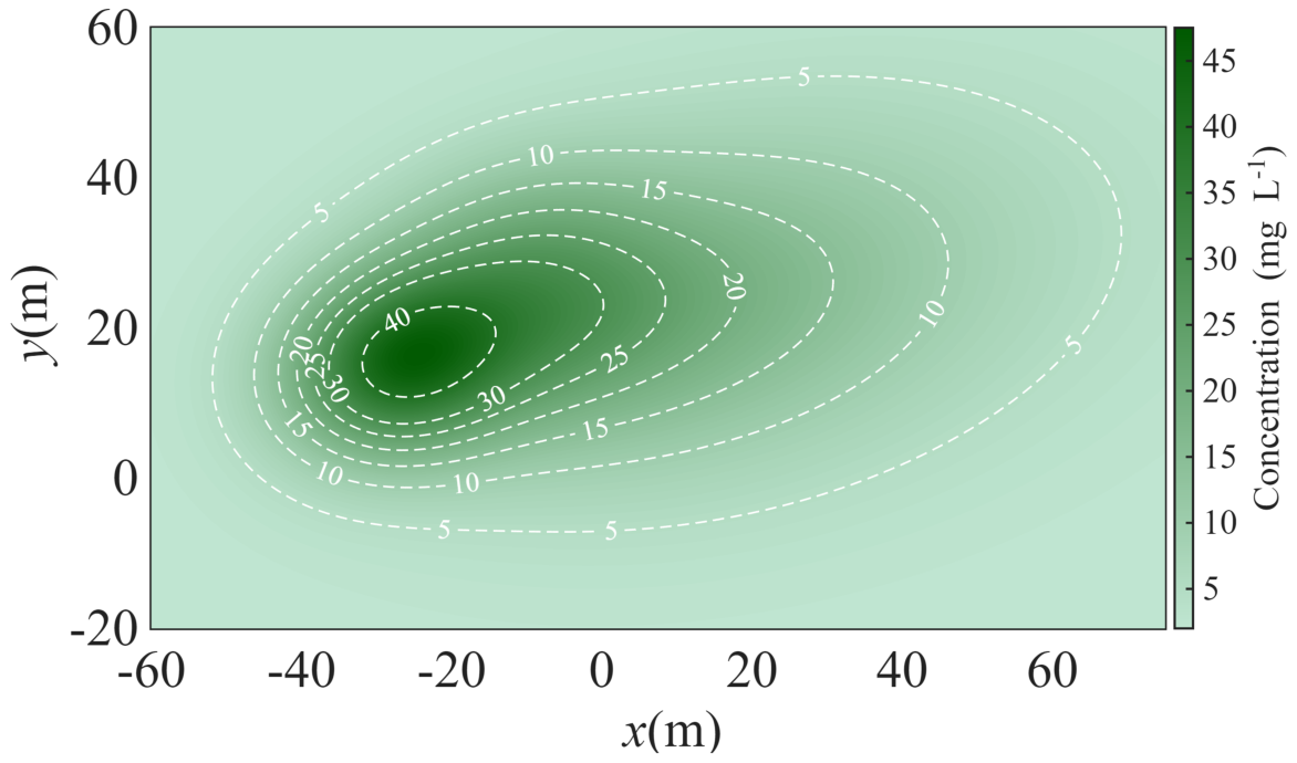
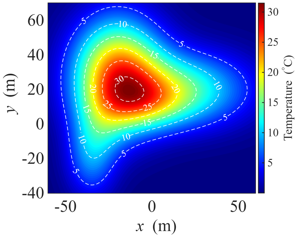
To evaluate the proposed method, a suspended particulate matter scalar field and a temperature field were selected as two representative unknown marine scalar-field scenarios. The suspended particulate matter concentration field represents a dredging-induced sediment plume, whose spatial distribution is characterized by the suspended particulate matter concentration [31]. The temperature field represents the spatial distribution of a marine thermal feature, motivated by AUV-based ocean-layer detection and tracking using in situ temperature measurements [11]. The spatial distributions of the two scalar fields are shown in Figure 2 and Figure 3, respectively.
The simulation model employed a fixed-step discrete solver with a sampling period of T s = 0.01 s, and the simulation duration was 200 s. The initial pose and velocity of the AUH were set as η h ( 0 ) = [ 8 , 3 , 3 π / 4 ] T and v h ( 0 ) = [ 0 , 0 , 0 ] T , respectively.
Time-varying model uncertainty and multi-frequency ocean-current disturbances [4], together with colored random measurement noise [32], were considered in the simulations. To account for the influence of parameter perturbations in practical marine environments, the model uncertainty was set as Δ ( t ) = 0.3 sin ( 0.3 t ) F h ( v h ) . The ocean-current disturbance acting on the horizontal-plane dynamics was selected as
d ( t ) = 0.3 sin ( 0.2 t ) + 0.1 sin ( 0.3 t ) , 0.2 cos ( 0.2 t ) + 0.3 cos ( 0.3 t ) , 0.1 sin ( t ) T .
The sensor measurement was affected by bounded colored random noise with temporal correlation. Let w [ k ] denote a bounded zero-mean random excitation satisfying w [ k ] [ N s , N s ] . The measurement noise was generated through two cascaded first-order correlated processes as
ξ n [ k ] = a 1 ξ n [ k 1 ] + ( 1 a 1 ) w [ k ] , n s [ k ] = a 2 n s [ k 1 ] + ( 1 a 2 ) ξ n [ k ] ,
where N s = 0.3 , a 1 = 0.985 , and a 2 = 0.970 . The initial states of the noise-generating process were set to zero. Consequently, | n s [ k ] | N s , which is consistent with the bounded-noise condition in Assumption 3, while the temporal correlation provided a smoothly varying random measurement-noise pattern.
The two scalar fields used in the simulations were twice continuously differentiable over the corresponding operating regions. Moreover, the AUH position trajectory generated by the dynamic model had bounded velocity and almost-everywhere bounded acceleration over the finite simulation interval. Therefore, the sufficient regularity condition stated after Assumption 3 was satisfied, and the resulting true scalar signal s ( t ) = F ( r ( t ) ) was differentiable with a Lipschitz-continuous rate. The colored random noise was added only to the measured scalar signal s m ( t ) and therefore did not alter the regularity of the true scalar signal s ( t ) .
The target scalar values were selected as s d , SPM = 20 mg L−1 and s d , T = 20 °C. The control and differentiator parameters used in the simulations are listed in Table 1.
The parameters in Table 1 were selected according to their respective roles in the closed-loop system.
The prescribed-performance parameters T c , , p, and κ were first specified according to the desired velocity-matching performance. In particular, and κ determine the explicit terminal bound e ¯ v = κ / 1 2 , which is then available for the gain conditions of the isoline-tracking subsystem. The gains k 2 and k 3 were selected according to the stability conditions and the desired scalar-tracking response, after which k 1 was chosen to satisfy Lemma 1 and Theorem 1 using the explicit bound e ¯ v and was further adjusted according to the desired tracking response.
The velocity-control gain k 4 was selected by balancing the velocity-matching response and control effort. The parameters T c , , and p determine the contraction time, terminal range, and transient shape of the performance boundary, respectively, while κ determines the scale between the mapped and physical velocity-matching errors. For the scalar-rate estimator, L s was conservatively selected according to the expected scalar-rate variation, γ d > L s was chosen with a sufficient margin, and T s together with k ¯ determines the available historical-data window. The desired cruising speed v d = 1 m s 1 was selected to represent the low-speed boundary-observation operation of the AUH.
The sampled differentiator directly uses the noisy scalar measurement. With k ¯ = 90 and T s = 0.01 s , the maximum historical-data window is T ¯ = k ¯ T s = 0.90 s , while the maximum increment of the differentiator output between two successive sampling instants is γ d T s = 0.05 .
At sampling instant k, let m k = min { k , k ¯ } . The implementation retains the current measurement and the most recent m k historical measurements so that, at most k ¯ + 1 = 91 , scalar samples are stored. The supremum search in Equation (31) was implemented on the sampling grid by setting T = i T s and σ = j T s , where i = 1 , , m k and j = 0 , , i . For each candidate pair, Q s [ k , i , j ] = s m [ k j ] s m [ k ] + s m [ k ] s m [ k i ] j / i was evaluated, and N ^ s [ k ] was obtained as one half of the maximum of | Q s [ k , i , j ] | L s T s 2 j ( i j ) / 2 over all admissible pairs. Thus, the continuous supremum was replaced by a finite exhaustive search over the stored measurements. The number of candidate evaluations at each sampling instant was m k ( m k + 3 ) / 2 , giving a computational complexity of O ( m k 2 ) and a memory requirement of O ( m k ) . With k ¯ = 90 , the maximum search involved 4185 candidate evaluations and 91 stored scalar samples per sampling instant.

4.1. Suspended Particulate Matter Concentration Field

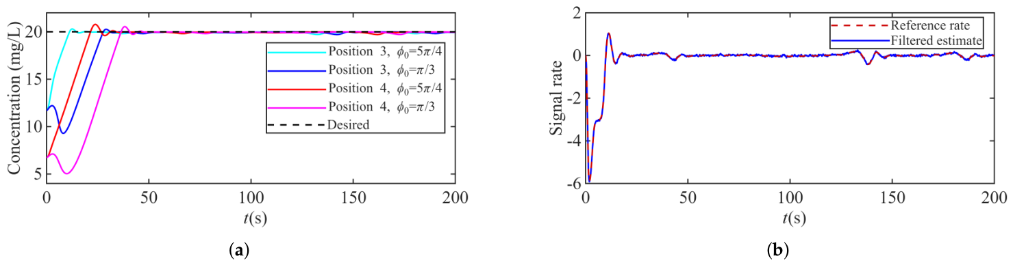
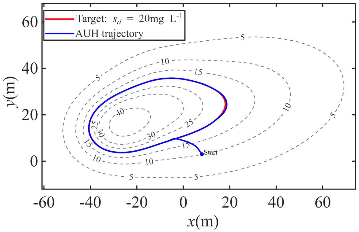
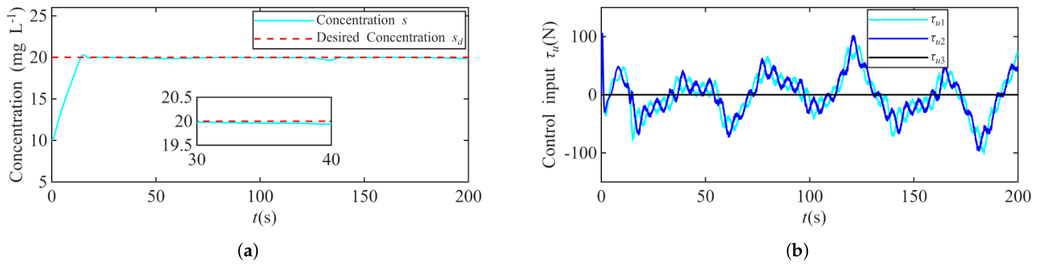
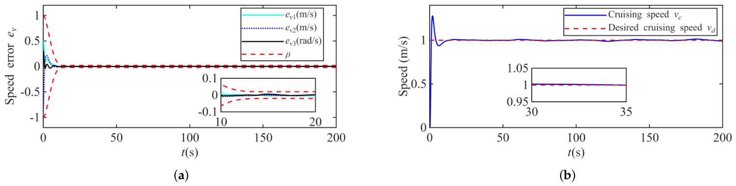
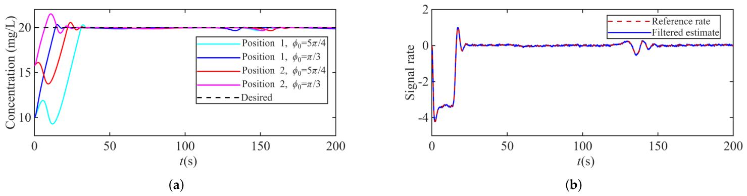
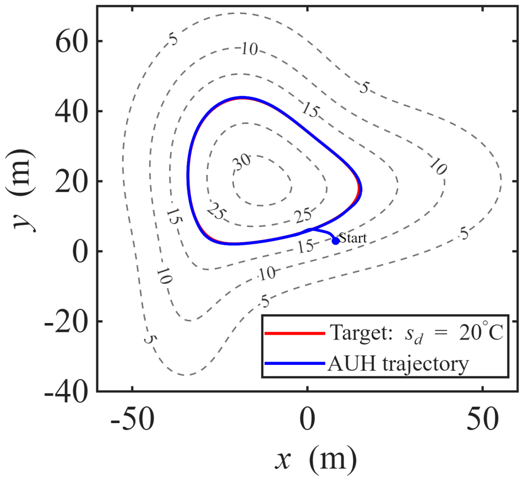
Delineating a prescribed suspended particulate matter concentration isoline provides a basis for assessing the plume-affected area and its dispersion trend. Figure 4, Figure 5 and Figure 6 show the AUH isoline-tracking trajectory, the concentration and thruster-input responses, and the velocity-matching results, respectively. Figure 7 presents the concentration responses under different initial poses and the scalar-rate estimation result under the adopted noise condition.
As shown in Figure 4, the AUH first adjusts its heading toward the plume boundary and then maintains continuous tangential motion along the 20 mg L 1 concentration isoline. The resulting trajectory closely follows the irregular closed isoline without prior knowledge of the plume geometry. Figure 5a shows that the measured concentration converges to a small neighborhood of the desired value. The larger initial control action in Figure 5b is associated with boundary approach and heading adjustment, after which the thruster inputs vary smoothly with small amplitudes. As shown in Figure 6a, the three velocity-matching errors remain within the shrinking performance boundaries and enter the prescribed terminal region before T c . The cruising speed in Figure 6b subsequently settles near v d , supporting sustained concentration-boundary observation.
Figure 7a further investigates the influence of different initial positions and heading angles on the isoline-tracking performance. For the cases with initial directed angles outside the feasible region D ϕ , the AUH first undergoes an additional heading-adjustment process to enter the admissible angular domain, after which the isoline-tracking behavior is guaranteed. The results demonstrate that the proposed method can achieve the desired concentration boundary observation under different initial conditions, while the initial angular deviation mainly affects the transient recovery process. In addition, Figure 7b shows that the filtered estimate closely follows the reference scalar rate under the adopted noise condition. The estimation error remains small, with an RMSE of 0.0213 and a maximum absolute error of 0.0808 , while the correlation coefficient reaches 0.9997 , quantitatively demonstrating the effectiveness of the proposed scalar-rate estimation scheme.

4.2. Temperature Field

Continuous observation along a temperature isoline reveals the spatial extent and evolution of marine thermal features. The AUH isoline-tracking trajectory, the temperature and thruster-input responses, and the velocity-matching results are presented in Figure 8, Figure 9 and Figure 10, respectively. Figure 11 further presents the temperature responses under different initial poses and the scalar-rate estimation result under the adopted noise condition.
Figure 8 shows that the AUH intercepts the 20 ° C isoline after the initial maneuver and subsequently follows its changing local direction throughout the closed thermal-feature boundary. The resulting path remains close to the prescribed temperature contour, demonstrating that the yaw motion is continuously adapted to the spatial variation of the temperature field.
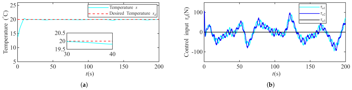
Figure 9a shows that the measured temperature reaches the vicinity of 20 ° C and remains there during the subsequent circumnavigation. Meanwhile, the thruster inputs in Figure 9b vary smoothly while providing the required directional corrections.
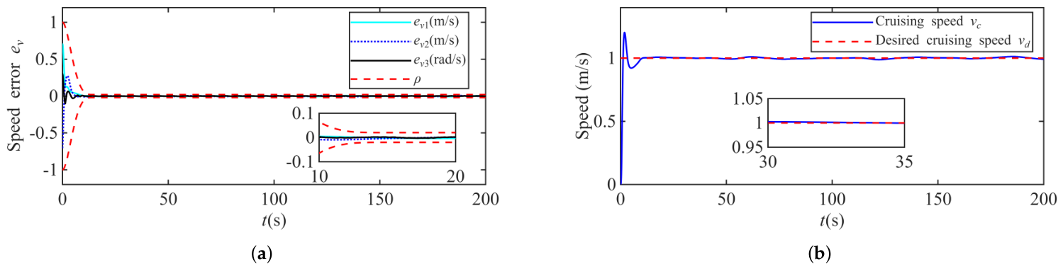
The prescribed-time behavior is further reflected in Figure 10a: the velocity errors contract with the performance boundaries and remain in the terminal range after T c . The cruising speed in Figure 10b follows v d without a persistent deviation, thereby supporting continuous observation along the thermal isoline.
Figure 11a shows that the temperature responses converge to the desired isoline under different initial poses. Figure 11b shows that the filtered estimate closely follows the reference scalar rate under the adopted noise condition. The estimation error remains small, with an RMSE of 0.02198 and a maximum absolute error of 0.07892 , while the correlation coefficient reaches 0.99960 , quantitatively demonstrating the effectiveness of the proposed scalar-rate estimation scheme.

4.3. Comparative Analysis

To further evaluate the advantages of the proposed method, comparisons with a conventional performance-function method and a forward-difference filtering method were conducted in the suspended particulate matter concentration field.
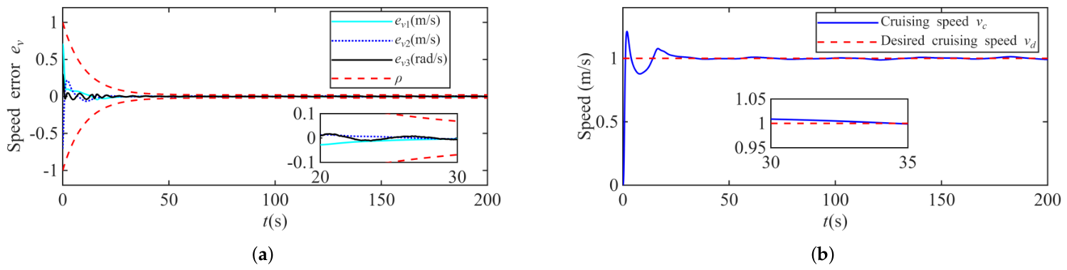
As shown in Figure 12, the conventional performance function can constrain the velocity-matching errors and eventually regulate the cruising speed toward v d . However, its error boundary decreases asymptotically, and the time required to reach a specified terminal accuracy cannot be explicitly assigned. In contrast, the prescribed-performance function adopted in this study directly specifies both the contraction time T c and the terminal error range, providing a more explicit transient-performance specification.
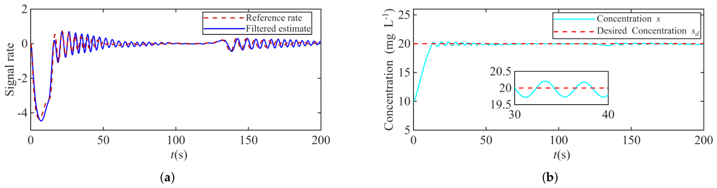
Figure 13b shows that the forward-difference filter produces noticeable oscillations and amplitude deviations in the scalar-rate estimate under measurement noise, particularly during rapid signal variations. These estimation fluctuations are propagated to the isoline regulation and result in more evident concentration oscillations around the desired value, as shown in Figure 13a. By comparison, the proposed rate-estimation method provides closer scalar-rate tracking with smaller fluctuations, thereby reducing the influence of differentiation noise on the subsequent isoline-control response.

4.4. Prospective Experimental Validation

To further evaluate the practical applicability of the proposed method, a two-stage experimental scheme consisting of controlled water-tank tests and subsequent marine trials is planned. In the water-tank stage, a spatially nonuniform scalar field can be generated using a controllable temperature or concentration distribution, and the AUH can be equipped with a local scalar sensor to obtain the measurements required by the proposed controller. The onboard implementation will execute the scalar-rate estimation, virtual yaw regulation, and prescribed-time velocity-matching controller using the same sampled-data structure as in the simulations. Different initial positions and headings can be tested, while the field distribution, AUH motion states, and thruster inputs are recorded independently for performance evaluation. The main evaluation indices will include the scalar-tracking error, cruising-speed error, scalar-rate estimation accuracy, convergence behavior, and control-input variation.
After the controlled experiments, marine trials can be conducted in a naturally varying temperature field or suspended particulate matter region. During these trials, only the locally measured scalar value and the onboard motion states required by the proposed control framework will be used for real-time control, without prior reconstruction of the global scalar field or target-isoline geometry. Independent positioning and environmental survey information can be recorded solely as reference data for offline evaluation of the actual isoline-tracking trajectory. The field tests will focus on examining the influence of realistic ocean-current disturbances, sensor noise, spatial field variation, and finite thruster capability on the scalar-rate estimation and isoline-tracking performance. This progressive validation procedure will provide a practical basis for assessing the proposed method under increasingly realistic marine conditions.
In summary, the two marine scalar-field observation scenarios demonstrate that the proposed AUH isoline-tracking control method is applicable to suspended particulate matter concentration and temperature fields with different spatial distributions and isoline geometries. Under time-varying model uncertainty, multi-frequency ocean-current disturbances, and bounded colored measurement noise, the AUH approaches and continuously tracks the prescribed isoline while maintaining the desired cruising speed and the velocity-matching errors within the prescribed performance boundaries. The simulations with different initial poses further demonstrate the recovery and tracking capability under different initial conditions, while the quantitative scalar-rate estimation results show small estimation errors and high correlation with the reference rate in both scalar fields. Furthermore, the comparative analysis in the suspended particulate matter concentration field shows that the proposed prescribed-time performance function provides an explicit specification of the error-contraction time and terminal range, while the proposed scalar-rate estimation scheme reduces the estimation fluctuations and their influence on the isoline-tracking response compared with the forward-difference filtering method. These results collectively demonstrate the effectiveness and applicability of the proposed framework for isoline observation in different unknown marine scalar fields under the considered disturbances and measurement noise.

5. Conclusions

This study provides an AUH isoline-tracking framework for continuous boundary observation in unknown marine scalar fields using only noisy local measurements. The proposed isoline kinematic relation enables the AUH to approach a prescribed scalar level and maintain tangential motion without reconstructing the global field or exactly compensating for the unknown spatial-field coupling. The online scalar-rate estimation scheme provides reliable rate information from noisy scalar measurements, while the low-complexity prescribed-time velocity-matching controller constrains the velocity-matching errors within the prescribed performance boundary without imposing an upper bound on finite initial velocity errors. Simulations in suspended particulate matter concentration and temperature fields demonstrate the applicability of the proposed framework to marine scalar-boundary observation under disturbances and measurement noise.
The present study considers two-dimensional scalar fields and ideal realization of the commanded control input. Future work will extend the framework to spatiotemporally varying three-dimensional marine scalar fields. Furthermore, the proposed framework will be validated through tank experiments and sea trials under realistic sensing and environmental conditions.

Author Contributions

Conceptualization, Z.W. and Y.Z.; methodology, Z.W. and Y.Z.; software, Z.W. and Y.Z.; validation, W.K.; formal analysis, Y.Z.; investigation, Z.W.; resources, W.K.; writing—original draft preparation, Y.Z.; writing—review and editing, Z.W. and W.K.; visualization, Z.W. and Y.Z.; supervision, Z.W.; funding acquisition, W.K. and Z.W. All authors have read and agreed to the published version of the manuscript.

Funding

This work was supported by the Fundamental Research Funds for the Central Universities (JUSRP202601008).

Institutional Review Board Statement

Not applicable.

Informed Consent Statement

Not applicable.

Data Availability Statement

The data generated or analyzed during the current study are available from the corresponding author upon reasonable request. The materials and code used during the current study are also available from the corresponding author upon reasonable request.

Conflicts of Interest

Author Wuchen Kang was employed by the company SINOPEC Research Institute of Petroleum Engineering Co., Ltd. The remaining authors declare that the research was conducted in the absence of any commercial or financial relationships that could be construed as a potential conflict of interest.

Appendix A. Proof of the Positive Invariance of the Angular Region

Proof of Lemma 1.
Define
λ ϕ = v d γ 1 cos ε ϕ k 2 > 0 .
For t T c , Theorem 3 and Equation (50) give | e v , 3 ( t ) | < e ¯ v .
First, consider the lower boundary ϕ = ε ϕ . From Equations (12) and (18), one obtains
e p = v d g ( r ) cos ε ϕ + k 2 tanh e s k 3 v d γ 1 cos ε ϕ k 2 = λ ϕ > 0 .
Using ω = ω d + e v , 3 , Equation (19) together with Equation (24) gives
ϕ ˙ v d γ 3 γ 1 + k 1 λ ϕ e ¯ v .
It follows from Equation (25) that
k 1 λ ϕ > v d γ 3 γ 1 + e ¯ v .
Therefore, at ϕ = ε ϕ , ϕ ˙ > 0 .
Next, consider the upper boundary ϕ = π ε ϕ . Since cos ( π ε ϕ ) = cos ε ϕ , it similarly follows that
e p = v d g ( r ) cos ε ϕ + k 2 tanh e s k 3 v d γ 1 cos ε ϕ + k 2 = λ ϕ < 0 .
Thus, ω d k 1 λ ϕ , and
ϕ ˙ v d γ 3 γ 1 k 1 λ ϕ + e ¯ v < 0 .
Thus, ϕ ˙ > 0 at the lower boundary, and ϕ ˙ < 0 at the upper boundary. The closed-loop vector field at both boundaries points toward the interior of D ϕ . If ϕ ( T c ) D ϕ , then ϕ ( t ) D ϕ for all t T c . □

Appendix B. Proof of the Ultimate Bounds on the Scalar-Tracking Error and Directed Angle

Proof of Theorem 1.
Rewrite Equation (21) as
e ˙ p = a ( t ) e p + d F ( t ) ,
where
a ( t ) = k 1 v d g ( r ) sin ϕ , d F ( t ) = v d g ( r ) sin ϕ e v , 3 + v d 2 h T ( ψ ) 2 F ( r ) h ( ψ ) + k 2 k 3 sech 2 e s k 3 e ˙ s .
By Lemma 1, ϕ ( t ) D ϕ for t T c , and hence sin ϕ sin ε ϕ > 0 . Combining this result with g ( r ) γ 1 gives
a ( t ) k 1 v d γ 1 sin ε ϕ a p > 0 .
According to Equation (12) and g ( r ) γ 2 ,
| e ˙ s | = | s ˙ | v d γ 2 .
Moreover, since h ( ψ ) = 1 and 2 F ( r ) γ 3 ,
h T ( ψ ) 2 F ( r ) h ( ψ ) γ 3 .
It follows that
| d F ( t ) | v d 2 γ 3 + k 2 k 3 v d γ 2 + v d γ 2 e ¯ v B F .
Select the Lyapunov function
V p = 1 2 e p 2 .
Taking its derivative along Equation (21) gives
V ˙ p = e p e ˙ p a p e p 2 + B F | e p | = a p | e p | | e p | B F a p .
Noting that
B F a p = v d γ 3 + ( k 2 / k 3 ) γ 2 + γ 2 e ¯ v k 1 γ 1 sin ε ϕ = η p ,
one obtains
lim sup t | e p ( t ) | η p .
The first lower-bound condition implied by Equation (26) ensures that η p < k 2 . For any constant δ satisfying 0 < δ < k 2 η p , there exists T δ T c such that
| e p ( t ) | η p + δ , t T δ .
From the definition of the composite error in Equation (18),
e ˙ s = k 2 tanh e s k 3 + e p .
Select V s = e s 2 / 2 . For any t T δ ,
V ˙ s = e s e ˙ s k 2 | e s | tanh | e s | k 3 + ( η p + δ ) | e s | = | e s | k 2 tanh | e s | k 3 η p δ .
Therefore, when
| e s | > k 3 atanh η p + δ k 2 ,
one has V ˙ s < 0 , which yields
lim sup t | e s ( t ) | k 3 atanh η p + δ k 2 .
Letting δ 0 + and using e s = s s d give
lim sup t | s ( t ) s d | k 3 atanh η p k 2 .
Furthermore, Equation (18) gives
s ˙ = e p k 2 tanh e s k 3 .
Together with the above ultimate bounds, this relation yields
lim sup t k 2 tanh e s ( t ) k 3 η p .
Therefore,
lim sup t | s ˙ ( t ) | 2 η p .
According to Equation (12) and g ( r ) γ 1 ,
| cos ϕ ( t ) | = | s ˙ ( t ) | v d g ( r ) | s ˙ ( t ) | v d γ 1 ,
and hence
lim sup t | cos ϕ ( t ) | 2 η p v d γ 1 .
By Lemma 1, ϕ ( t ) [ ε ϕ , π ε ϕ ] , and thus
| cos ϕ ( t ) | = sin ϕ ( t ) π 2 .
In addition, Equation (26) ensures that
2 η p v d γ 1 < 1 .
Using the monotonicity of the inverse sine function on [ 0 , 1 ) gives
lim sup t ϕ ( t ) π 2 arcsin 2 η p v d γ 1 .
Therefore, Equation (27) holds. □

Appendix C. Proof of the Continuous-Time Differentiator Properties

Proof of Theorem 2.
Since the right-hand side of Equation (35) is uniformly bounded, s ˙ ^ ( t ) , as a Filippov solution, is absolutely continuous on every compact time interval. Moreover, since Sgn ( x ) [ 1 , 1 ] , it follows directly from Equation (35) that
d d t s ˙ ^ ( t ) γ d a . e .
Therefore, s ˙ ^ ( t ) is Lipschitz continuous, with a Lipschitz constant not exceeding γ d .
The scalar-rate estimation error is considered next. Define the estimation error of the regularized raw differentiator and that of the final differentiator as
e m ( t ) = y m ( t ) s ˙ ( t ) , e d ( t ) = s ˙ ^ ( t ) s ˙ ( t ) ,
respectively. Under Assumption 3 and N s < L s T ¯ 2 / 2 , the worst-case error property of the regularized raw differentiator ([14], Proposition 1) gives
T ˜ s = 2 N s L s , E s = 2 2 N s L s ,
and
| e m ( t ) | E s , t T ˜ s .
Since s ˙ ^ y m = e d e m , it follows from Equation (35) that there exists, almost everywhere, a function μ d ( t ) satisfying
μ d ( t ) Sgn e d ( t ) e m ( t ) ,
such that the final differentiation-error dynamics are
e ˙ d ( t ) = γ d μ d ( t ) s ¨ ( t ) .
Since | μ d ( t ) | 1 and | s ¨ ( t ) | L s almost everywhere, Equation (A35) gives
| e ˙ d ( t ) | γ d + L s a . e .
According to s ˙ ^ ( 0 ) = y m ( 0 ) = 0 and | s ˙ ( 0 ) | R 1 , one has | e d ( 0 ) | R 1 . Hence,
| e d ( t ) | R 1 + γ d + L s t , 0 t T ˜ s .
For t > T ˜ s , select
V d ( t ) = | e d ( t ) | .
When V d ( t ) > E s , Equation (A33) implies
| e d ( t ) | > | e m ( t ) | .
Therefore,
sgn e d ( t ) e m ( t ) = sgn e d ( t ) .
Combining this relation with Equation (A35) yields
V ˙ d ( t ) = sgn ( e d ) e ˙ d = γ d sgn ( e d ) sgn ( e d e m ) s ¨ sgn ( e d ) γ d + L s = γ d L s < 0
almost everywhere. Thus, whenever | e d ( t ) | > E s , the final differentiation error approaches the error region | e d | E s at a rate of at least γ d L s .
A contradiction argument is used to show that the estimation error remains in this region after the time T d defined by Equation (36). Suppose that there exists t 1 T d such that
V d ( t 1 ) > E s .
Let ( a , b ) be the connected interval containing t 1 in the set
t T ˜ s | V d ( t ) > E s .
If a > T ˜ s , the continuity of V d ( t ) gives V d ( a ) = E s . Integrating over ( a , t 1 ] yields
V d ( t 1 ) V d ( a ) γ d L s ( t 1 a ) < E s ,
which contradicts V d ( t 1 ) > E s .
If a = T ˜ s , then Equation (A37) gives
V d ( T ˜ s ) R 1 + γ d + L s T ˜ s .
Integrating over [ T ˜ s , t 1 ] , using t 1 T d , and applying Equation (36) give
V d ( t 1 ) V d ( T ˜ s ) γ d L s t 1 T ˜ s R 1 + γ d + L s T ˜ s γ d L s T d T ˜ s = 2 L s T ˜ s = 2 2 N s L s = E s ,
which again contradicts V d ( t 1 ) > E s .
Consequently,
| e d ( t ) | E s , t T d ,
which proves Equation (37). The definition of T d in Equation (36) follows from the preceding reaching-time analysis.
When N s = 0 , one has T ˜ s = 0 and E s = 0 . In the noise-free case, the regularized raw differentiator satisfies e m ( t ) = 0 . The preceding analysis then gives
T d = R 1 γ d L s , e d ( t ) = 0 , t T d .
Therefore, the differentiator exactly recovers the true scalar value rate after a finite time. □

Appendix D. Proof of the Positive Invariance of the Velocity- Performance Boundary

Proof of Theorem 3.
It follows from Equations (39) and (52) that
e ˙ v = d v ( t ) + J ( ψ ) M 1 G 0 τ u .
Substituting the controller in Equation (53) into Equation (A49) and using J ( ψ ) J T ( ψ ) = I give
e ˙ v = d v ( t ) k 4 ε v ( t ) .
Differentiating Equation (47), the ith component of the normalized velocity error satisfies
z ˙ i = N ( e v , i ) ρ ( t ) d v , i ( t ) k 4 ε v , i ( t ) ρ ˙ ( t ) ρ ( t ) z i ( t ) .
Since 0 < ρ ( t ) 1 , it follows from Equation (45) that ρ ˙ ( t ) / ρ ( t ) is bounded. Moreover, Equation (41) gives
0 < N ( e v , i ) = κ e v , i 2 + κ 3 / 2 1 κ .
Together with Assumption 4, these results show that all terms in Equation (A51), except ε v , i ( t ) , are bounded.
According to Equation (48), z i ( 0 ) ( 1 , 1 ) . Suppose, by contradiction, that Equation (56) does not hold. Then, there exists a finite first boundary-reaching time t f > 0 at which one component satisfies
| z i ( t ) | < 1 , 0 t < t f , lim t t f | z i ( t ) | = 1 .
First, consider
lim t t f z i ( t ) = 1 .
Since t f > 0 , the performance function satisfies 0 < ρ ( t f ) < 1 . Let ρ f = ρ ( t f ) . From X ( e v , i ) = ρ ( t ) z i , one obtains
X ( e v , i ) ρ f as z i 1 .
Using the inverse mapping in Equation (42) gives
e v , i κ ρ f 1 ρ f 2 ,
and hence
N ( e v , i ) ρ ( t ) 1 ρ f 2 3 / 2 κ ρ f > 0 .
On the other hand, Equation (51) shows that
ε v , i + as z i 1 .
Therefore, Equation (A51) yields
lim t t f z ˙ i ( t ) = .
Thus, there exists a left neighborhood of t f in which z ˙ i ( t ) < 0 . Consequently, z i ( t ) is strictly decreasing as it approaches t f and cannot approach the upper boundary z i = 1 from the region z i < 1 , which produces a contradiction.
Next, consider
lim t t f z i ( t ) = 1 .
In this case,
X ( e v , i ) ρ f , e v , i κ ρ f 1 ρ f 2 ,
and
N ( e v , i ) ρ ( t ) 1 ρ f 2 3 / 2 κ ρ f > 0 .
According to Equation (51),
ε v , i as z i 1 + .
It follows from Equation (A51) that
lim t t f z ˙ i ( t ) = + .
Hence, there exists a left neighborhood of t f in which z ˙ i ( t ) > 0 . Therefore, z i ( t ) is strictly increasing as it approaches t f and cannot approach the lower boundary z i = 1 from the region z i > 1 , which again produces a contradiction.
No finite first boundary-reaching time exists. Therefore, Equation (56) holds. Combining this result with Equations (42), (43), (49), and (50) completes the proof. □

References

  1. Leite, P.N.; Pereira, P.N.; Dionísio, J.M.M.; Pinto, A.M. Hybrid underwater imaging for the tri-dimensional inspection of critical structural elements in offshore platforms. Ocean Eng. 2024, 314, 119658. [Google Scholar] [CrossRef] [Scilit]
  2. Aguzzi, J.; Thomsen, L.; Flögel, S.; Robinson, N.J.; Picardi, G.; Chatzievangelou, D.; Bahamon, N.; Stefanni, S.; Grinyó, J.; Fanelli, E.; et al. New technologies for monitoring and upscaling marine ecosystem restoration in deep-sea environments. Engineering 2024, 34, 195–211. [Google Scholar] [CrossRef] [Scilit]
  3. An, X.; Shi, H.; Li, H.; Xing, H.; Gu, Y.; Huang, H.; Chen, Y. Autonomous underwater helicopter-HY-1: Design and field trials of a seabed operational vehicle. J. Field Robot. 2026, 43, 969–994. [Google Scholar] [CrossRef] [Scilit]
  4. Zang, Y.; Wu, Z.; Huang, H.; Fan, Q. Low-complexity trajectory tracking control of an AUH with unknown control directions and asymmetric velocity constraints. Ocean Eng. 2026, 358, 125717. [Google Scholar] [CrossRef] [Scilit]
  5. Zhang, Y.; Li, S. An incremental physics-informed neural network for rapid prediction of suspended sediment plume for deep-sea mining. J. Process Control 2026, 157, 103604. [Google Scholar] [CrossRef] [Scilit]
  6. Matveev, A.S.; Berman, I.; Bugrova, A.; Bystramovich, M.; Kapitonov, A.A.; Manaenko, V. Nongradient-based tracking of environmental field isolines in a changing medium by Dubins-vehicle type robots. IEEE Trans. Autom. Control 2024, 69, 952–967. [Google Scholar] [CrossRef] [Scilit]
  7. Cao, Y.; Shi, Y.; Song, Y.; Huang, Q.; Pan, G. Event-triggered prescribed performance control for safety-aware and resource-efficient isoline tracking of autonomous underwater vehicle. Ocean Eng. 2026, 349, 123918. [Google Scholar] [CrossRef] [Scilit]
  8. Tian, Z.; Zheng, H.; Wu, W.; Xu, W. Integrated front reconstruction and AUV tracking control with Bayesian optimization and NMPC. Ocean Eng. 2025, 326, 120761. [Google Scholar] [CrossRef] [Scilit]
  9. Mo-Bjørkelund, T.; Mendes, R.; López-Castejón, F.J.; Ludvigsen, M. Adaptive ocean gradient tracking using an autonomous underwater vehicle with a boundless model. IEEE J. Ocean. Eng. 2025, 50, 955–967. [Google Scholar] [CrossRef] [Scilit]
  10. Zhang, Y.; Li, S. Dynamic boundary estimation of suspended sediment plume benefit by the autonomous underwater vehicle sensing. Sensors 2024, 24, 8182. [Google Scholar] [CrossRef] [Scilit]
  11. von See, T.B.; Greinert, J.; Meurer, T. Detection and tracking of ocean layers using an AUV with UKF-based extremum-seeking control in the Baltic Sea. Sci. Rep. 2024, 14, 20629. [Google Scholar] [CrossRef] [Scilit]
  12. Song, Y.; Huang, B.; Zhu, C.; Cheng, B. Safety-aware isoline tracking control for unmanned surface vehicle. Ocean Eng. 2025, 327, 120910. [Google Scholar] [CrossRef] [Scilit]
  13. Calmbach, B.; Moreno, J.A.; Reger, J. Minimizing the homogeneous L2-gain of homogeneous differentiators. Eur. J. Control 2024, 80, 101039. [Google Scholar] [CrossRef] [Scilit]
  14. Aldana-López, R.; Seeber, R.; Haimovich, H.; Gómez-Gutiérrez, D. Optimal robust exact first-order differentiators with Lipschitz-continuous output. IEEE Trans. Autom. Control 2025, 70, 6191–6198. [Google Scholar] [CrossRef] [Scilit]
  15. Seeber, R. Proper implicit discretization of arbitrary-order robust exact differentiators—Without and with noise filtering. Int. J. Robust. Nonlinear Control 2025, 35, 7860–7880. [Google Scholar] [CrossRef] [Scilit]
  16. Lin, J.; Sun, J.; Yan, H.; Su, G. Active disturbance rejection control for systems with uncertainties and noise using super-twisting-differentiator-based event-triggered ESO. Int. J. Syst. Sci. 2025, 56, 982–995. [Google Scholar] [CrossRef] [Scilit]
  17. Guo, Y.; Su, T.; Sheng, C.; Lu, X.; Wang, H.; Su, X. Enhanced ADRC using tracking differentiator with phase compensation to strengthen the ability of measurement noise suppression. IEEE Trans. Instrum. Meas. 2025, 74, 3004613. [Google Scholar] [CrossRef] [Scilit]
  18. Liu, Y.; An, S.; Wang, L.; Fan, Z. Predefined-time sliding-mode tracking control of autonomous underwater vehicles with uncertainties and disturbances. Ocean Eng. 2025, 331, 121318. [Google Scholar] [CrossRef] [Scilit]
  19. Sui, B.; Zhang, J.; Liu, Z. Extended-state-observer-based prescribed-time trajectory tracking control for USV with prescribed performance constraints and input saturation. Ocean Eng. 2025, 316, 120005. [Google Scholar] [CrossRef] [Scilit]
  20. Chen, Y.; Kong, M.; Zhao, Z.; Dong, J.; Li, R. Adaptive disturbance-observer-based fixed-time sliding-mode tracking control for autonomous surface vehicles with prescribed performance. Ocean Eng. 2025, 341, 122427. [Google Scholar] [CrossRef] [Scilit]
  21. Fan, Z.; Wang, L.; Meng, H.; Yang, C. Reinforcement-learning-based predefined-time control for USV trajectory tracking under disturbance and input saturation. Ocean Eng. 2025, 342, 122917. [Google Scholar] [CrossRef] [Scilit]
  22. Xia, Y.; He, J.; Lendek, Z.; Rudas, I.J.; Agarwal, R.K. Global singularity-free prescribed performance control for faulty nonlinear systems via parameterized nonmonotonic constraints. IEEE/CAA J. Autom. Sin. 2026, 13, 1176–1183. [Google Scholar] [CrossRef] [Scilit]
  23. Wu, Z.; Wang, S.; Shao, X.; Liu, F.; Bao, Z. Adaptive path planning for subsurface plume tracing with an autonomous underwater vehicle. Robotics 2024, 13, 132. [Google Scholar] [CrossRef] [Scilit]
  24. Jiu, H.; Deng, W. A planning method for chemical plume tracking and source localization with autonomous underwater vehicle. Int. J. Adv. Robot. Syst. 2024, 21, 17298806241233909. [Google Scholar] [CrossRef] [Scilit]
  25. Yan, Z.; Min, X.; Xu, D.; Geng, D. A novel method for underactuated UUV tracking unknown contour based on forward-looking sonar. Ocean Eng. 2024, 301, 117545. [Google Scholar] [CrossRef] [Scilit]
  26. Seeber, R.; Haimovich, H. Optimal robust exact differentiation via linear adaptive techniques. Automatica 2023, 148, 110725. [Google Scholar] [CrossRef] [Scilit]
  27. Wu, Z.; Song, Z.; Huang, H. Prescribed-performance-based formation control for multiple autonomous underwater helicopters with complex dynamic characteristics. J. Mar. Sci. Eng. 2024, 12, 2246. [Google Scholar] [CrossRef] [Scilit]
  28. Zhang, Z.; Lin, M.; Li, D.; Lin, R. Gaze-assisted prescribed performance controller for AUV trajectory tracking in time-varying currents. J. Mar. Sci. Eng. 2024, 12, 1643. [Google Scholar] [CrossRef] [Scilit]
  29. Dai, M.; Cai, W.; He, C.; Shi, H.; Zhou, X. Event-triggered prescribed-time position control for AUVs with input constraints: A nonlinear disturbance observer approach. Intell. Mar. Technol. Syst. 2026, 4, 8. [Google Scholar] [CrossRef] [Scilit]
  30. Wu, Z.; Wang, Q.; Huang, H. Adaptive neural networks trajectory tracking control for autonomous underwater helicopters with prescribed performance. Ocean Eng. 2022, 264, 112519. [Google Scholar] [CrossRef] [Scilit]
  31. von See, T.B.; Greinert, J.; Meurer, T. Multi-AUV sediment plume estimation using Bayesian optimization. Front. Mar. Sci. 2025, 11, 1504099. [Google Scholar] [CrossRef] [Scilit]
  32. Xu, Y.; Yang, R.; Zhuang, Y.; Liu, K.; Wang, K.; Chen, X.; Sun, M. Expectation–maximization-based Kalman filter under colored measurement noise for INS-based integrated human localization. Mech. Syst. Signal Process. 2025, 228, 112461. [Google Scholar] [CrossRef] [Scilit]
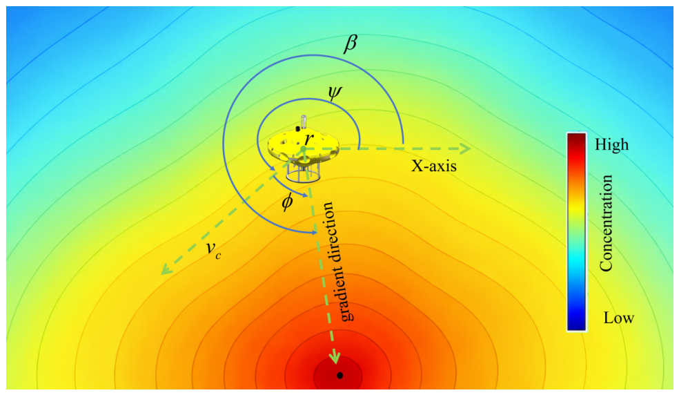
Figure 1. Schematic diagram of the geometric relationship for AUH isoline tracking in an unknown marine scalar field.
Electronics 15 04129 g001
Figure 2. Spatial distribution of the suspended particulate matter concentration field.
Electronics 15 04129 g002
Figure 3. Spatial distribution of the temperature field.
Electronics 15 04129 g003
Figure 4. AUH isoline-tracking trajectory in the suspended particulate matter concentration field.
Electronics 15 04129 g004
Figure 5. Concentration response and control inputs in the suspended particulate matter concentration field: (a) actual and desired concentrations; (b) thruster control inputs.
Electronics 15 04129 g005
Figure 6. Velocity-matching results in the suspended particulate matter concentration field: (a) velocity-matching errors and prescribed performance boundaries; (b) actual and desired cruising speeds.
Electronics 15 04129 g006
Figure 7. Concentration responses and scalar-rate estimation results in the suspended particulate matter concentration field: (a) concentration responses under different initial poses; (b) reference scalar rate and filtered estimate under the adopted noise condition.
Electronics 15 04129 g007
Figure 8. AUH isoline-tracking trajectory in the temperature field.
Electronics 15 04129 g008
Figure 9. Temperature response and control inputs in the temperature field: (a) actual and desired temperatures; (b) thruster control inputs.
Electronics 15 04129 g009
Figure 10. Velocity-matching results in the temperature field: (a) velocity-matching errors and prescribed performance boundaries; (b) actual and desired cruising speeds.
Electronics 15 04129 g010
Figure 11. Temperature responses and scalar-rate estimation results in the temperature field: (a) temperature responses under different initial poses; (b) reference scalar rate and filtered estimate under the adopted noise condition.
Electronics 15 04129 g011
Figure 12. Results of the conventional performance function without a prescribed convergence time: (a) velocity-matching errors and performance boundaries; (b) actual and desired cruising speeds.
Electronics 15 04129 g012
Figure 13. Results from the forward-difference filtering method under the adopted noise condition: (a) actual and desired concentrations; (b) reference scalar rate and filtered estimate.
Electronics 15 04129 g013
Table 1. Control and differentiator parameters used in the simulations.
ParameterValueParameterValue
k 1 0.1 k 2 3
k 3 2 k 4 2
v d 1 m s 1 κ 0.9
T c 15 s 0.02
p4 T s 0.01 s
L s 1 γ d 5
k 0 0 k ¯ 90
Disclaimer/Publisher’s Note: The statements, opinions and data contained in all publications are solely those of the individual author(s) and contributor(s) and not of MDPI and/or the editor(s). MDPI and/or the editor(s) disclaim responsibility for any injury to people or property resulting from any ideas, methods, instructions or products referred to in the content.