Pyramid Target Perception Network with Efficient Context Modeling and Multi-Scale Cross-Attention for Infrared Small Target Detection

Abstract

Infrared small target detection (IRSTD) is a challenging task in intelligent infrared sensing and electronic imaging systems, because dim targets often occupy only a few pixels and are easily disturbed by clutter, noise, and low-contrast background structures. A practical detector should preserve pixel-level target cues while suppressing target-like false responses. This paper proposes a Pyramid Target Perception Network (PTPN) for single-frame pixel-level IRSTD. The network integrates three complementary components: an Efficient Context Modeling (ECM) encoder employing 7 × 7 depthwise separable convolution for lightweight contextual feature extraction, a multi-scale target cross-attention (MTCA) module for hierarchical feature interaction, and a small-target feature pyramid network (STFPN) for target-preserving multi-scale aggregation. In addition, a physics-constrained loss (PCL) is introduced during training to regularize predictions according to infrared imaging characteristics, including point spread consistency, target-region relative intensity consistency, and signal-to-noise-ratio-aware separability. Experiments on IRSTD-1k, NUAA-SIRST, and NUDT-SIRST demonstrate that PTPN achieves $IoU$ scores of 71.87%, 79.56%, and 86.47%, respectively, with 4.55M parameters, 4.96G FLOPs at an input resolution of 256 × 256, and an inference speed of 45.0 FPS. Although PTPN achieves competitive overall performance, it does not attain the highest $IoU$ on NUDT-SIRST, indicating that pixel-level target-region estimation under complex scenes remains an area for further improvement. Overall, PTPN provides an effective balance between target localization, false-alarm suppression, and computational efficiency, supporting its potential application in AI-driven infrared image processing and intelligent electronic sensing systems.

1. Introduction

Infrared small target detection (IRSTD) aims to identify dim and spatially compact targets in infrared images. As a key component of infrared search and tracking systems, it has been widely studied for long-range early warning, maritime surveillance, aerospace observation, and guidance-related remote-sensing applications [1,2,3]. Unlike generic object segmentation, IRSTD usually deals with targets that occupy only a few pixels and provide limited shape, texture, or semantic information [4]. In real aerial, maritime, and ground scenes, cloud edges, sea clutter, terrain radiation, and sensor noise may produce responses that resemble true targets, which makes missed detections and false alarms difficult to avoid [5,6,7].

The main difficulty of IRSTD lies in the imbalance between weak target evidence and strong background interference. On the one hand, repeated feature downsampling may quickly dilute pixel-level target responses. On the other hand, enlarging the contextual range is necessary for distinguishing small targets from structured clutter. Existing methods have explored this problem from several perspectives. Traditional model-driven algorithms rely on background smoothness, local contrast, sparsity, or low-rank assumptions [8,9,10,11,12,13]. CNN-based segmentation networks improve feature learning and multi-level aggregation [14,15,16,17,18,19,20], while contrast-enhanced, shape-biased, and large-kernel designs further enrich target representation and contextual perception [21,22,23]. Transformer and attention-based methods further introduce long-range dependency modeling [24,25,26,27]. More recently, frequency-domain analysis, imaging priors, and hybrid learning strategies have been investigated to improve robustness under complex backgrounds and low-SNR conditions [28,29,30,31,32,33,34,35,36,37,38,39]. Recent IRSTD studies have further explored large-kernel contextual modeling [40], state-space/Mamba architectures [41], and diffusion-based formulations [42], extending the methodological landscape toward broader contextual perception, efficient long-range dependency modeling, and generative target prediction.

Although these studies have substantially advanced IRSTD, preserving weak target evidence throughout hierarchical representation learning remains challenging. Repeated downsampling may attenuate pixel-level target responses, whereas insufficient contextual information makes it difficult to distinguish true targets from target-like background structures. Attention-based models improve long-range or cross-scale interaction, but their effectiveness depends on how complementary information is selected across feature levels, particularly when most tokens correspond to background regions. Meanwhile, feature aggregation and imaging-related priors are often introduced as separate mechanisms, leaving the interaction among contextual modeling, cross-scale information exchange, weak-target propagation, and prediction regularization insufficiently coordinated. Therefore, rather than optimizing these stages independently, an effective IRSTD framework should maintain target evidence throughout the complete representation process while simultaneously suppressing background interference.

To address these coupled challenges, we develop a Pyramid Target Perception Network (PTPN) from a unified representation perspective. Rather than relying on a single isolated architectural mechanism, PTPN coordinates contextual modeling, cross-scale interaction, target-preserving pyramid propagation, and imaging-inspired supervision within a progressive detection pipeline. Specifically, the ECM encoder employs efficient 7 × 7 depthwise separable operations and residual feature transformation to capture surrounding context while retaining weak local responses. The MTCA module then enables features at each scale to selectively retrieve complementary information from a shared multi-scale context. Based on the enhanced representations, STFPN strengthens weak target responses and propagates semantic and localization information through bidirectional pyramid fusion and refinement. Finally, PCL provides complementary training constraints based on point-spread consistency, relative-intensity consistency, and target–background separability. Together, these components form a context–interaction–aggregation–supervision pipeline aimed at maintaining weak-target evidence throughout hierarchical representation learning rather than treating individual stages independently.

The main contributions of this paper are summarized as follows:

(1) We develop a unified Pyramid Target Perception Network (PTPN) for pixel-level infrared small-target detection. PTPN coordinates efficient contextual modeling, selective cross-scale information interaction, target-preserving pyramid propagation, and imaging-inspired supervision within a progressive end-to-end framework, aiming to preserve weak target evidence while suppressing structured background interference.

(2) We construct a progressive context–interaction–aggregation pathway for hierarchical target representation. The ECM encoder first provides efficient surrounding-context perception through lightweight depthwise separable operations; MTCA subsequently enables scale-specific features to selectively retrieve complementary information from a shared multi-scale context; and STFPN further reinforces and propagates weak target responses through target-enhanced bidirectional pyramid fusion and refinement. The architectural contribution therefore lies primarily in coordinating these complementary stages into a target-preserving representation pathway.

(3) We incorporate complementary imaging-inspired constraints into the training objective through PCL. By jointly considering point-spread consistency, target-region relative-intensity consistency, and SNR-aware target–background separability, PCL supplements pixel-wise data supervision with infrared-imaging-related guidance while introducing no additional computational branch during inference.

(4) Extensive experiments on IRSTD-1k, NUAA-SIRST, and NUDT-SIRST evaluate PTPN from the perspectives of detection accuracy, false-alarm suppression, robustness, component effectiveness, and computational efficiency. The results demonstrate that the coordinated framework achieves a favorable overall balance between target localization and background suppression with relatively low model complexity.

2. Related Work

2.1. Traditional Methods Based on Explicit Priors

Early infrared small-target detection methods mainly rely on manually designed priors to distinguish sparse target responses from complex backgrounds. Filter-based methods, such as Max-Median and Top-Hat operators, suppress slowly varying background components and highlight local bright regions [9,10]. Local contrast methods, including TLLCM and WSLCM, enhance target saliency by measuring the intensity difference between candidate regions and their surrounding neighborhoods [11,12]. Low-rank sparse decomposition methods, such as IPI and PSTNN, decompose infrared images into low-rank background components and sparse target components [8,13].

These traditional methods have clear interpretability and can be effective in relatively simple scenes. However, their performance is highly dependent on handcrafted assumptions, fixed window sizes, and manually tuned parameters. When infrared images contain irregular cloud edges, strong thermal textures, sea clutter, or sensor noise, background structures may exhibit target-like responses, resulting in unstable detection and high false-alarm rates.

2.2. CNN-Based Deep Learning Methods

With the development of deep learning, encoder–decoder CNNs have become a dominant paradigm for single-frame IRSTD. MDvsFA [4] introduces adversarial learning to balance missed detections and false alarms. DNANet [14] aggregates multi-level features through dense nested attention; ACMNet [15] combines global semantics and local details using asymmetric context modulation; ISNet [16] introduces shape-aware supervision for contour preservation; ISTDU-Net [17] improves the U-Net feature transmission path for small-target localization; UIU-Net [18] strengthens multi-scale representation using nested dual U-shaped structures; and ALCNet [19] embeds adaptive local contrast attention to enhance dim target saliency. More recent methods further improve infrared small target detection through scale- and location-sensitive supervision, low-rank prior unfolding, contrast- and shape-biased representation learning, wavelet-based feature synthesis, and hybrid-domain feature enhancement [3,20,21,36,37]. Recent large-kernel IRSTD methods, such as LCRNet [40], further exploit dynamic local-context modeling and hierarchical large-kernel convolution to enlarge contextual perception while preserving local target representations. In related remote-sensing detection tasks, recent work has further investigated multi-scale large-kernel feature extraction and dynamic feature fusion to alleviate scale imbalance in SAR target detection [43].

Although CNN-based methods substantially improve IRSTD performance, two limitations remain. First, repeated downsampling in the encoder may weaken or even erase pixel-level target responses. Second, ordinary convolution has limited long-range contextual modeling ability, while simply enlarging the receptive field by stacking layers, using dilated convolutions, or introducing large kernels often increases computational cost. Therefore, an efficient context encoder that expands perception while preserving weak target responses is still required.

2.3. Attention Mechanisms and Cross-Scale Feature Fusion

To overcome the limited global modeling ability of pure CNNs, attention and Transformer-based architectures have been introduced into IRSTD. SCTransNet [24] models spatial–channel cross-attention among multi-level features, PBT [25] progressively filters background tokens through a Transformer-based design, RKFormer [26] reduces attention cost via random sparse connections, and MTUNet [27] performs hierarchical cross-scale fusion using multi-stage Transformer blocks. More recently, state-space-model-based approaches such as IRMamba [41] have introduced Mamba-style selective state-space modeling into IRSTD to capture long-range dependencies with favorable computational efficiency. These methods enhance global or cross-scale representation and improve the ability to distinguish small targets from cluttered backgrounds. Related studies in visible–infrared object detection have also explored cross-modal local structure consistency to alleviate feature misalignment and enhance complementary feature interaction under weakly aligned observations [44].

However, global attention usually introduces considerable computational overhead, especially for high-resolution infrared images. In addition, because infrared small targets occupy only a very small portion of an image, attention may be distracted by large-area background regions. Existing U-Net or FPN-like fusion structures also often rely on simple addition or concatenation, which does not explicitly select complementary information between shallow localization details and deep semantic context. This motivates a more targeted cross-scale interaction mechanism for selectively exchanging complementary information while preserving weak target responses.

2.4. Frequency-Domain Modeling and Physical-Prior Fusion

Beyond spatial feature learning, frequency-domain modeling and imaging priors provide useful perspectives for robust IRSTD under low-SNR conditions. FDDBA-Net [28] and FreqODEs [29] suppress background clutter by separating high- and low-frequency components, while HLSR-Net [30] reconstructs high- and low-frequency semantic representations to enhance sparse target features. Geometry- and prior-guided methods also incorporate imaging-related constraints into network learning. For example, GCI-Net [31] uses Gaussian curvature for target shape regularization, IRSAM [32] adapts a pretrained segmentation foundation model to the infrared small-target distribution, MMLNet [33] improves feature discriminability through multi-branch mutual learning, and MTMLNet [34] introduces multi-task joint optimization. General physics-informed neural network ideas provide further theoretical support for introducing physical constraints into deep learning [38], and multi-subspace learning explores low-rank background characteristics from the perspective of multi-frame correlation [39]. Beyond these discriminative paradigms, recent diffusion-based approaches such as ISTD-diff [42] formulate infrared small-target detection as a conditional denoising process for target-mask generation, providing a generative perspective complementary to conventional discriminative detection frameworks.

Existing frequency- and prior-guided methods improve detection robustness from different aspects. However, many frequency-domain methods still depend on predefined decomposition strategies, while prior-guided methods often introduce a single geometric or statistical constraint. They rarely jointly consider the point spread effect, target-region relative intensity, and signal-to-noise-ratio characteristics of infrared imaging. Overall, existing studies have advanced IRSTD from explicit priors, CNN feature learning, attention-based context modeling, and frequency-domain representation to physical-prior fusion. Nevertheless, it remains challenging to simultaneously achieve efficient contextual perception, selective cross-scale target preservation, multi-scale weak response enhancement, and imaging-consistency supervision. Motivated by these limitations, this paper develops PTPN by integrating ECM, MTCA, STFPN, and PCL into a unified end-to-end framework for accurate and efficient infrared small target detection.

2.5. Positioning of PTPN Relative to Closely Related Designs

The main components of PTPN are related to several existing design principles but are organized differently for infrared small-target preservation. ECM is related to efficient contextual convolution and large-receptive-field modeling; unlike genuinely large-kernel designs such as [22], it employs a 7 × 7 depthwise operation primarily as an efficient contextual extractor rather than treating kernel size itself as the innovation. MTCA is conceptually related to cross-scale attention methods such as SCTransNet [24] and MTUNet [27] but differs in using scale-aligned tokens, scale-specific queries, and shared multi-scale keys and values for selective information retrieval across feature levels. STFPN is related to FPN-like and bidirectional multi-scale fusion architectures, while emphasizing target enhancement before and during pyramid propagation together with a segmentation-refinement pathway. PCL follows the general idea of prior-guided regularization, but jointly incorporates point-spread consistency, target-region relative-intensity consistency, and SNR-aware target–background separability. Therefore, the principal contribution of PTPN lies not in claiming each underlying operation as independently novel, but in coordinating contextual modeling, cross-scale interaction, target-preserving aggregation, and imaging-inspired supervision within a unified IRSTD framework.

3. Materials and Methods

3.1. Overall Architecture

To address weak-target attenuation and background interference during hierarchical representation learning, we develop a Pyramid Target Perception Network (PTPN). As illustrated in Figure 1, PTPN consists of an efficient context modeling (ECM) encoder, a multi-scale target cross-attention (MTCA) module, a small-target feature pyramid network (STFPN), and a physics-constrained loss (PCL). Given an infrared image, the ECM encoder first extracts four levels of hierarchical features with progressively reduced spatial resolutions. MTCA subsequently performs selective cross-scale interaction among these features and restores the enhanced representations to their original spatial resolutions and channel configurations. The resulting multi-scale features are then fed into STFPN for target enhancement and bidirectional pyramid aggregation, producing the highest-resolution features from the bidirectional-fusion and segmentation-refinement branches. The forward process is expressed as follows:

$$\mathcal{T}={\mathrm{E}\mathrm{n}\mathrm{c}}_{\mathrm{E}\mathrm{C}\mathrm{M}}\left(I\right),\mathcal{G}=\mathrm{M}\mathrm{T}\mathrm{C}\mathrm{A}\left(\mathcal{T}\right),\left(N_1^{\mathrm{b}\mathrm{i}\mathrm{f}},N_1^{\mathrm{s}\mathrm{e}\mathrm{g}}\right)=\mathrm{S}\mathrm{T}\mathrm{F}\mathrm{P}\mathrm{N}\left(\mathcal{G}\right)$$

(1)

where $N_1^{\mathrm{b}\mathrm{i}\mathrm{f}}$ denotes the output feature of the bidirectional-fusion branch at the highest spatial resolution, and $N_1^{\mathrm{s}\mathrm{e}\mathrm{g}}$ denotes the output feature of the segmentation-refinement branch. The two branches are further mapped by lightweight prediction heads to foreground/background probability maps. During inference, their foreground probabilities are averaged to obtain the final target likelihood map:

$$\widehat{Y}={\displaystyle \frac{1}{2}}\sum _{r\in \left\{\mathrm{b}\mathrm{i}\mathrm{f},\mathrm{s}\mathrm{e}\mathrm{g}\right\}}{\mathrm{Softmax}\left({\mathcal{H}}_r\left(N_1^r\right)\right)}_{\mathrm{f}\mathrm{g}},\hspace{1em}\widehat{Y}\in {\left[0,1\right]}^{H\times W}$$

(2)

where the subscript $\mathrm{f}\mathrm{g}$ denotes the foreground class, and $\widehat{Y}$ represents the predicted probability that each pixel in the input image belongs to the infrared small target region.

During training, PCL is applied to both prediction branches as an auxiliary regularization term to incorporate infrared-imaging-related constraints without modifying the inference architecture. The overall training objective combines the data-driven supervision loss and the physics-constrained loss:

$${\mathcal{L}}_{\mathrm{t}\mathrm{o}\mathrm{t}\mathrm{a}\mathrm{l}}=\sum _{r\in \left\{\mathrm{b}\mathrm{i}\mathrm{f},\mathrm{s}\mathrm{e}\mathrm{g}\right\}}\left({\mathcal{L}}_{\mathrm{d}\mathrm{a}\mathrm{t}\mathrm{a}}^r+{\lambda }_{\mathrm{p}\mathrm{c}\mathrm{l}}{\mathcal{L}}_{\mathrm{p}\mathrm{c}\mathrm{l}}^r\right)$$

(3)

where ${\mathcal{L}}_{\mathrm{d}\mathrm{a}\mathrm{t}\mathrm{a}}^r$ denotes the data-driven supervision loss of the $\mathrm{r}$-th prediction branch, ${\mathcal{L}}_{\mathrm{p}\mathrm{c}\mathrm{l}}^r$ denotes the physics-constrained loss of the corresponding branch, and ${\lambda }_{\mathrm{p}\mathrm{c}\mathrm{l}}$ is used to balance the data supervision term and the physics-constraint term. Thus, PTPN forms a unified context modeling–cross-scale interaction–target-preserving aggregation–prediction pipeline, while PCL provides complementary training guidance for suppressing background-like responses. The detailed designs of ECM, MTCA, STFPN, and PCL are presented in Section 3.2, Section 3.3 and Section 3.4, and Section 3.5, respectively.

3.2. ECM

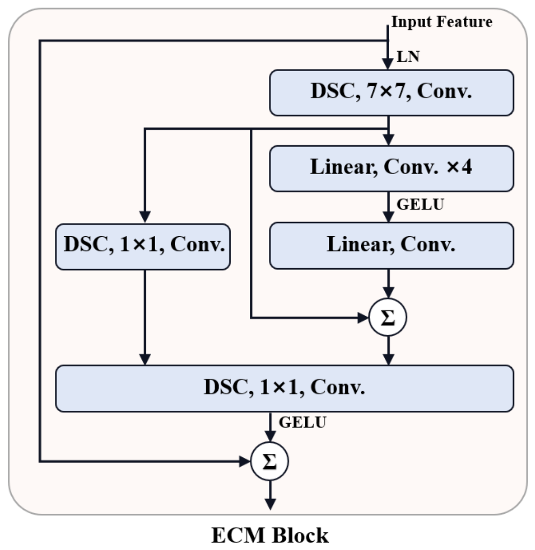
Infrared small-target detection requires sufficient local contextual information to distinguish weak target responses from surrounding structured clutter. Enlarging the local observation range is therefore beneficial, while directly increasing the spatial kernel size of standard convolution may introduce additional parameters and computational overhead. In ECM, we employ a 7 × 7 depthwise convolution followed by pointwise channel projection to provide broader local contextual modeling at relatively low computational cost. The emphasis of ECM is not on the kernel size itself, but on efficiently incorporating broader local context into a residual feature-transformation block for weak-target preservation. Its structure is shown in Figure 2.

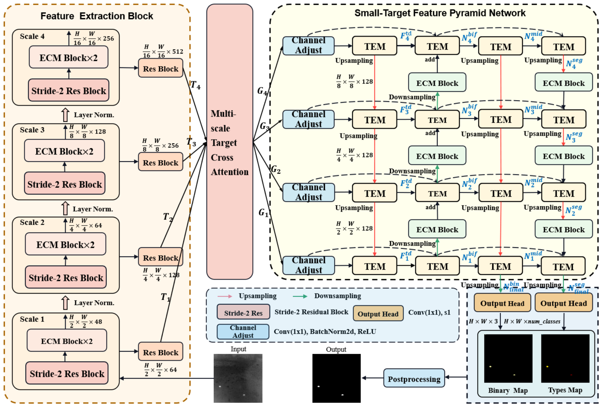
As shown in Figure 1, the encoder of PTPN consists of four consecutive stages. Each stage first reduces the spatial resolution through a stride-2 residual downsampling block (Stride-2 Res Block), followed by two cascaded ECM blocks for feature extraction. The four stages produce encoded features $T_i\left(i=1,2,3,4\right)$, with spatial resolutions of $H/2\times W/2$, $H/4\times W/4$, $H/8\times W/8$, and $H/16\times W/16$, respectively. These features are subsequently fed into the MTCA module. The following describes the forward propagation of a single ECM block. For simplicity, the batch dimension is omitted, and the input feature of the module is denoted by $x_0\in {\mathbb{R}}^{H^{\prime }\times W^{\prime }\times C}$, where $H^{\prime }$, $W^{\prime }$, and $C$ represent the feature height, width, and channel number of the current encoding stage, respectively, and $C$ corresponds to the feature channel number $C_i$ of the $i$-th encoding stage defined above. When the generic notation $H^{\prime }$, $W^{\prime }$, and $C$ are used to describe an operation within the $i$-th encoder stage, it corresponds to the stage-specific dimensions $H_i$, $W_i$, and $C_i$, respectively; i.e., $H^{\prime }=H_i$, $W^{\prime }=W_i$, and $C=C_i$.

First, ECM applies layer normalization to the input feature $x_0$ and extracts contextual information over an enlarged local spatial neighborhood through a $7\times 7$ depthwise separable convolution. The convolution output is fused with the original input via a residual connection to obtain enhanced contextual features $x_1$:

$$x_1=x_0+{\mathrm{D}\mathrm{S}\mathrm{C}\mathrm{o}\mathrm{n}\mathrm{v}}_{7\times 7}^{C\to C}\left(\mathrm{L}\mathrm{N}\left(x_0\right)\right),\hspace{1em}{x}_1\in {\mathbb{R}}^{H^{\prime }\times W^{\prime }\times C}$$

(4)

where $\mathrm{L}\mathrm{N}\left(·\right)$ denotes layer normalization, and ${\mathrm{D}\mathrm{S}\mathrm{C}\mathrm{o}\mathrm{n}\mathrm{v}}_{7\times 7}^{C\to C}\left(·\right)$ denotes a depthwise separable convolution composed of a $7\times 7$ depthwise convolution followed by a $1\times 1$ pointwise convolution. The residual connection keeps the input response available for subsequent feature transformation.

Subsequently, the contextual feature is fed into two parallel feature transformation branches. The main branch expands the channel dimension from $C$ to $4C$ through linear projection to increase the representational capacity for subsequent nonlinear transformation. The auxiliary branch first performs channel-wise transformation using a $1\times 1$ depthwise separable convolution and then maps features from $C$ to $4C$ via up-projection, providing a lightweight complementary transformation path for the main branch:

$$x_{\mathrm{e}}={\mathrm{L}\mathrm{i}\mathrm{n}\mathrm{e}\mathrm{a}\mathrm{r}}_{C\to 4C}\left(x_1\right),x_{\mathrm{r}}={\mathrm{D}\mathrm{S}\mathrm{C}\mathrm{o}\mathrm{n}\mathrm{v}}_{1\times 1}^{C\to 4C}\left(x_1\right),x_{\mathrm{e}},x_{\mathrm{r}}\in {\mathbb{R}}^{H^{\prime }\times W^{\prime }\times 4C}$$

(5)

where ${\mathrm{L}\mathrm{i}\mathrm{n}\mathrm{e}\mathrm{a}\mathrm{r}}_{C\to 4C}$ denotes linear channel projection implemented by a $1\times 1$ convolution, and ${\mathrm{D}\mathrm{S}\mathrm{C}\mathrm{o}\mathrm{n}\mathrm{v}}_{1\times 1}^{\mathrm{C}\to 4\mathrm{C}}\left(·\right)$ denotes a lightweight channel transformation composed of a $\left(1\times 1\right)$ depthwise separable convolution. Both branches maintain identical spatial resolution and output dimensionality, enabling subsequent element-wise fusion.

After obtaining the two-branch features, ECM applies GELU non-linear activation to the main branch output and adds it to the auxiliary branch output. The fused representation is then projected back to the original channel dimension (C) through a linear mapping:

$$x_2={\mathrm{L}\mathrm{i}\mathrm{n}\mathrm{e}\mathrm{a}\mathrm{r}}_{4C\to C}\left(\mathrm{G}\mathrm{E}\mathrm{L}\mathrm{U}\left(x_e\right)+x_r\right),\hspace{1em}{x}_2\in {\mathbb{R}}^{H^{\prime }\times W^{\prime }\times C}$$

(6)

where $\mathrm{G}\mathrm{E}\mathrm{L}\mathrm{U}\left(\cdot \right)$ denotes the Gaussian Error Linear Unit activation function. The channel expansion and nonlinear transformation enhance feature expressiveness, while the auxiliary branch provides an additional lightweight transformation path that reduces information loss caused by a single transformation stream. Finally, channel compression restores dimensional consistency with the input, ensuring stable feature propagation within the module.

Finally, ECM applies a GELU activation followed by a $\left(1\times 1\right)$ depthwise separable channel transformation to the compressed feature $x_2$. The transformed feature is then fused with the contextual feature $x_1$ through a second residual connection to produce the module output $x_{\mathrm{o}\mathrm{u}\mathrm{t}}$:

$$x_{\mathrm{o}\mathrm{u}\mathrm{t}}=x_1+{\mathrm{D}\mathrm{S}\mathrm{C}\mathrm{o}\mathrm{n}\mathrm{v}}_{1\times 1}^{C\to C}\left(\mathrm{G}\mathrm{E}\mathrm{L}\mathrm{U}\left(x_2\right)\right),\hspace{1em}{x}_{\mathrm{o}\mathrm{u}\mathrm{t}}\in {\mathbb{R}}^{H^{\prime }\times W^{\prime }\times C}$$

(7)

This residual connection reintegrates the transformed features obtained through channel expansion, fusion, and compression into the contextual representation, helping preserve the target–background relationships extracted in the preceding stage while facilitating gradient propagation. Since $x_{\mathrm{o}\mathrm{u}\mathrm{t}}$ has the same spatial resolution and channel dimension as $x_0$, multiple ECM blocks can be stacked sequentially within the same encoding stage without requiring additional feature alignment operations.

From the perspective of computational efficiency, for a standard $7\times 7$ convolution with both input and output channel numbers equal to $C$, the number of parameters is $49C^2$ (excluding the bias term), and the computational complexity is proportional to $H^{\prime }{W}^{\prime }\times 49C^2$. In contrast, the $7\times 7$ depthwise separable convolution in Equation (4) consists of a depthwise convolution with $49C$ parameters and a pointwise convolution with $C^2$ parameters, resulting in a total of $49C+C^2$ parameters and a computational complexity proportional to $H^{\prime }{W}^{\prime }\left(49C+C^2\right)$. Compared with a standard convolution using the same spatial kernel size, this depthwise-separable implementation substantially reduces the parameter count and computational overhead, making broader-context convolutional operators more practical for repeated deployment across multiple encoder stages. It should be noted that the above comparison considers only the $7\times 7$ convolutional operator in ECM and excludes the additional overhead introduced by channel expansion, linear projection, and the auxiliary branch.

Overall, ECM follows a context extraction-complementary transformation-residual refinement pipeline. The block is not intended to simply replace a standard convolution with a cheaper operator; rather, it enlarges the local observation range while preserving the response path of small targets. Therefore, the encoded multi-scale features contain both contextual separability and fine spatial evidence, which are required by the subsequent MTCA module.

3.3. MTCA

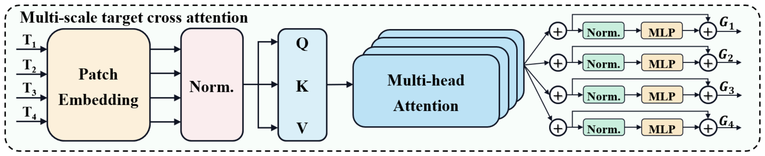
Conventional FPN-like structures usually exchange information between adjacent scales through addition or concatenation. Such fixed fusion may not be sufficient for small infrared targets, because shallow layers contain location-sensitive but noisy responses, whereas deep layers contain stronger semantics but weaker spatial detail. To enable more selective cross-scale communication, we introduce the Multi-scale Target Cross-Attention (MTCA) module, as illustrated in Figure 3.

MTCA receives four-level features generated by the ECM encoder, denoted as $\mathcal{T}=\left\{T_1,T_2,T_3,T_4\right\}$, where $T_i\in {\mathbb{R}}^{H_i\times W_i\times C_i}$, and $H_i$, $W_i$, and $C_i$ denote the height, width, and channel dimension of the $i$-th stage feature, respectively. The spatial dimensions satisfy $H_i=H/2^i$ and $W_i=W/2^i$ for $i=1,2,3,4$. Since features at different scales differ in both spatial resolution and channel dimension, directly flattening them into token sequences would produce much longer sequences for high-resolution features, which not only substantially increases the computational cost of cross-scale attention but also leads to imbalanced computation among different scales. To overcome this issue, MTCA first constructs multi-scale token representations with unified quantity and embedding dimension through scale-adaptive patch embedding. Cross-scale information retrieval and feature reconstruction are then performed at a unified token granularity. Specifically, the module consists of three stages: scale-aligned token embedding, asymmetric cross-scale attention, and feed-forward refinement with feature restoration.

For the $i$-th scale, MTCA partitions the feature map $T_i$ into non-overlapping patches with side length $p_i$, and projects each patch into a $D$-dimensional token space through a scale-specific embedding function ${\mathcal{E}}_i\left(\cdot \right)$. The patch sizes for the four scales are set to $\left(\left(p_1,p_2,p_3,p_4\right)=\left(16,8,4,2\right)\right)$, respectively. After scale-adaptive patch embedding, the stage-specific spatial dimensions $\left(H_i,W_i\right)$ are mapped to the unified dimensions $\left(H^{\prime },W^{\prime }\right)$, where $H^{\prime }=H_i/p_i$ and $W^{\prime }=W_i/p_i$. Meanwhile, the stage-specific channel dimension $C_i$ is projected to the common embedding dimension $C=D$; therefore, each scale produces $N=H^{\prime }{W}^{\prime }$ tokens with the same embedding dimension. The corresponding token $E_i$ representation is given by:

$$E_i={\mathcal{E}}_i\left(T_i\right)\in {\mathbb{R}}^{N\times D},\hspace{1em}N=H^{\prime }{W}^{\prime }={\displaystyle \frac{H_i{W}_i}{p_i^2}}={\displaystyle \frac{HW}{1024}},\hspace{1em}i=1,2,3,4$$

(8)

where ${\mathcal{E}}_i\left(\cdot \right)$ denotes the scale-specific patch embedding operation. We assume that the height and width of the input image are divisible by 32, which can be readily satisfied in practice through zero padding when necessary. Since the feature resolution and patch size decrease proportionally across the four scales, $H^{\prime }$, $W^{\prime }$, and $N$ are identical for all four feature levels, while their original stage-specific channel dimensions $C_i$ are projected to the common embedding dimension $D$. From a geometric perspective, the tokens at different scales each correspond to approximately a $\left(32\times 32\right)$ region in the input image, enabling direct comparison of multi-scale features at a consistent spatial granularity. It should be noted that this region only represents the geometric coverage of each patch in the input coordinate space rather than the actual receptive field of the network features. Fine-grained localization information is still preserved by the residual connections in the encoder and the subsequent STFPN.

After obtaining the scale-aligned token representations, MTCA applies layer normalization to each scale and concatenates tokens along the token dimension to form a global multi-scale context sequence. Unlike standard self-attention that treats all tokens as a single sequence, MTCA preserves scale-specific queries while constructing shared keys and values from the concatenated multi-scale sequence. Let the multi-head attention contain $\left(h\right)$ heads, with each head dimension $d=D/h$. Then, for the $i$-th scale and the $\left(j\right)$-th attention head, the queries, keys, and values are formulated as:

$${\overline{E}}_i=\mathrm{L}\mathrm{N}\left(E_i\right),\overline{E}=\mathrm{C}\mathrm{o}\mathrm{n}\mathrm{c}\mathrm{a}\mathrm{t}\left({\overline{E}}_1,{\overline{E}}_2,{\overline{E}}_3,{\overline{E}}_4\right),Q_{i,j}={\overline{E}}_i{W}_{i,j}^Q,\hspace{1em}{K}_j=\overline{E}{W}_j^K,\hspace{1em}{V}_j=\overline{E}{W}_j^V$$

(9)

where $\overline{E}\in {\mathbb{R}}^{4N\times D}$, $Q_{i,j}\in {\mathbb{R}}^{N\times d}$, and $K_j,V_j\in {\mathbb{R}}^{4N\times d}$. $W_{i,j}^Q\in {\mathbb{R}}^{D\times d}$ denotes the scale-specific query projection matrix, while $W_j^K,W_j^V\in {\mathbb{R}}^{D\times d}$ are shared key and value projection matrices across different scales. The scale-specific query design allows each level to formulate distinct information retrieval requirements according to its feature distribution, while the shared key–value sequence provides candidate contextual information from all scales.

For the $j$-th attention head, cross-scale relevance is first computed between the current-scale queries and the global key sequence, followed by weighted aggregation over the value sequence. The outputs of all attention heads are concatenated and linearly projected to obtain the cross-scale attention representation of the $i$-th scale:

$$H_{i,j}=\mathrm{S}\mathrm{o}\mathrm{f}\mathrm{t}\mathrm{m}\mathrm{a}\mathrm{x}\left({\displaystyle \frac{Q_{i,j}{K}_j^T}{\sqrt{d}}}\right)V_j,A_i=\mathrm{C}\mathrm{o}\mathrm{n}\mathrm{c}\mathrm{a}\mathrm{t}\left(H_{i,1},H_{i,2},\dots ,H_{i,h}\right)W^O$$

(10)

where $H_{i,j}\in {\mathbb{R}}^{N\times d}$, $A_i\in {\mathbb{R}}^{N\times D}$, and $W^O\in {\mathbb{R}}^{D\times D}$ is the output projection matrix. In this work, the number of attention heads is set to $h=2$. No explicit absolute or relative positional encoding is employed in MTCA. Instead, spatial correspondence across different scales is established during the preceding scale-adaptive patch embedding. Since the feature resolutions and patch sizes decrease proportionally across the four scales, all feature levels are mapped to token grids with identical spatial dimensions and the same number of tokens $N$. Therefore, cross-scale attention is performed at a unified spatial granularity, with the attention weights determined by feature-content similarity.

Through this asymmetric query–global key design, each scale updates its own token representation while selectively retrieving complementary information from all scales. Shallow queries can access deeper contextual semantics to reduce background clutter, while deep queries can leverage fine-grained spatial cues from shallow features, thereby improving cross-scale consistency and preserving weak target responses in complex scenes.

The cross-scale attention output is first fused with the original token representation of the corresponding scale through a residual connection, followed by layer normalization to stabilize feature distributions. A scale-specific feed-forward network is then employed to further perform nonlinear feature transformation:

$$U_i=\mathrm{L}\mathrm{N}\left(E_i+A_i\right),{\tilde{E}}_i=U_i+{\mathrm{F}\mathrm{F}\mathrm{N}}_i\left(U_i\right),\hspace{1em}{\tilde{E}}_i\in {\mathbb{R}}^{N\times D}$$

(11)

The ${\mathrm{F}\mathrm{F}\mathrm{N}}_i\left(·\right)$ adopts a bottleneck architecture consisting of channel expansion, local token transformation, and channel compression:

$${\mathrm{F}\mathrm{F}\mathrm{N}}_i\left(Z\right)={\mathcal{P}}_{rD\to D}\left(\sigma \right({\mathcal{D}}_{\mathrm{t}\mathrm{o}\mathrm{k}}^i\left({\mathcal{P}}_{D\to rD}\left(Z\right)\right)$$

(12)

where ${\mathcal{P}}_{D\to rD}\left(\cdot \right)$ and ${\mathcal{P}}_{rD\to D}\left(\cdot \right)$ denote channel expansion and channel compression, respectively, $\left(r\right)$ is the channel expansion ratio, and $\sigma \left(\cdot \right)$ denotes the GELU activation function. ${\mathcal{D}}_{\mathrm{t}\mathrm{o}\mathrm{k}}^i\left(\cdot \right)$ reshapes the token sequence into a two-dimensional feature map, performs depthwise convolution, and then flattens it back into a token sequence, thereby introducing local spatial inductive bias to complement the cross-scale interaction performed by the attention module. Independent feed-forward network parameters are adopted for different scales to better accommodate their distinct feature distributions.

Finally, MTCA restores the cross-scale enhanced tokens to two-dimensional feature maps of the corresponding resolutions through the scale-specific inverse patch embedding function ${\mathcal{R}}_i\left(\cdot \right)$. Specifically, each token is first projected into a patch representation with dimension $p_i^2{C}_i$, followed by a Fold operation for spatial reconstruction. The reconstructed feature is then fused with the original encoder feature through a residual connection:

$$G_i=T_i+{\mathcal{R}}_i\left({\tilde{E}}_i\right),\hspace{1em}{\mathcal{R}}_i\left({\tilde{E}}_i\right)={\mathrm{F}\mathrm{o}\mathrm{l}\mathrm{d}}_{p_i}\left({\mathcal{P}}_{D\to p_i^2{C}_i}\left({\tilde{E}}_i\right)\right),\hspace{1em}{G}_i\in {\mathbb{R}}^{H_i\times W_i\times C_i}$$

(13)

The reconstruction branch injects cross-scale contextual information into the original encoded features, while the residual connection with $T_i$ preserves the intrinsic spatial responses of the current scale. Consequently, MTCA transforms the encoded feature set $\left(\mathcal{T}\right)$ into the cross-scale enhanced feature set $\mathcal{G}=G_1,G_2,G_3,G_4$, while maintaining the original spatial resolutions and channel configurations of the four-level feature pyramid, enabling seamless input to the subsequent STFPN.

For each scale, the query sequence contains N tokens, whereas the global key–value sequence contains 4N tokens. Therefore, the dominant computational complexity of single-scale attention is $O\left(4N^{2}D\right)$, and the total complexity over the four scales is $O\left(16N^{2}D\right)$. This asymptotic complexity is equivalent to that of applying a single global self-attention operation over 4N tokens. Hence, the primary objective of the asymmetric query–key architecture is not to reduce the theoretical quadratic complexity under the same token budget but to preserve independent information retrieval and feature update pathways for each scale. In practice, the computational cost of MTCA is mainly controlled by the scale-adaptive patch embedding, which compresses the token sequence length of high-resolution features. Additional computation arises from the query, key, value, output projection, and feed-forward network operations.

Overall, MTCA enables scale-specific retrieval of complementary information from the shared multi-scale context while preserving the hierarchical feature structure, providing cross-scale enhanced representations for the subsequent STFPN.

3.4. STFPN

Although MTCA enhances cross-scale interaction, weak targets may still be suppressed during hierarchical propagation. To further strengthen target responses, a Small-Target Feature Pyramid Network (STFPN) is designed.

Given the cross-scale enhanced feature set produced by MTCA $\mathcal{G}=G_1,G_2,G_3,G_4$, where $G_i\in {\mathbb{R}}^{H_i\times W_i\times C_i}$, STFPN first projects features at different scales into a unified channel dimension $C_f=128$ through a channel adjustment module and then introduces a Target Enhancement Module (TEM) to strengthen weak target responses at each scale, yielding the initial target-enhanced pyramid features:

$$A_i={\mathcal{C}}_i\left(G_i\right),P_i^{\mathrm{m}\mathrm{i}\mathrm{d}}=\mathrm{T}\mathrm{E}\mathrm{M}\left(A_i\right),A_i,P_i^{\mathrm{m}\mathrm{i}\mathrm{d}}\in {\mathbb{R}}^{H_i\times W_i\times C_f},i=1,2,3,4,$$

(14)

where $C_i\left(\cdot \right)$ denotes the channel adjustment operation consisting of a $1\times 1$ convolution, batch normalization, and ReLU activation. $P_i^{\mathrm{m}\mathrm{i}\mathrm{d}}$ represents the initial target-enhanced pyramid feature before entering the bidirectional fusion pathways. Through this step, features from different scales are first projected into a common channel space, while preliminary enhancement of weak target responses is performed before cross-scale propagation.

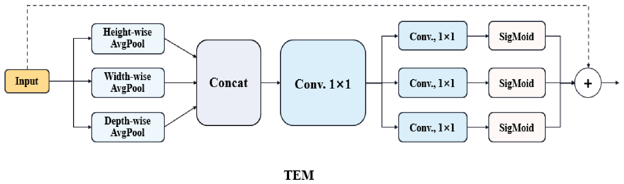
TEM serves as the fundamental enhancement unit in STFPN, and its architecture is illustrated in Figure 4. Given an input feature map $X\in {\mathbb{R}}^{H^{\prime }\times W^{\prime }\times C_f}$, TEM extracts statistical descriptors along the height, width, and channel dimensions to generate direction-aware attention weights. Specifically, TEM performs average pooling along the width dimension while preserving the height dimension to obtain the height descriptor $z^h\in {\mathbb{R}}^{H^{\prime }\times 1\times C_f}$; average pooling along the height dimension while preserving the width dimension to obtain the width descriptor $z^w\in {\mathbb{R}}^{1\times W^{\prime }\times C_f}$; and global average pooling over both spatial dimensions to obtain the channel descriptor $z^c\in {\mathbb{R}}^{1\times 1\times C_f}$:

$$z^h={\mathrm{A}\mathrm{v}\mathrm{g}\mathrm{P}\mathrm{o}\mathrm{o}\mathrm{l}}_w\left(X\right),z^w={\mathrm{A}\mathrm{v}\mathrm{g}\mathrm{P}\mathrm{o}\mathrm{o}\mathrm{l}}_h\left(X\right),z^c={\mathrm{A}\mathrm{v}\mathrm{g}\mathrm{P}\mathrm{o}\mathrm{o}\mathrm{l}}_{h,w}\left(X\right)$$

(15)

where ${\mathrm{A}\mathrm{v}\mathrm{g}\mathrm{P}\mathrm{o}\mathrm{o}\mathrm{l}}_w\left(\cdot \right)$ denotes average pooling along the width dimension, ${\mathrm{A}\mathrm{v}\mathrm{g}\mathrm{P}\mathrm{o}\mathrm{o}\mathrm{l}}_h\left(\cdot \right)$ denotes average pooling along the height dimension, and ${\mathrm{A}\mathrm{v}\mathrm{g}\mathrm{P}\mathrm{o}\mathrm{o}\mathrm{l}}_h\left(\cdot \right)$ denotes global average pooling over both spatial dimensions.

Since $z^h$, $z^w$, and $z^c$ have different spatial shapes, TEM first transforms the width descriptor into the same coordinate sequence format as the height descriptor before concatenation, while treating the channel descriptor as a global coordinate token with sequence length one. The three descriptors are then concatenated along the coordinate dimension and passed through a shared feature transformation, after which they are split back into three direction-specific intermediate representations:

$$S={\mathrm{C}\mathrm{o}\mathrm{n}\mathrm{c}\mathrm{a}\mathrm{t}}_s(z^h,\mathrm{P}\mathrm{e}\mathrm{r}\mathrm{m}\mathrm{u}\mathrm{t}\mathrm{e}(z^w),z^c),[u^h,u^w,u^c]={\mathrm{S}\mathrm{p}\mathrm{l}\mathrm{i}\mathrm{t}}_s\left(\varphi \right({\mathrm{C}\mathrm{o}\mathrm{n}\mathrm{v}}_{1\times 1}\left(S\right))$$

(16)

where $\mathrm{P}\mathrm{e}\mathrm{r}\mathrm{m}\mathrm{u}\mathrm{t}\mathrm{e}\left(\cdot \right)$ transforms $z^w\in {\mathbb{R}}^{1\times W^{\prime }\times C_f}$ into ${\mathbb{R}}^{W^{\prime }\times 1\times C_f}$, the concatenated feature $S\in {\mathbb{R}}^{(H^{\prime }+W^{\prime }+1)\times 1\times C_f}$, ${\mathrm{C}\mathrm{o}\mathrm{n}\mathrm{c}\mathrm{a}\mathrm{t}}_{\mathrm{s}}\left(\cdot \right)$ denotes concatenation along the coordinate dimension; ${\mathrm{S}\mathrm{p}\mathrm{l}\mathrm{i}\mathrm{t}}_s\left(\cdot \right)$ splits the sequence according to lengths $H^{\prime }$, $W^{\prime }$, and 1, respectively; and $\varphi \left(\cdot \right)$ denotes the nonlinear activation function. After splitting, $u^h\in {\mathbb{R}}^{H^{\prime }\times 1\times C_f}$, $u^w\in {\mathbb{R}}^{W^{\prime }\times 1\times C_f}$, and $u^c\in {\mathbb{R}}^{1\times 1\times C_f}$.

Subsequently, the three intermediate representations are independently projected and activated by the Sigmoid function to generate attention weights along the height, width, and channel directions:

$${\alpha }^h=\mathrm{S}\mathrm{i}\mathrm{g}\mathrm{m}\mathrm{o}\mathrm{i}\mathrm{d}\left({\mathcal{F}}_h\left(u^h\right)\right),{\alpha }^w={\mathrm{P}\mathrm{e}\mathrm{r}\mathrm{m}\mathrm{u}\mathrm{t}\mathrm{e}}^{-1}\left[\mathrm{S}\mathrm{i}\mathrm{g}\mathrm{m}\mathrm{o}\mathrm{i}\mathrm{d}\right({\mathcal{F}}_w\left(u^w\right)\left)\right],{\alpha }^c=\mathrm{S}\mathrm{i}\mathrm{g}\mathrm{m}\mathrm{o}\mathrm{i}\mathrm{d}\left({\mathcal{F}}_c\left(u^c\right)\right)$$

(17)

where ${\mathcal{F}}_h\left(\cdot \right)$, ${\mathcal{F}}_w\left(\cdot \right)$, and ${\mathcal{F}}_c\left(\cdot \right)$ denote direction-specific linear mappings. ${\mathrm{P}\mathrm{e}\mathrm{r}\mathrm{m}\mathrm{u}\mathrm{t}\mathrm{e}}^{-1}\left(\cdot \right)$ restores the width-direction attention to the shape ${\mathbb{R}}^{1\times W^{\prime }\times C_f}$. Consequently, ${\alpha }^h\in {\mathbb{R}}^{H^{\prime }\times 1\times C_f}$, ${\alpha }^w\in {\mathbb{R}}^{1\times W^{\prime }\times C_f}$, and ${\alpha }^c\in {\mathbb{R}}^{1\times 1\times C_f}$. These three attention maps are multiplied with the input feature through broadcasting to obtain the output of TEM:

$$\mathrm{T}\mathrm{E}\mathrm{M}\left(X\right)=X\odot {\alpha }^h\odot {\alpha }^w\odot {\alpha }^c$$

(18)

where $\odot$ denotes element-wise multiplication. Compared with attention mechanisms that model only channel statistics, TEM simultaneously preserves statistical information along both the height and width directions, enabling it to enhance weak target responses while effectively suppressing background responses aggregated along specific spatial directions.

After obtaining the initial target-enhanced pyramid features $P_i^{\mathrm{m}\mathrm{i}\mathrm{d}}$, STFPN constructs a bidirectional fusion architecture to facilitate interaction between deep contextual semantics and shallow spatial details. First, a top-down pathway is built from the deepest level, progressively upsampling low-resolution semantic features to higher-resolution layers and fusing them with the target-enhanced features at the corresponding scales:

$$F_4^{\mathrm{t}\mathrm{d}}=\mathrm{T}\mathrm{E}\mathrm{M}\left(P_4^{\mathrm{m}\mathrm{i}\mathrm{d}}\right),\hspace{1em}{F}_i^{\mathrm{t}\mathrm{d}}=\mathrm{T}\mathrm{E}\mathrm{M}\left(P_i^{\mathrm{m}\mathrm{i}\mathrm{d}}\right)+\mathrm{U}\mathrm{p}\left(F_{i+1}^{\mathrm{t}\mathrm{d}}\right),\hspace{1em}i=3,2,1,$$

(19)

where $\mathrm{U}\mathrm{p}\left(\cdot \right)$ denotes the upsampling operation that adjusts the feature map at the $\left(i+1\right)$-th level to the spatial resolution of the $i$-th level. $F_i^{\mathrm{t}\mathrm{d}}$ represents the fused feature generated by the top-down pathway. This pathway propagates large-scale contextual information from deeper layers to shallower layers, thereby improving the separability between small targets and complex backgrounds.

Subsequently, STFPN constructs a bottom-up detail feedback pathway to progressively propagate high-resolution spatial details into deeper semantic features, compensating for the small-target localization cues that may be lost during top-down propagation:

$$N_1^{\mathrm{b}\mathrm{i}\mathrm{f}}=\mathrm{T}\mathrm{E}\mathrm{M}\left(F_1^{\mathrm{t}\mathrm{d}}\right),\hspace{1em}{N}_i^{\mathrm{b}\mathrm{i}\mathrm{f}}=\mathrm{T}\mathrm{E}\mathrm{M}\left(F_i^{\mathrm{t}\mathrm{d}}\right)+\mathrm{D}\mathrm{o}\mathrm{w}\mathrm{n}\left(N_{i-1}^{\mathrm{b}\mathrm{i}\mathrm{f}}\right),\hspace{1em}i=2,3,4$$

(20)

where $\mathrm{D}\mathrm{o}\mathrm{w}\mathrm{n}\left(\cdot \right)$ denotes the downsampling operation for matching the spatial resolutions between adjacent feature levels. $N_i^{\mathrm{b}\mathrm{i}\mathrm{f}}$ denotes the bidirectionally fused feature generated by the bottom-up pathway. Through this pathway, the rich spatial localization cues preserved in shallow layers are progressively fed back into deeper semantic representations, enabling weak target responses to maintain stronger localization consistency across different scales.

To further obtain high-resolution features suitable for pixel-wise prediction, STFPN constructs a segmentation refinement branch based on $N_i^{\mathrm{b}\mathrm{i}\mathrm{f}}$. Since the bottom-up pathway has already aggregated fine-grained spatial details into deeper features, the segmentation refinement branch starts from the deepest bidirectionally fused feature and performs another top-down propagation, allowing deep semantic information to be realigned with high-resolution responses before prediction:

$$N_4^{\mathrm{s}\mathrm{e}\mathrm{g}}=\mathrm{T}\mathrm{E}\mathrm{M}\left(N_4^{\mathrm{b}\mathrm{i}\mathrm{f}}\right),N_i^{\mathrm{s}\mathrm{e}\mathrm{g}}=\mathrm{T}\mathrm{E}\mathrm{M}\left(N_i^{\mathrm{b}\mathrm{i}\mathrm{f}}\right)+\mathrm{U}\mathrm{p}\left(N_{i+1}^{\mathrm{s}\mathrm{e}\mathrm{g}}\right),i=3,2,1$$

(21)

where $N_i^{\mathrm{s}\mathrm{e}\mathrm{g}}$ denotes the output feature of the segmentation refinement branch at the $i$-th scale. This branch further propagates deep contextual information to the highest-resolution feature maps while further enhancing local details and target localization responses prior to the final pixel-wise prediction.

Finally, STFPN feeds the highest-resolution bidirectionally fused feature $N_1^{\mathrm{b}\mathrm{i}\mathrm{f}}$ and the segmentation refinement feature $N_1^{\mathrm{s}\mathrm{e}\mathrm{g}}$ into two lightweight prediction heads to generate the foreground/background binary classification logits for the two branches:

$$Z^{\mathrm{b}\mathrm{i}\mathrm{f}}={\mathcal{H}}_{\mathrm{b}\mathrm{i}\mathrm{f}}\left(N_1^{\mathrm{b}\mathrm{i}\mathrm{f}}\right),\hspace{1em}{Z}^{\mathrm{s}\mathrm{e}\mathrm{g}}={\mathcal{H}}_{\mathrm{s}\mathrm{e}\mathrm{g}}\left(N_1^{\mathrm{s}\mathrm{e}\mathrm{g}}\right),\hspace{1em}{Z}^{\mathrm{b}\mathrm{i}\mathrm{f}},Z^{\mathrm{s}\mathrm{e}\mathrm{g}}\in {\mathbb{R}}^{H^{\prime }\times W^{\prime }\times 2}$$

(22)

where ${\mathcal{H}}_{\mathrm{b}\mathrm{i}\mathrm{f}}\left(\cdot \right)$ and ${\mathcal{H}}_{\mathrm{s}\mathrm{e}\mathrm{g}}\left(\cdot \right)$ are lightweight prediction heads consisting of a $1\times 1$ convolution followed by an upsampling operation. Both branches perform pixel-wise foreground/background binary classification rather than additional target category prediction. The bidirectional fusion branch $Z^{\mathrm{b}\mathrm{i}\mathrm{f}}$ primarily exploits the multi-scale contextual information aggregated by the bidirectional fusion pathway, whereas the segmentation refinement branch $Z^{\mathrm{s}\mathrm{e}\mathrm{g}}$ further enhances high-resolution spatial details through the refinement pathway. During training, both prediction branches are jointly supervised. During inference, the foreground probabilities from the two branches are fused according to Equation (2) to obtain the final detection probability map.

In summary, STFPN converts the MTCA-enhanced feature set into target-preserving prediction features through channel alignment, TEM-based response enhancement, top-down semantic propagation, bottom-up detail feedback, and segmentation refinement. Compared with a standard pyramid decoder, STFPN emphasizes weak-target responses before and during feature propagation, which helps reduce missed detections caused by repeated downsampling and multi-level fusion.

From an interaction perspective, ECM, MTCA, and STFPN operate sequentially and complementarily. ECM provides context-enriched multi-level representations, MTCA selectively retrieves complementary information from the shared multi-scale context, and STFPN further aggregates and propagates the interacted features through bidirectional pyramid fusion and refinement. Together, they form a progressive context modeling–cross-scale interaction–target-preserving aggregation pathway that preserves weak target responses while integrating semantic and localization information across scales.

3.5. PCL

Conventional data-driven loss functions mainly constrain the consistency between prediction results and pixel-wise annotations but do not explicitly exploit the physical characteristics of small infrared target imaging. Under conditions of low signal-to-noise ratio, complex background clutter, or local high-intensity interference, the network may produce false responses that are inconsistent with infrared imaging characteristics. To address this issue, this paper proposes a Physics-Constrained Loss (PCL), which regularizes the prediction from three complementary perspectives: point spread function consistency, relative intensity consistency within target regions, and signal-to-noise-ratio-aware constraints. PCL serves as a physics-inspired regularization term in addition to the conventional data-driven supervision. It should be noted that PCL is involved only during training and does not modify the network architecture or computational pipeline during inference.

According to the dual-branch prediction mechanism described in Section 3.1, PTPN outputs foreground probability maps from the bidirectional-fusion branch and the segmentation-refinement branch, denoted by ${\widehat{Y}}^r$, where $r\in \mathrm{b}\mathrm{i}\mathrm{f},\mathrm{s}\mathrm{e}\mathrm{g}$. This notation is a simplified form of ${\widehat{Y}}^{\mathrm{b}\mathrm{i}\mathrm{f}}$ and ${\widehat{Y}}^{\mathrm{s}\mathrm{e}\mathrm{g}}$ introduced in Section 3.1. Given the binary ground-truth mask $Y\in {0,1}^{H\times W}$ and the normalized infrared intensity image $I\in {\left[0,1\right]}^{H\times W}$, both branches are supervised by the data-driven loss and the physics-constrained loss. The overall training objective is defined as:

$$\begin{array}{c} {\mathcal{L}}_{\mathrm{t}\mathrm{o}\mathrm{t}\mathrm{a}\mathrm{l}}={\displaystyle \sum _{r\in \left\{\mathrm{b}\mathrm{i}\mathrm{f},\mathrm{s}\mathrm{e}\mathrm{g}\right\}}}\left({\mathcal{L}}_{\mathrm{d}\mathrm{a}\mathrm{t}\mathrm{a}}^r+{\lambda }_{\mathrm{p}\mathrm{c}\mathrm{l}}{\mathcal{L}}_{\mathrm{p}\mathrm{c}\mathrm{l}}^r\right) \end{array}$$

(23)

where ${\mathcal{L}}_{\mathrm{d}\mathrm{a}\mathrm{t}\mathrm{a}}^r$ denotes the data-driven loss for the $\mathrm{r}$-th prediction branch, ${\mathcal{L}}_{\mathrm{p}\mathrm{c}\mathrm{l}}^{\mathrm{r}}$ denotes the corresponding physics-constrained loss, and ${\lambda }_{\mathrm{p}\mathrm{c}\mathrm{l}}$ is the weighting coefficient of PCL. For simplicity, the following derivations use the foreground probability map $\widehat{Y}$ from a single prediction branch as an example, while the actual training loss is obtained by summing the losses of both branches.

The data-driven supervision consists of the Focal Loss and the Soft $IoU$ Loss, jointly constraining pixel-wise foreground/background classification accuracy and target localization quality:

$${\mathcal{L}}_{\mathrm{d}\mathrm{a}\mathrm{t}\mathrm{a}}={\lambda }_{\mathrm{f}\mathrm{o}\mathrm{c}\mathrm{a}\mathrm{l}}{\mathcal{L}}_{\mathrm{f}\mathrm{o}\mathrm{c}\mathrm{a}\mathrm{l}}+{\lambda }_{\mathrm{i}\mathrm{o}\mathrm{u}}{\mathcal{L}}_{\mathrm{i}\mathrm{o}\mathrm{u}}$$

(24)

where ${\lambda }_{\mathrm{f}\mathrm{o}\mathrm{c}\mathrm{a}\mathrm{l}}$ and ${\lambda }_{\mathrm{i}\mathrm{o}\mathrm{u}}$ denote the weighting coefficients of the two loss terms, respectively. Since small infrared targets occupy only a tiny fraction of the image, resulting in severe foreground–background class imbalance, Focal Loss is adopted to alleviate the dominance of easy background pixels during optimization:

$${\mathcal{L}}_{\mathrm{f}\mathrm{o}\mathrm{c}\mathrm{a}\mathrm{l}}=-{\displaystyle \frac{1}{\left|\Omega \right|}}\sum _{u\in \Omega }\left[\alpha Y_u{\left(1-{\widehat{Y}}_u\right)}^{\gamma }\log \left({\widehat{Y}}_u+ϵ\right)+\left(1-\alpha \right)\left(1-Y_u\right){\widehat{Y}}_u^{\gamma }\log \left(1-{\widehat{Y}}_u+ϵ\right)\right]$$

(25)

where $\Omega$ denotes the set of image pixels, $u$ denotes the pixel index, $\alpha$ is the foreground/background balancing coefficient, $\gamma$ is the focusing parameter, and $ϵ$ is a small constant introduced to avoid numerical instability in logarithmic and division operations. The Soft $IoU$ Loss is defined as:

$${\mathcal{L}}_{\mathrm{i}\mathrm{o}\mathrm{u}}=1-{\displaystyle \frac{\sum _{u\in \Omega }{\widehat{Y}}_u{Y}_u+ϵ}{\sum _{u\in \Omega }{\widehat{Y}}_u+\sum _{u\in \Omega }{Y}_u-\sum _{u\in \Omega }{\widehat{Y}}_u{Y}_u+ϵ}}$$

(26)

which directly optimizes the overlap between the predicted region and the ground-truth target region, thereby improving the pixel-level localization quality of infrared small target detection.

The proposed PCL consists of three complementary components: a point spread function consistency loss, a target-region relative intensity consistency loss, and a signal-to-noise-ratio-aware loss:

$${\mathcal{L}}_{\mathrm{p}\mathrm{c}\mathrm{l}}={\lambda }_{\mathrm{p}\mathrm{s}\mathrm{f}}{\mathcal{L}}_{\mathrm{p}\mathrm{s}\mathrm{f}}+{\lambda }_{\mathrm{i}\mathrm{n}\mathrm{t}}{\mathcal{L}}_{\mathrm{i}\mathrm{n}\mathrm{t}}+{\lambda }_{\mathrm{s}\mathrm{n}\mathrm{r}}{\mathcal{L}}_{\mathrm{s}\mathrm{n}\mathrm{r}}$$

(27)

where ${\lambda }_{\mathrm{p}\mathrm{s}\mathrm{f}}$, ${\lambda }_{\mathrm{i}\mathrm{n}\mathrm{t}}$, and ${\lambda }_{\mathrm{s}\mathrm{n}\mathrm{r}}$ denote the weighting coefficients of the three components, respectively.

First, after passing through an optical imaging system, an infrared small target is generally not represented as an ideal isolated point but is spatially spread by the point spread function (PSF). To encourage the predicted probability map to exhibit a local response pattern consistent with the imaging process, we approximate the PSF using a normalized Gaussian kernel $K_{\sigma }$ and convolve the ground-truth mask to obtain a soft target response:

$${\tilde{Y}}_{\mathrm{p}\mathrm{s}\mathrm{f}}=\mathrm{N}\mathrm{o}\mathrm{r}\mathrm{m}\left(K\ast \sigma \ast Y\right),\hspace{1em}{\mathcal{L}}_{\mathrm{p}\mathrm{s}\mathrm{f}}={\displaystyle \frac{1}{\left|\Omega \right|}}\sum _{u\in \Omega }{\left({\widehat{Y}}_u-{\tilde{Y}}_{\mathrm{p}\mathrm{s}\mathrm{f},u}\right)}^2$$

(28)

where $\ast$ denotes the convolution operator, $\mathrm{N}\mathrm{o}\mathrm{r}\mathrm{m}\left(\cdot \right)$ normalizes the convolution result into the range $\left[0,1\right]$, and $\sigma$ controls the spatial spread of the soft target response. In practice, $\sigma$ is treated as a hyperparameter related to the typical target size and imaging blur, whose value is specified in Section 4 and analyzed in the ablation study. This loss encourages the prediction to form a smooth local spreading response within the target region while suppressing undesired scattered responses far from the target.

Second, infrared small targets are typically characterized by local radiative intensity anomalies. Strictly speaking, if reliable radiometric calibration, sensor response parameters, target temperature, and imaging wavelength are available, an absolute radiometric consistency constraint can be derived from the physical imaging model. However, commonly used infrared small target detection datasets provide only image intensities and pixel-level annotations, without such absolute physical quantities. Therefore, instead of relying on unavailable radiometric information, we adopt normalized grayscale intensity as a computable surrogate of the relative infrared response. The resulting constraint captures the physical prior that infrared small targets should exhibit local intensity anomalies, requiring the predicted foreground region to maintain a relative intensity distribution consistent with the ground-truth target region. Specifically, the weighted average intensity of the predicted foreground and the average intensity of the ground truth target are defined as:

$${\mu }_{\mathrm{p}\mathrm{r}\mathrm{e}\mathrm{d}}={\displaystyle \frac{\sum _{u\in \Omega }{\widehat{Y}}_u{I}_u}{\sum _{u\in \Omega }{\widehat{Y}}_u+ϵ}},\hspace{1em}{\mu }_{\mathrm{g}\mathrm{t}}={\displaystyle \frac{\sum _{u\in \Omega }{Y}_u{I}_u}{\sum _{u\in \Omega }{Y}_u+ϵ}}$$

(29)

and the target-region relative intensity consistency loss is formulated as:

$${\mathcal{L}}_{\mathrm{i}\mathrm{n}\mathrm{t}}={\left({\mu }_{\mathrm{p}\mathrm{r}\mathrm{e}\mathrm{d}}-{\mu }_{\mathrm{g}\mathrm{t}}\right)}^2$$

(30)

This term encourages the average infrared response within the predicted foreground region to be consistent with that of the ground-truth target region, thereby suppressing background or texture responses whose intensity distributions deviate from those of true targets. If future datasets provide reliable radiometric calibration and sensor parameters, Equation (30) can be naturally extended to a more refined absolute radiometric consistency constraint.

Finally, the reliability of infrared small target detection is closely related to the target-to-background signal-to-noise ratio (SNR). To address scenarios with common local background interference, we introduce a differentiable SNR-aware constraint that encourages the predicted foreground to correspond to regions with higher target–background separability. Since Equation (29) has already defined the weighted average intensity of the predicted foreground region as ${\mu }_{\mathrm{p}\mathrm{r}\mathrm{e}\mathrm{d}}$, we directly let:

$${\mu }_t={\mu }_{\mathrm{p}\mathrm{r}\mathrm{e}\mathrm{d}},\hspace{1em}{\mu }_b={\displaystyle \frac{\sum _{u\in \Omega }\left(1-{\widehat{Y}}_u\right)I_u}{\sum _{u\in \Omega }\left(1-{\widehat{Y}}_u\right)+ϵ}}$$

(31)

where ${\mu }_t$ and ${\mu }_b$ denote the weighted average intensities of the predicted target region and the predicted background region, respectively. The standard deviation of the background intensity is defined as:

$${\sigma }_b=\sqrt{{\displaystyle \frac{\sum _{u\in \Omega }\left(1-{\widehat{Y}}_u\right){\left(I_u-{\mu }_b\right)}^2}{\sum _{u\in \Omega }\left(1-{\widehat{Y}}_u\right)+ϵ}}+ϵ}$$

(32)

which leads to the soft signal-to-noise ratio associated with the prediction:

$$\mathrm{S}\mathrm{N}\mathrm{R}(\widehat{Y},I)={\displaystyle \frac{{\mu }_t-{\mu }_b}{{\sigma }_b+ϵ}}$$

(33)

This image-domain SNR measures target–background separability by normalizing the difference between the predicted target and local-background intensities by the standard deviation of the background response. Such target-to-background separability is particularly relevant to infrared small-target detection under low-SNR and complex-background conditions [2]. A larger value indicates that the predicted target is more distinguishable from local background fluctuations.

The SNR-aware loss adopts a hinge formulation:

$${\mathcal{L}}_{\mathrm{s}\mathrm{n}\mathrm{r}}=\max \left(0,{\tau }_{\mathrm{s}\mathrm{n}\mathrm{r}}-\mathrm{S}\mathrm{N}\mathrm{R}\left(\widehat{Y},I\right)\right)$$

(34)

where ${\tau }_{\mathrm{s}\mathrm{n}\mathrm{r}}$ denotes the minimum desired target–background separability threshold. In practice, ${\tau }_{\mathrm{s}\mathrm{n}\mathrm{r}}$ is treated as a regularization hyperparameter, whose value is selected by grid search on the validation set as described in Section 4.1. It should be noted that the SNR in Equation (33) is an image-domain approximation derived from normalized grayscale statistics rather than a radiometrically calibrated sensor SNR. Therefore, ${\tau }_{\mathrm{s}\mathrm{n}\mathrm{r}}$ serves as a practical criterion for the proposed SNR-aware regularization rather than a universal physical SNR threshold for infrared sensors. This loss encourages the predicted foreground region to exhibit sufficient intensity contrast relative to local background fluctuations, thereby reducing the risk of confusing low-contrast background textures with infrared small targets.

In summary, the data-driven loss constrains foreground/background classification and regional overlap from the perspective of annotation supervision, whereas PCL regularizes the prediction from three complementary physical perspectives: point spread characteristics, relative intensity consistency of target regions, and target–background signal-to-noise ratio. The combination of these two types of supervision enables the network to learn statistical patterns from the training data while suppressing prediction responses that are inconsistent with infrared imaging characteristics. The weighting coefficients ${\lambda }_{\mathrm{p}\mathrm{c}\mathrm{l}}$, ${\lambda }_{\mathrm{f}\mathrm{o}\mathrm{c}\mathrm{a}\mathrm{l}}$, ${\lambda }_{\mathrm{i}\mathrm{o}\mathrm{u}}$, ${\lambda }_{\mathrm{p}\mathrm{s}\mathrm{f}}$, ${\lambda }_{\mathrm{i}\mathrm{n}\mathrm{t}}$, and ${\lambda }_{\mathrm{s}\mathrm{n}\mathrm{r}}$, together with the hyperparameters $\sigma$ and ${\tau }_{\mathrm{s}\mathrm{n}\mathrm{r}}$, are specified in the experimental settings presented in Section 4.

4. Results

4.1. Experimental Settings

(1) Datasets: To comprehensively evaluate the performance of our PTPN model, three mainstream open benchmarks dedicated to infrared dim-small target detection are adopted for quantitative testing, namely IRSTD-1k, NUAA-SIRST, and NUDT-SIRST. The IRSTD-1k dataset collects 1001 infrared samples sized at 512 × 512 pixels, covering multi-class complex real-world scenes such as aerial sky backgrounds, terrestrial terrain, and marine surveillance scenes. Within this dataset, targets feature drastically varying pixel scales, accompanied by severe background noise and clutter that easily trigger false detection outputs. As for NUAA-SIRST, it includes 427 real captured infrared frames with native 480 × 480 resolution; most targets in this dataset occupy extremely few pixels and are submerged under low-SNR imaging conditions, bringing huge detection obstacles. NUDT-SIRST consists of 1327 multi-resolution infrared images filled with cloud edges, building thermal textures, and miscellaneous ground clutters, which severely test the false alarm suppression capacity of detection algorithms. To maintain fair comparisons with state-of-the-art competitors, we strictly follow the dataset split rules accepted by most existing IRSTD works: we split IRSTD-1k into train-test subsets at a 4:1 ratio, while NUAA-SIRST and NUDT-SIRST equally divide samples into training and test partitions at 1:1. Moreover, we further carve out a small validation set from original training samples to search for optimal loss weights and training hyperparameters, avoiding test-set leakage during parameter adjustment.

(2) Implementation Details: The proposed method is implemented using the PyTorch 2.5.1+cu121, and all experiments are conducted on a single NVIDIA RTX 3090 GPU (NVIDIA Corporation, Santa Clara, CA, USA). The AdaGrad optimizer is employed with an initial learning rate of 0.05, together with a cosine annealing learning rate schedule with the minimum learning rate set to ${\eta }_{\mathrm{m}\mathrm{i}\mathrm{n}}=0.045$. The warm-up stage lasts for 25 epochs. The batch size is set to 4, and the model is trained for a total of 800 epochs. During training, random horizontal flipping, scale augmentation of $0.5\times –1.5\times$, and mild Gaussian blurring are adopted as data augmentation strategies. During inference, neither test-time augmentation nor additional post-processing is applied. All input images are resized to $256\times 256$ during both training and inference. For evaluation, the predicted probability maps are upsampled back to the original image resolution before metric computation, ensuring that different native image resolutions do not affect the evaluation results.

The hyperparameters of the proposed loss function are determined by grid search on the validation set to balance the contributions of the data-driven supervision and the physics-constrained regularization. Specifically, the weights of the Focal Loss and Soft $IoU$ Loss are set to ${\lambda }_{\mathrm{f}\mathrm{o}\mathrm{c}\mathrm{a}\mathrm{l}}=1.0$ and ${\lambda }_{\mathrm{i}\mathrm{o}\mathrm{u}}=2.0$, respectively. The overall weight of the physics-constrained loss is set to ${\lambda }_{\mathrm{p}\mathrm{c}\mathrm{l}}=0.5$, with internal weights of ${\lambda }_{\mathrm{p}\mathrm{s}\mathrm{f}}=0.3$, ${\lambda }_{\mathrm{i}\mathrm{n}\mathrm{t}}=0.2$, and ${\lambda }_{\mathrm{s}\mathrm{n}\mathrm{r}}=0.5$. In addition, the foreground–background balancing coefficient in the Focal Loss is set to $\alpha =0.25$, the focusing parameter is $\gamma =2.0$, and the standard deviation of the Gaussian kernel used in the PSF consistency constraint is set to $\sigma =1.5$. For the SNR-aware constraint, the minimum target–background separability threshold is set to ${\tau }_{\mathrm{s}\mathrm{n}\mathrm{r}}=2.0$, as determined by the same validation-set grid search. Here, ${\tau }_{\mathrm{s}\mathrm{n}\mathrm{r}}$ is an empirical regularization threshold for the image-domain SNR approximation rather than a universal physical SNR threshold of infrared sensors.

(3) Evaluation Metrics: Following the common evaluation protocol for infrared small target detection, three quantitative metrics are adopted: Intersection over Union ($IoU$), Probability of Detection ($P_d$), and False-alarm Rate ($F_a$). $IoU$ measures pixel-level segmentation accuracy, $P_d$ evaluates target-level detection capability, and $F_a$ quantifies false responses relative to the total image area. Higher values of $IoU$ and $P_d$ indicate better performance, whereas a lower $F_a$ is preferred. The detailed definitions and target-matching criteria are given below.

$IoU$ is defined as the ratio between the intersection and the union of the predicted target region and the ground-truth region:

$$IoU={\displaystyle \frac{A_i}{A_u}}={\displaystyle \frac{TP}{TP+FP+FN}}$$

(35)

where $A_i$ and $A_u$ denote the intersection area and union area between the predicted region and the ground-truth region, respectively, while $TP$, $FP$, and $FN$ represent the numbers of true-positive, false-positive, and false-negative pixels. $IoU$ directly reflects the pixel-level localization and segmentation capability of the model for infrared small-target regions.

Next, the probability of detection $P_d$ is adopted to evaluate the target-level detection capability of the model and is defined as:

$$P_d={\displaystyle \frac{N_d}{N_t}}$$

(36)

where $N_d$ denotes the number of correctly detected ground-truth targets and $N_t$ denotes the total number of ground-truth targets in the test set. For target-level matching, connected components are extracted from both the binarized prediction and ground-truth masks using 8-connectivity. Let ${\mathit{c}}_i^{gt}$ and ${\mathit{c}}_j^{pred}$ denote the centroids of the $i$-th ground-truth target and the $j$-th predicted component, respectively. A ground-truth target is considered successfully detected if a predicted component satisfies

$$d_{ij}={‖{\mathit{c}}_i^{gt}-{\mathit{c}}_j^{pred}‖}_2<3 \mathrm{pixels}$$

(37)

Each predicted component is matched to at most one ground-truth target. A higher ${\mathrm{P}}_{\mathrm{d}}$ indicates stronger target-level detection capability.

Finally, the false-alarm rate $F_a$ measures false responses at the pixel level and is defined as:

$$F_a={\displaystyle \frac{N_f}{N_p}}$$

(38)

where $N_f$ denotes the total number of pixels belonging to unmatched predicted connected components, and $N_p$ denotes the total number of pixels in all test images. A predicted component that is not matched to any ground-truth target according to the centroid-distance criterion above is regarded as a false-alarm component. Since infrared small targets occupy only a small fraction of the image area, $F_a$ provides a measure of background-response suppression. For ease of comparison, $F_a$ is reported at a scale of ${10}^{-6}$.

Furthermore, to analyze the trade-off between detection probability and false-alarm rate under different decision thresholds, we plot the $P_d-F_a$ curve. For a decision threshold $\theta$, the predicted map is binarised and the same connected-component matching protocol described above is applied. The corresponding target-level detection probability and pixel-level false-alarm rate are computed as:

$$P_d\left(\theta \right)={\displaystyle \frac{N_d\left(\theta \right)}{N_t}},\hspace{1em}\hspace{1em}{F}_a\left(\theta \right)={\displaystyle \frac{N_f\left(\theta \right)}{N_p}}$$

(39)

where $N_d\left(\theta \right)$ denotes the number of ground-truth targets successfully matched according to the centroid-distance criterion at threshold $\theta$, and $N_f\left(\theta \right)$ denotes the total number of pixels belonging to unmatched predicted components at the same threshold. The resulting $P_d\text{-}{F}_a$ curve characterizes the trade-off between target detection and false-alarm suppression over different decision thresholds.

4.2. Comparison with Existing Methods

To comprehensively evaluate the detection performance of the proposed PTPN, extensive quantitative comparisons were conducted on three public infrared small target detection benchmark datasets, namely IRSTD-1k, NUAA-SIRST, and NUDT-SIRST. The compared methods cover representative traditional model-driven approaches, CNN-based deep learning methods, and recently proposed CNN–Transformer hybrid architectures. A brief introduction to the main ideas of these methods is provided below.

Among the traditional methods, Max-Median [9] and Top-Hat [10] suppress background clutter and enhance bright target responses through local filtering or morphological operations. IPI [8], PSTNN [13], MSLSTIPT [39] and RIPT [45] are primarily based on low-rank and sparse decomposition or handcrafted local prior modeling, decomposing infrared images into low-rank background components and sparse target components. Although these methods are physically interpretable to some extent, they generally rely on manually designed prior assumptions and parameter settings, making them susceptible to background clutter under complex scenes and low signal-to-noise ratio conditions.

CNN-based methods have substantially improved infrared small target detection through end-to-end feature learning. ALCNet [19] enhances small-target saliency using adaptive local contrast attention. ACMNet [15] integrates semantic and finegrained information through asymmetric contextual modulation. ISNet [16] introduces shape-aware constraints to strengthen target structure modeling. DNANet [14] adopts a densely nested attention mechanism for multi-level feature fusion. UIU-Net [18] enhances both global and local feature representations through a nested U-shaped architecture. RPCANet [20] and ISTDU-Net [17] further improve infrared small target detection by refining the U-Net architecture and enhancing contextual attention, respectively.

In hybrid architecture methods, RKformer [26], MTUNet [27], SCTransNet [24], and PBT [25] mainly enhance long-range dependency modeling by introducing Transformer structures or cross-scale attention mechanisms. GCI-Net [31] strengthens target shape representation using geometric or curvature priors, while HDNet [37] improves infrared small-target representation through hybrid-domain modeling and multi-scale high-frequency information enhancement. For comparison, the baseline results in

Table 1. Quantitative Comparison of Different Methods on Three Infrared Small Target Detection Benchmark Datasets. Higher $IoU$ and $P_d$ Indicate Better Performance, While Lower $F_a$ is Preferred. $F_a$ is Reported at the Scale of ${10}^{-6}$. The Best and Second-Best Results Are Bolded and Underlined, respectively.

Method	IRSTD-1k			NUAA-SIRST			NUDT-SIRST
	$\mathit{I}\mathit{o}\mathit{U}$ ↑	${\mathit{P}}_{\mathit{d}}$ ↑	${\mathit{F}}_{\mathit{a}}$ ↓	$\mathit{I}\mathit{o}\mathit{U}$ ↑	${\mathit{P}}_{\mathit{d}}$ ↑	${\mathit{F}}_{\mathit{a}}$ ↓	$\mathit{I}\mathit{o}\mathit{U}$ ↑	${\mathit{P}}_{\mathit{d}}$ ↑	${\mathit{F}}_{\mathit{a}}$ ↓
Traditional Methods
Max-Median [9]	6.70	65.21	59.73	6.02	84.34	774.3	4.20	58.41	36.89
Top-Hat [10]	10.06	75.11	1432	1.51	79.74	16,456	20.72	78.41	166.7
IPI [8]	27.92	81.37	16.18	1.09	87.05	30,467	17.76	74.49	41.23
RIPT [45]	14.11	77.55	23.81	16.79	69.76	59.33	29.44	91.85	344.3
PSTNN [13]	24.57	71.99	35.26	30.30	72.80	48.99	14.85	66.13	44.17
MSLSTIPT [39]	11.43	79.03	1524	1.08	0.052	8.18	8.34	47.40	888.1
CNN-Based Methods
ALCNet [19]	65.68	89.25	27.71	73.74	97.25	26.79	72.89	96.19	30.40
ACMNet [15]	60.33	93.27	68.49	69.44	92.02	22.71	64.86	96.72	28.59
ISNet [16]	61.85	90.24	31.56	70.49	95.06	67.98	81.24	97.78	6.34
DNANet [14]	65.71	91.84	17.61	77.76	96.33	2.31	79.98	96.93	12.78
ISTDU-Net [17]	65.01	93.94	26.44	75.93	96.2	38.9	91.76	98.52	3.77
UIU-Net [18]	68.69	91.25	13.48	77.53	92.4	9.33	75.91	96.83	18.61
RPCANet [20]	63.21	88.31	4.39	65.08	93.58	10.85	89.31	97.14	2.87
Transformer-Based Methods
RKformer [26]	64.12	93.27	18.65	77.24	99.11	1.58	-	-	-
MTUNet [27]	64.09	90.48	12.15	74.85	99.08	7.09	77.98	96.08	17.51
GCI-Net [31]	67.75	93.89	12.84	78.81	99.34	2.11	-	-	-
SCTransNet [24]	68.03	93.27	10.74	77.50	96.95	13.92	94.09	98.62	4.29
PBT [25]	68.49	92.52	8.88	78.39	99.08	2.13	83.89	97.23	4.23
HDnet [37]	70.26	94.56	4.33	79.17	100.0	0.53	85.17	98.52	2.78
PTPN (Ours)	71.87	94.85	3.91	79.56	99.61	0.64	86.47	98.47	2.71

Note: ↑ indicates that a higher value is better, whereas ↓ indicates that a lower value is better. “-” indicates that the corresponding result is unavailable from the publicly available results. The Best and Second-Best Results Are Bolded and Underlined, respectively. The same notation applies to all subsequent tables.

are collected from the corresponding original publications and, where applicable, from the comparative results reported in HDNet [37]. The source references corresponding to the reported results are provided in Table 1. Since the reported baseline results may follow method-specific training configurations, preprocessing procedures, and implementation settings, these differences should be considered when interpreting the quantitative comparisons. Moreover, since seed-wise repeated results are unavailable for the literature-reported baselines, formal paired statistical significance testing is not applicable to these comparisons. Accordingly, the results in Table 1 are interpreted as reported quantitative performance differences rather than statistically significant differences between methods.

As can be observed from the overall results in Table 1, PTPN demonstrates strong comprehensive competitiveness across three public infrared small-target detection benchmark datasets. On the IRSTD-1K dataset, the proposed method achieves an $IoU$ of 71.87%, a detection probability of 94.85%, and a false alarm rate of 3.91, outperforming most competing methods in all three metrics. These results indicate that the proposed framework effectively enhances small-target representation under complex background conditions. On the NUAA-SIRST dataset, PTPN achieves an $IoU$ of 79.56% and a detection probability of 99.61%. Although its $IoU$ is slightly higher than that of HDNet [37], its detection probability and false alarm rate are slightly inferior. This suggests that the proposed method has an advantage in pixel-level region overlap accuracy, while there remains room for improvement in target recall under stringent low-false-alarm constraints. On the NUDT-SIRST dataset, PTPN achieves an $IoU$ of 86.47%, which is lower than those of methods such as SCTransNet [24], ISTDU-Net [17], and RPCANet [20]. However, its false alarm rate is reduced to 2.71, ranking among the best-performing methods. This indicates that the proposed method is more effective at suppressing false responses in complex backgrounds, thereby achieving a lower false detection rate. Overall, PTPN achieves a favorable balance among detection accuracy, false alarm suppression, and input-resolution-related computational overhead, while exhibiting strong capability in suppressing background-induced false responses. Nevertheless, on datasets such as NUDT-SIRST, which contain more complex backgrounds and larger variations in target appearance, there remains potential for further improvement in region segmentation accuracy. Representative failure cases associated with this limitation are further analyzed in Section 4.6.

To comprehensively evaluate the detection performance under varying decision thresholds, Figure 5 presents the $P_d$-$F_a$ curves of representative state-of-the-art approaches on the three benchmark datasets. The curves are generated by sweeping the decision threshold over the prediction maps and computing the corresponding $P_d$ and $F_a$ at each threshold; no averaging across multiple random seeds is performed. A superior method is expected to achieve a high detection probability $P_d$ while maintaining a low false alarm rate $F_a$. As can be observed, the proposed PTPN consistently achieves $P_d$-$F_a$ curves that are positioned in the upper-left region across all three datasets, demonstrating its ability to maintain high detection probability with minimal false alarms. Specifically, on IRSTD-1k, PTPN attains the highest $P_d$ of 94.85% at the lowest $F_a$ of 3.91 × 10⁻⁶, outperforming the second-best method, HDNet, by 0.29% in $P_d$ while reducing $F_a$ by 9.7%. On NUAA-SIRST and NUDT-SIRST, PTPN also achieves competitive or superior performance compared to existing methods. In contrast, methods such as ISNet and UIU-Net require substantially higher false alarm rates to reach comparable detection probabilities, indicating their limited ability to suppress background clutter. These results further confirm the effectiveness of the proposed multi-scale feature extraction and target-background separation strategy in achieving a favorable trade-off between detection probability and false alarm suppression.

4.3. Robustness Analysis Under Degraded Conditions

To further validate the robustness of PTPN under challenging infrared imaging conditions, three representative degradation scenarios are constructed on the IRSTD-1k test set, including Gaussian noise, motion blur, and contrast reduction. IRSTD-1k is selected as a representative benchmark for this controlled degradation study to evaluate different degradation types under a consistent experimental setting while keeping the analysis computationally tractable. The purpose of this experiment is to characterize the relative robustness of different methods to controlled image degradations rather than to provide an exhaustive cross-dataset robustness evaluation. Gaussian noise is used to simulate infrared sensor noise, with the standard deviation set to $\sigma =0.05$. Motion blur is generated using a $5\times 5$ linear blur kernel to mimic platform jitter. Contrast degradation is implemented by compressing the dynamic range of image intensities to 50% of the original range. All models are trained on the original training set and directly evaluated on the degraded test images without any additional fine-tuning. To ensure the representativeness and fairness of the robustness analysis, several state-of-the-art methods are selected from the comparison methods listed in Table 1 for evaluation under degraded conditions. Specifically, DNANet [14] represents a typical densely connected multi-scale CNN-based detection framework, UIU-Net [18] represents the nested U-Net architecture, SCTransNet [24] represents hybrid architectures incorporating Transformer-based and cross-scale attention mechanisms, and HDNet [37] represents recent hybrid-domain feature enhancement methods with competitive performance. These methods cover the mainstream network design paradigms in infrared small-target detection and have demonstrated strong performance in Table 1; therefore, they are selected as representative baselines for robustness comparison under degraded conditions.

As shown in

Table 2. Robustness comparison under different image degradation conditions. Results are reported in terms of $IoU$ (%) on the IRSTD-1k test set.

Method	$\mathbf{Clean} \mathit{I}\mathit{o}\mathit{U}$ ↑	$\mathbf{Gaussian} \mathbf{Noise} \mathit{I}\mathit{o}\mathit{U}$ ↑	$\mathbf{Motion} \mathbf{Blur} \mathit{I}\mathit{o}\mathit{U}$ ↑	$\mathbf{Contrast} \mathbf{Attenuation} \mathit{I}\mathit{o}\mathit{U}$ ↑
DNANet [14]	65.71	57.84	59.36	56.92
UIU-Net [18]	68.69	60.27	62.15	59.48
SCTransNet [24]	68.03	61.36	62.84	60.73
HDNet [37]	70.26	64.35	65.41	63.82
PTPN (Ours)	71.87	67.24	68.15	66.78

all methods experience performance degradation to varying degrees under Gaussian noise, motion blur, and contrast reduction, indicating that infrared small-target detection is highly sensitive to image-quality degradation. Compared with competing approaches, the proposed method consistently achieves the highest $IoU$ and exhibits the smallest average performance drop across all three degradation scenarios, indicating stronger robustness to the evaluated degradation conditions on IRSTD-1k. Under the Gaussian noise scenario, random noise weakens the local contrast between small targets and their surrounding background, thereby increasing the likelihood of false detections. Benefiting from the SNR-aware constraint embedded in PCL, the proposed method effectively suppresses noise-induced spurious responses, resulting in only a minor performance decline. In the motion blur scenario, the broadened contextual modeling capability of ECM facilitates the capture of contextual differences between blurred targets and the surrounding background. Under contrast reduction, the combination of multi-scale target enhancement in STFPN and the physical-consistency constraints introduced by PCL jointly alleviates the attenuation of weak target responses, thereby maintaining relatively stable detection performance.

4.4. Ablation Experiments

To validate the effectiveness of each component in PTPN, systematic ablation studies were conducted on the IRSTD-1k, NUAA-SIRST, and NUDT-SIRST datasets. The baseline model adopts a standard CNN encoder with an FPN decoder and is trained using the same data-driven loss as the proposed method, while excluding ECM, MTCA, STFPN, and PCL. Subsequently, the effects of each individual module, different module combinations, and the complete model are progressively investigated. The quantitative results are summarized in

Table 3. Ablation results of different components on three infrared small target detection benchmark datasets. Higher $IoU$ and $P_d$ indicate better performance, while lower F_a is preferred.

Components				IRSTD-1k			NUAA-SIRST			NUDT-SIRST
ECM	MTCA	STFPN	PCL	$\mathit{I}\mathit{o}\mathit{U}$ ↑	${\mathit{P}}_{\mathit{d}}$ ↑	${\mathit{F}}_{\mathit{a}}$↓	$\mathit{I}\mathit{o}\mathit{U}$ ↑	${\mathit{P}}_{\mathit{d}}$ ↑	${\mathit{F}}_{\mathit{a}}$↓	$\mathit{I}\mathit{o}\mathit{U}$ ↑	${\mathit{P}}_{\mathit{d}}$ ↑	${\mathit{F}}_{\mathit{a}}$↓
Baseline: Standard CNN encoder + FPN + Focal Loss
				63.41 ± 0.05	88.71 ± 0.06	12.71 ± 0.08	71.32 ± 0.04	96.27 ± 0.05	8.54 ± 0.07	78.92 ± 0.05	96.13 ± 0.06	9.89 ± 0.08
Individual Component Analysis
✓				66.28	90.41	9.76	73.82	97.15	6.34	81.17	96.89	7.42
	✓			65.19	89.56	10.83	72.94	96.71	7.28	80.35	96.52	8.15
		✓		67.54	91.32	8.41	75.18	97.89	5.67	82.73	97.28	6.39
			✓	64.87	89.94	11.25	72.58	96.83	7.91	79.86	96.74	8.54
Progressive Component Integration
✓	✓			68.73	92.18	7.39	76.42	98.15	4.72	83.51	97.64	5.83
✓		✓		69.85	92.94	6.28	77.19	98.53	3.95	84.38	97.91	4.96
✓			✓	67.91	91.65	8.14	75.76	97.82	5.48	82.29	97.37	6.71
	✓	✓		69.12	92.47	6.85	76.83	98.26	4.31	83.94	97.73	5.27
	✓		✓	66.54	90.82	9.12	74.28	97.39	6.19	81.67	97.08	7.05
		✓	✓	68.96	92.31	7.02	76.59	98.41	4.58	83.76	97.81	5.61
✓	✓	✓		70.54	93.82	5.17	78.31	99.07	2.94	85.28	98.13	4.35
✓	✓		✓	69.47	92.73	6.51	77.05	98.64	3.82	84.15	97.86	5.18
✓		✓	✓	70.26	93.41	5.64	77.94	98.89	3.27	84.87	98.02	4.73
	✓	✓	✓	69.83	93.15	5.98	77.58	98.72	3.56	84.52	97.94	5.02
Full Model
✓	✓	✓	✓	71.87 ± 0.03	94.85 ± 0.03	3.91 ± 0.02	79.56 ± 0.02	99.61 ± 0.02	0.64 ± 0.01	86.47 ± 0.03	98.47 ± 0.03	2.71 ± 0.02

Note: Results for the baseline and full model are reported as mean ± standard deviation over seven independent runs with different random seeds, whereas the intermediate ablation configurations are reported from single runs. Therefore, the intermediate ablation results are intended to characterize the relative contribution of individual components and their combinations under the fixed experimental setting, rather than to provide a statistical assessment of their variability across random initializations. ✓ indicates that the corresponding component is included in the model configuration.

.

(1) Baseline Configuration: To verify the effectiveness of each proposed module and ensure a fair performance comparison, a baseline model was constructed based on a standard CNN encoder, FPN, and Focal Loss. This baseline does not contain any task-specific components proposed in this work and represents a typical modern detection framework.

(2) Individual Module Analysis: To evaluate the contribution of each proposed component, ECM, MTCA, STFPN, and PCL are individually added to the baseline model. As shown in Table 3, all four components consistently improve detection performance, although their contributions differ. ECM increases the $IoU$ on IRSTD-1k from 63.41% to 66.28% while reducing the $F_a$ rate from 12.71 to 9.76. Similar improvements are also observed on NUAA-SIRST and NUDT-SIRST, indicating that enhanced contextual representation benefits infrared small target detection across different scenes. MTCA further improves the $IoU$ by 1.78 percentage points on IRSTD-1k and reduces the $F_a$ rate by 14.8%, suggesting that explicit cross-scale interaction provides complementary information for target localization. Among all individual components, STFPN achieves the largest performance gain, improving the $IoU$ by 4.13 percentage points on IRSTD-1k and reducing the $F_a$ rate by 33.8%. This result indicates that effective multi-scale feature aggregation is particularly important for preserving weak target responses during feature propagation. As the only optimization component, PCL independently improves the $IoU$ by 1.46 percentage points while further reducing false alarms. The consistent improvements obtained on all three datasets suggest that introducing imaging-inspired regularization can effectively enhance model robustness and generalization.

(3) Progressive Combination Analysis: To further evaluate the interaction among different components, various dual-module combinations are investigated. As shown in Table 3, all combinations outperform the baseline, confirming that the proposed modules provide complementary improvements. Among the dual-module configurations, ECM + STFPN achieves the highest $IoU$ of 69.85% on IRSTD-1k, indicating that contextual representation and multi-scale feature aggregation complement each other effectively. The ECM + MTCA and MTCA + STFPN combinations also achieve consistent improvements, suggesting that contextual modeling, cross-scale interaction, and feature aggregation jointly contribute to performance enhancement. In contrast, combinations involving PCL produce relatively smaller gains, indicating that optimization constraints are more effective when supported by stronger feature representations rather than being used independently.

(4) Component Removal Analysis: Removing any individual component results in a noticeable performance decrease, confirming that each module contributes to the final detection performance. Specifically, removing ECM reduces the $IoU$ by 2.04 percentage points, indicating the importance of effective contextual representation. Removing MTCA decreases the $IoU$ by 1.61 percentage points, suggesting that cross-scale feature interaction provides complementary information for target localization. The largest performance degradation occurs after removing STFPN, where the $IoU$ drops by 2.40 percentage points, highlighting the importance of multi-scale feature aggregation. Removing PCL also leads to a measurable reduction in performance, indicating that the additional optimization constraints contribute to improved robustness during training.

(5) Performance of the Complete Model: After integrating ECM, MTCA, STFPN, and PCL, the complete model achieves an $IoU$ of 71.87% on the IRSTD-1k dataset, corresponding to an improvement of 8.46 percentage points over the baseline. On the NUAA-SIRST dataset, the $IoU$ reaches 79.56%, representing an increase of 8.24 percentage points, while on the NUDT-SIRST dataset, the $IoU$ further improves to 86.47%, yielding a gain of 7.55 percentage points. demonstrate the consistent effectiveness of the proposed framework across different benchmark datasets. Furthermore, the complete model achieves the best overall performance, indicating that the proposed components are complementary when integrated into a unified framework.

In addition, the qualitative results shown in Figure 6 further demonstrate the effectiveness of each proposed component. It can be observed that the baseline model suffers from both missed detections and false alarms in complex backgrounds and low-SNR conditions. By introducing ECM, background responses are effectively suppressed, leading to a reduction in false alarms. With the incorporation of MTCA, multi-scale feature interaction is enhanced, improving the completeness of target responses. STFPN further refines the feature representation and improves the localization quality of small targets through bidirectional feature aggregation. In addition, PCL contributes to more reliable predictions by reducing spurious responses in complex background regions, resulting in improved false-alarm suppression. Finally, the full model integrates all components and achieves a better balance between missed detections and false alarms, producing more accurate and robust detection results.

To further justify the loss-weight settings, we report in

Table 4. Validation performance under representative loss-weight configurations. Higher $IoU$ and $P_d$ indicate better performance, whereas lower $F_a$ is preferred. The selected configuration is highlighted in bold.

${\mathit{\lambda }}_{\mathit{p}\mathit{c}\mathit{l}}$	${\mathit{\lambda }}_{\mathbf{f}\mathbf{o}\mathbf{c}\mathbf{a}\mathbf{l}}$	${\mathit{\lambda }}_{\mathit{i}\mathit{o}\mathit{u}}$	${\mathit{\lambda }}_{\mathit{p}\mathit{s}\mathit{f}}$	${\mathit{\lambda }}_{\mathit{i}\mathit{n}\mathit{t}}$	${\mathit{\lambda }}_{\mathit{s}\mathit{n}\mathit{r}}$	$\mathit{I}\mathit{o}\mathit{U}$ ↑	${\mathit{P}}_{\mathit{d}}$ ↑	${\mathit{F}}_{\mathit{a}}$↓
0.0	1.0	2.0	-	-	-	69.24	92.17	6.15
0.3	1.0	2.0	0.3	0.2	0.5	70.72	93.58	4.71
0.5	1.0	2.0	0.3	0.2	0.5	71.26	94.39	3.97
0.8	1.0	2.0	0.3	0.2	0.5	70.83	93.75	4.42
1.0	1.0	2.0	0.3	0.2	0.5	70.12	92.91	5.06
0.5	0.5	1.0	0.3	0.2	0.5	70.62	93.53	4.68
0.5	1.0	1.0	0.3	0.2	0.5	70.95	93.94	4.25
0.5	1.0	2.0	0.1	0.1	0.1	70.05	92.84	5.21

the validation performance of representative configurations evaluated during the grid search.

We first investigate the overall contribution of the physics-constrained loss by varying ${\lambda }_{\mathrm{p}\mathrm{c}\mathrm{l}}$ while keeping the other loss weights fixed. Without PCL (${\lambda }_{\mathrm{p}\mathrm{c}\mathrm{l}}=0$), the model achieves an $IoU$ of 69.24%, a $P_d$ of 92.17%, and an $F_a$ of $6.15\times {10}^{-6}$. Increasing ${\lambda }_{\mathrm{p}\mathrm{c}\mathrm{l}}$ to 0.5 improves the $IoU$ and $P_d$ to 71.26% and 94.39%, respectively, while reducing $F_a$ to $3.97\times {10}^{-6}$. Further increasing ${\lambda }_{\mathrm{p}\mathrm{c}\mathrm{l}}$ to 0.8 or 1.0 leads to performance degradation, suggesting that excessive physics-constrained regularization may disturb the balance between data-driven supervision and imaging-inspired constraints.

We further evaluate representative configurations of the data-driven and internal PCL weights. Among the evaluated settings, ${\lambda }_{\mathrm{f}\mathrm{o}\mathrm{c}\mathrm{a}\mathrm{l}}=1.0$ and ${\lambda }_{\mathrm{i}\mathrm{o}\mathrm{u}}=2.0$, together with ${\lambda }_{\mathrm{p}\mathrm{s}\mathrm{f}}=0.3$, ${\lambda }_{\mathrm{i}\mathrm{n}\mathrm{t}}=0.2$, and ${\lambda }_{\mathrm{s}\mathrm{n}\mathrm{r}}=0.5$, provide the best overall performance. Therefore, ${\lambda }_{\mathrm{p}\mathrm{c}\mathrm{l}}=0.5$ and the above component weights are adopted in all subsequent experiments. All configurations in this analysis are evaluated on the validation set, and the test sets are not used for hyperparameter selection.

To further evaluate the stability of PTPN with respect to random initialization, the full model was independently trained seven times using different random seeds (0, 13, 29, 47, 61, 83, and 97) on all three benchmark datasets. As shown in

Table 5. Quantitative results of PTPN over seven independent runs with different random seeds on the three benchmark datasets. Results are reported in terms of $IoU$ (%), $P_d$ (%), and F_a (×10⁻⁶).

Random Seed	IRSTD-1k			NUAA-SIRST			NUDT-SIRST
	$\mathit{I}\mathit{o}\mathit{U}$ (%)	${\mathit{P}}_{\mathit{d}}$ (%)	${\mathit{F}}_{\mathit{a}}$ (10−6)	$\mathit{I}\mathit{o}\mathit{U}$ (%)	${\mathit{P}}_{\mathit{d}}$ (%)	${\mathit{F}}_{\mathit{a}}$ (10−6)	$\mathit{I}\mathit{o}\mathit{U}$ ↑	${\mathit{P}}_{\mathit{d}}$ ↑	${\mathit{F}}_{\mathit{a}}$ (10−6)
0	71.89	94.85	3.92	79.56	99.61	0.64	86.47	98.47	2.71
13	71.91	94.90	3.88	79.59	99.64	0.62	86.51	98.50	2.68
29	71.86	94.84	3.91	79.55	99.60	0.64	86.46	98.47	2.71
47	71.90	94.88	3.89	79.58	99.62	0.63	86.49	98.49	2.69
61	71.83	94.81	3.95	79.52	99.59	0.65	86.41	98.42	2.73
83	71.88	94.86	3.90	79.57	99.63	0.63	86.48	98.48	2.70
97	71.84	94.82	3.93	79.54	99.61	0.64	86.45	98.46	2.72
Mean ± Std	71.87 ± 0.03	94.85 ± 0.03	3.91 ± 0.02	79.56 ± 0.02	99.61 ± 0.02	0.64 ± 0.01	86.47 ± 0.03	98.47 ± 0.03	2.71 ± 0.02

, PTPN exhibits consistently small performance variations across different random seeds. Specifically, the $IoU$ values are 71.87 ± 0.03%, 79.56 ± 0.02%, and 86.47 ± 0.03% on IRSTD-1k, NUAA-SIRST, and NUDT-SIRST, respectively. Similar stability is observed for $P_d$ and $F_a$.

To evaluate the sensitivity of PCL to its two main physics-related hyperparameters, we conduct a one-factor-at-a-time analysis on IRSTD-1k using the same random seed. Specifically, $\sigma$ is varied from 1.0 to 2.0 while fixing ${\tau }_{\mathrm{S}\mathrm{N}\mathrm{R}}=2.0$, whereas ${\tau }_{\mathrm{S}\mathrm{N}\mathrm{R}}$ is varied from 1.0 to 3.0 while fixing $\sigma =1.5$. As shown in

Table 6. Sensitivity analysis of the main PCL hyperparameters on IRSTD-1k.

Parameter	Value	$\mathit{I}\mathit{o}\mathit{U}$ (%)	${\mathit{P}}_{\mathit{d}}$ (%)	${\mathit{F}}_{\mathit{a}}$ (10−6)
$\mathrm{PSF} \mathrm{width} \sigma$	1.0	71.34	94.42	4.02
	1.5	71.89	94.85	3.92
	2.0	71.16	94.28	4.08
$\mathrm{SNR} \mathrm{threshold} {\tau }_{\mathrm{s}\mathrm{n}\mathrm{r}}$	1.0	71.41	94.49	4.00
	2.0	71.89	94.85	3.92
	3.0	71.22	94.33	4.05

, the performance remains relatively stable over the evaluated ranges, with the best overall results obtained at $\sigma =1.5$ and ${\tau }_{\mathrm{S}\mathrm{N}\mathrm{R}}=2.0$. These results indicate that PCL is not overly sensitive to moderate variations of these hyperparameters, while the selected values provide a favorable operating point.

4.5. Model Complexity and Efficiency Analysis

To further evaluate the practical deployment potential of PTPN, we compare its model complexity and inference efficiency with those of representative state-of-the-art methods proposed over the past three years under identical hardware settings and input resolutions. All models are evaluated on an NVIDIA RTX 3090 GPU, with input images uniformly resized to $256\times 256$ and the batch size set to 1. The evaluation metrics include the number of model parameters (Params), floating-point operations (FLOPs), and inference speed measured in frames per second (FPS).

As shown in

Table 7. Comparison of model complexity and inference efficiency at an input resolution of $256\times 256$. $IoU$ is reported on the IRSTD-1k test set.

Method	Params/M ↓	FLOPs/G ↓	FPS ↑	$\mathit{I}\mathit{o}\mathit{U}$/%
UIU-Net [18]	50.54	13.61	15.44	68.69
SCTransNet [24]	4.57	5.06	33.24	68.03
PBT [25]	16.29	28.53	12.25	68.49
HDNet [37]	3.84	5.96	78.81	70.26
PTPN (Ours)	4.55	4.96	45.0	71.87

, PTPN contains 4.55 M parameters, requires 4.96 G FLOPs, and achieves an inference speed of 45.00 FPS, while attaining the highest $IoU$ among all compared methods. Compared with UIU-Net and PBT, PTPN substantially reduces both the model size and computational cost. Specifically, UIU-Net contains 50.54 M parameters, approximately 11.1× larger than PTPN, while PBT requires 28.53 G FLOPs, approximately 5.75× higher than that of PTPN. These results demonstrate the relatively low model complexity and computational cost of PTPN.

To further quantify the computational contribution of the individual components in PTPN, a module-wise breakdown of the parameter count and FLOPs is provided in

Table 8. Module-wise parameter, computational-cost, and inference-latency breakdown of PTPN at an input resolution of 256 × 256.

Module	Params (M)	Params (%)	FLOPs (G)	FLOPs (%)	Latency (ms)	Latency (%)
ECM Encoder	1.43	31.52	0.14	2.88	1.41	6.35
MTCA	1.62	35.70	2.76	55.69	14.25	64.13
STFPN	0.76	16.75	1.81	36.47	6.32	28.44
Other Network Components	0.74	16.03	0.25	4.96	0.24	1.08
PTPN (Ours)	4.55	100.00	4.96	100.00	22.22	100.00

Note: Other network components include the bottleneck, decoder, prediction heads, and minor auxiliary operations. PCL is used only during training and therefore introduces no additional parameters or computational overhead during inference.

.

As shown in Table 8, MTCA accounts for 35.70% of the model parameters, 55.69% of the total FLOPs, and 64.13% of the measured inference latency, making it the most computationally demanding component of PTPN. STFPN contributes 16.75% of the parameters, 36.47% of the FLOPs, and 28.44% of the inference latency. In contrast, the ECM encoder and the remaining network components introduce relatively limited computational and latency overhead. Overall, the module-wise analysis shows that most of the computational cost of PTPN is concentrated in MTCA and STFPN, while the other components contribute only a small fraction of the total inference cost.

Compared with SCTransNet, PTPN has a comparable number of parameters but requires fewer FLOPs while improving the $IoU$ from 68.03% to 71.87%, indicating that the proposed architecture achieves superior detection performance with lower computational overhead. Compared with HDNet, PTPN also reduces the computational cost (4.96 G vs. 5.96 G FLOPs) while improving the $IoU$ from 70.26% to 71.87%. However, its inference speed is lower than that of HDNet (45.00 FPS vs. 78.81 FPS). This observation suggests that a lower theoretical computational complexity does not necessarily translate into a proportional improvement in practical inference speed. In PTPN, the cross-scale attention operations in MTCA involve interactions among non-adjacent feature levels, while the bidirectional fusion pathways in STFPN require multiple cross-scale upsampling and downsampling operations. These operations introduce additional memory access and scheduling overhead, resulting in a certain discrepancy between FLOPs and the measured inference speed.

Overall, PTPN achieves a favorable balance among model complexity, inference efficiency, and detection accuracy. Although its inference speed is lower than that of HDNet, the achieved 45.00 FPS indicates real-time processing potential under the tested hardware setting. More importantly, compared with several detectors of relatively low computational complexity, PTPN further improves detection accuracy while maintaining a modest computational cost, demonstrating its potential for practical deployment.

4.6. Failure Case Analysis

Although PTPN achieves competitive overall performance across the evaluated datasets, the quantitative results on NUDT-SIRST indicate that challenging cases remain in terms of pixel-level target-region estimation. To provide a more balanced evaluation of the proposed method, representative failure cases are further analyzed in Figure 7. These examples cover four typical challenging conditions, including an extremely low-SNR target, target-like point clutter, structured-background interference, and target-extent mismatch. The corresponding error overlays visualize true-positive (TP), false-positive (FP), and false-negative (FN) regions, allowing the discrepancies between the predictions and ground-truth masks to be examined at the pixel level.

As shown in Figure 7a, when the target exhibits extremely weak contrast relative to the surrounding background, PTPN can still produce a response near the target location, but the predicted region does not completely coincide with the ground truth. This indicates that, when the target signal approaches the level of local background fluctuations, the discriminative evidence available for accurate pixel-level delineation becomes limited. Although the contextual modeling and cross-scale interaction in PTPN are designed to preserve weak target responses while suppressing background interference, an inherent trade-off remains between background suppression and weak-target preservation under extremely low-SNR conditions. Figure 7b presents another challenging situation in which compact background responses exhibit target-like characteristics. Such point-like clutter can resemble a true infrared small target in terms of spatial extent and local intensity distribution, resulting in additional false-positive responses. This suggests that local appearance and intensity information alone may become ambiguous when background structures closely resemble actual targets.

Structured backgrounds constitute another source of prediction errors. In Figure 7c, the targets are located in a region containing strong and irregular background structures. Although PTPN successfully identifies the major target responses, discrepancies remain between the predicted and annotated regions. The strong local variations and edge-like structures introduce competing responses that interfere with precise target-background discrimination. This observation suggests that cross-scale contextual information can alleviate, but not completely eliminate, interference when small-target evidence is spatially coupled with complex background structures. In Figure 7d, the target location is correctly identified, whereas the predicted target extent differs from the ground-truth mask, producing both false-positive and false-negative pixels around the target region. This type of error has a relatively limited influence on target-level detection but directly reduces the pixel-level overlap between the prediction and ground truth. It therefore provides a possible explanation for the observation that PTPN maintains a high detection probability on NUDT-SIRST while its $IoU$ does not achieve the best result among all competing methods.

Overall, these failure cases reveal that the remaining limitations of PTPN are mainly associated with extremely weak target evidence, target-like background responses, interference from complex structured backgrounds, and inaccurate estimation of target extent. In particular, the results highlight that accurate pixel-level delineation remains more challenging than target localization in difficult infrared scenes. Future work will therefore focus on improving the discrimination between true targets and target-like clutter and enhancing target boundary and extent modeling, while maintaining the current capability for weak-target preservation and background suppression.

4.7. Qualitative Analysis

To further evaluate the detection capability of PTPN in challenging real-world scenarios, representative qualitative comparisons were conducted on four typical cases, including low signal-to-noise ratio (SNR) weak targets, densely distributed small targets, complex background clutter, and near-horizon/thermal-crossing scenes, as illustrated in Figure 8.

In the low-SNR weak target scenario (Figure 8, the first row), the grayscale contrast between the target and the background is extremely limited. Traditional model-driven methods, such as RIPT and IPI, struggle to reliably separate target responses from background noise, often resulting in missed detections. Although several CNN-based methods, including DNANet and ACMNet, are capable of roughly localizing the target region, their prediction maps exhibit fragmented responses, indicating limited capability in preserving the structural continuity of weak targets. In contrast, PTPN accurately localizes weak targets while producing more complete and coherent target responses. This improvement mainly benefits from the efficient contextual modeling capability of ECM, which captures surrounding target–background context over an enlarged local observation range, and from STFPN, which continuously reinforces weak target responses throughout pyramid feature propagation. In addition, the proposed PCL introduces point spread function consistency, target-region relative intensity consistency, and signal-to-noise-ratio-aware constraints during training, thereby reducing false responses that are inconsistent with the physical characteristics of infrared imaging.

In the densely distributed small target scenario (Figure 8, second row), multiple targets are located in close spatial proximity, making it easy for a detector to merge adjacent targets into a single response or lose some targets during multi-scale feature aggregation. As observed, several methods based on FPN or U-shaped architectures suffer from target adhesion and blurred target boundaries. In contrast, PTPN establishes explicit cross-scale information retrieval pathways through MTCA, enabling shallow spatial details and deep contextual semantics to complement each other more effectively. Meanwhile, STFPN further preserves high-resolution localization cues through target enhancement and bidirectional feature fusion. Consequently, the proposed method is able to better distinguish spatially adjacent targets while maintaining the spatial integrity of individual target regions.

In the complex background clutter scenario (Figure 8, the third row), cloud boundaries, building contours, and bright ground regions often generate local responses resembling small infrared targets, leading to increased false alarms and missed detections. Traditional methods relying on fixed filtering operations or low-rank sparse assumptions tend to produce spurious responses under highly heterogeneous backgrounds. Although deep learning-based methods possess stronger feature representation capability, they may still misclassify prominent background textures as targets. In comparison, PTPN maintains more stable detection performance while significantly reducing scattered false alarms in background regions. This demonstrates that the hierarchical feature modeling formed by ECM, MTCA, and STFPN effectively improves the discriminability between targets and background clutter, whereas PCL further regularizes the prediction by enforcing physically consistent local response patterns and stronger target–background intensity discrimination during training.

In extreme imaging conditions, such as near-horizon scenes and thermal crossover effects (Figure 8, the fourth row), strong background interference surrounding the target often weakens the local target response and reduces target–background contrast, causing existing methods to produce incomplete detections or miss targets entirely. In contrast, PTPN maintains relatively stable target responses under these challenging conditions, demonstrating superior robustness against severe image degradation. It should be emphasized that this advantage does not arise from any single component, but rather from the synergistic interaction among efficient contextual modeling, cross-scale information interaction, target-preserving pyramid fusion, and physics-constrained training, which together enable more reliable infrared small target detection in complex real-world environments.

5. Discussion

The experimental results indicate that robust IRSTD benefits from jointly preserving weak target responses, exploiting multi-scale contextual information, and incorporating imaging priors. PTPN coordinates these aspects through ECM, MTCA, STFPN, and PCL, achieving a balance among target localization, false-alarm suppression, and computational efficiency.

5.1. Weak Target Response Preservation in Complex Backgrounds

Compared with traditional model-driven methods, which rely on fixed assumptions such as local contrast consistency, background smoothness, or target sparsity, PTPN learns adaptive target-background representations from data. Compared with conventional CNN-based methods, which mainly depend on local convolution and adjacent-level feature fusion, the proposed ECM and STFPN further improve weak target preservation. ECM enlarges the contextual perception range with relatively low computational cost, while STFPN strengthens weak target representations through target enhancement and bidirectional pyramid fusion. The qualitative results also show that PTPN produces more complete target regions with reduced fragmentation in low-SNR, cluttered-background, and near-horizon scenes. These improvements indicate that preserving weak target responses before and during multi-scale feature propagation is essential for reducing missed detections in complex infrared images.

5.2. Cross-Scale Interaction and Physics-Constrained Optimization

The ablation results indicate that ECM, MTCA, STFPN, and PCL all contribute to the final performance. Among them, STFPN provides the most significant improvement among individual modules, highlighting the importance of target-preserving pyramid fusion for IRSTD. MTCA further improves multi-scale feature interaction by allowing each scale to selectively retrieve complementary information from full-scale contexts. This differs from simple feature concatenation or adjacent-level fusion and helps combine shallow localization cues with deep contextual information. PCL provides an additional physics-inspired constraint during training. Although it does not explicitly model a complete infrared imaging process, it incorporates point spread function consistency, target-region relative intensity consistency, and SNR-aware regularization into the optimization process. Its consistent improvement in the ablation experiments suggests that infrared imaging priors can complement data-driven feature learning and help reduce false responses that are inconsistent with infrared small target characteristics. These results support the view that robust IRSTD benefits from the combination of learnable multi-scale representation and imaging-prior constraints.

5.3. Robustness, Deployment Potential, and Future Work

The robustness experiments further show that PTPN maintains strong detection performance under Gaussian noise, motion blur, and contrast degradation, with a relatively small average performance drop. This indicates that the proposed method performs well not only on clean benchmark datasets but also under degraded infrared imaging conditions. Such robustness is important for practical infrared search and tracking systems, intelligent surveillance, electronic imaging devices, and other infrared sensing applications, where image quality is often affected by sensor noise, platform motion, atmospheric disturbance, and target contrast variation. In terms of efficiency, PTPN achieves a favorable balance between accuracy and computational cost, with 4.55 M parameters, 4.96 G FLOPs, and 45.0 FPS at an input resolution of 256 × 256. These results suggest that the proposed method has potential for deployment in resource-constrained intelligent sensing and electronic vision systems. However, several limitations remain. First, although PTPN has lower FLOPs and higher accuracy than HDNet, its measured FPS is lower, suggesting that MTCA and STFPN may introduce additional memory access and operator scheduling overhead. Second, the current PCL is based on normalized grayscale intensity, fixed Gaussian kernels, and approximate SNR estimation, rather than real sensor calibration or radiometrically measured parameters. Third, the present experiments are conducted mainly on public benchmark datasets, and further validation on real embedded infrared imaging platforms would be valuable. Future work may explore sparse cross-scale attention, dynamic token selection, lightweight deployment strategies, hardware-aware acceleration, and more physically grounded constraints using radiometrically calibrated infrared data.