PEFF-Net: A Lightweight Pest Edge Feature Fusion Network for Real-Time Rice Pest Detection Towards Edge Deployment

Abstract

Accurate and efficient rice pest detection is paramount for ensuring food security and enhancing agricultural production efficiency. Traditional manual pest monitoring methods fall short of meeting the precision and efficiency demands of modern agriculture. To address the challenge of deploying high-precision object detection models on resource-constrained edge devices, we propose an efficient, lightweight rice pest detection model, termed PestEdgeFeatureFusion-Net (PEFF-Net), and implement a comprehensive edge-side offline intelligent monitoring system. PEFF-Net integrates Edge Feature Extraction Stem (EFStem), the Edge Semantic Fusion Module (ESF), and the Lightweight Cross-layer Feature Fusion Output Module (LCFO). By streamlining deep feature maps and strengthening edge feature perception, the model significantly reduces parameter overhead while enhancing multi-scale feature fusion capabilities. Experimental results demonstrate that on the Z-RP12 dataset containing 5000 images, PEFF-Net has 2.12 M parameters and achieves a ${\mathrm{m}\mathrm{A}\mathrm{P}}_{0.5}$ of 90.6%, providing a favorable balance between detection accuracy and model compactness. We employ the Jetson Orin Nano Super 8 GB as the core hardware platform and leverage TensorRT for INT8 quantization acceleration. The optimized model achieves 31 FPS with a mean latency of approximately 32.1 ms on the Jetson Orin Nano Super 8 GB. An independent cross-camera field evaluation further supports the feasibility of the proposed edge-side detection system under the tested conditions.

1. Introduction

As a foundational global food crop, rice plays a critical role in global food security. According to the FAO Statistical Yearbook 2024 [1], global food insecurity remains a significant challenge, with hundreds of millions of people affected worldwide. Meanwhile, increasing food demand driven by population growth and changing consumption patterns requires continuous improvements in agricultural productivity. However, achieving sustainable increases in rice production is severely hindered by persistent pest infestations that threaten crops throughout their entire growth cycle. Consequently, deploying accurate and real-time pest detection systems has become an essential engineering requirement to minimize yield losses and safeguard agricultural output.

Traditional pest identification relies on the subjective visual inspection of domain experts [2], a process inherently prone to human error and difficult to scale. Consequently, agricultural monitoring has increasingly transitioned toward automated computer vision solutions [3]. These image-based detection frameworks currently operate across two primary paradigms: traditional feature-engineered machine learning and advanced deep learning methods.

Traditional machine learning techniques rely on classifiers to evaluate hand-crafted features like texture, shape, and color. While effective in controlled settings [4,5,6], their performance is inherently bounded by the quality of these manual features and demonstrates poor generalization in complex field environments. Deep learning has largely superseded these methods, becoming the standard paradigm for agricultural monitoring. However, existing deep learning frameworks still face significant trade-offs between accuracy, model size, and dataset diversity. For instance, Gao et al. [7] developed the YOLO V5-EFFICIENT model, achieving an 89.2% ${\mathrm{m}\mathrm{A}\mathrm{P}}_{0.5}$ for rice pests. Yet, this approach was limited to three disease categories and incurred high computational costs, restricting its real-time applicability. Similarly, Zhu et al. [8] introduced CBF-YOLO to improve soybean pest detection in complex environments, securing an 86.9% ${\mathrm{m}\mathrm{A}\mathrm{P}}_{0.5}$. Despite outperforming baselines like SSD and YOLOv5, the study only targeted two pest types and left considerable room for computational optimization. Addressing the need for lightweight architectures, Dai et al. [9] proposed YOLO11-RDTNet for citrus pests, reducing the parameter count to 1.54 M and reaching an 87% accuracy. Nevertheless, this model was validated on a restricted five-category dataset without cross-regional field testing. Yang et al. [10] proposed YOLO-RP, which removes the P5 detection head, introduces a high-resolution P2 head, and combines LPCHead, DBELCSP, and WaveletPool, with the latter designed to preserve edge and texture information during downsampling. Zhou et al. [11] proposed GAFNet, which improves YOLO11n through GAM-SPP, C3-EFSA, EGDetect, and FECIoU to enhance global-context modeling, lightweight feature selection, and localization robustness. The architecture was further evaluated on the AgroPest-12 benchmark under an independent training-and-testing protocol and deployed on an NVIDIA Jetson Orin Nano platform.

Beyond mere accuracy optimization, contemporary agricultural research increasingly prioritizes lightweight architectures and practical field deployment. To balance precision with computational efficiency, Li et al. [12] developed MCPDNet, utilizing grouped multi-scale convolutions and an adaptive feature pyramid to streamline real-time detection. Addressing more complex field conditions, Tang et al. [13] introduced AEP-PEST, which leverages hypergraph-based reasoning to efficiently process densely occluded and small targets. Pushing these algorithmic improvements toward physical deployment, Xu et al. [14] engineered the GBiDC-PEST architecture from a YOLOv5s baseline and successfully executed offline inference on Android edge devices, achieving low-latency in-situ monitoring. Exploring an alternative deployment paradigm, Wang et al. [15] optimized a YOLOv8n framework with CBAM attention to handle low-resolution imagery, integrating their Insect-YOLO model onto a cloud server for remote pest quantification. Beyond these lightweight CNN-based detectors, recent advances in general-purpose object detection have further explored more accurate localization strategies. D-FINE [16] introduced a fine-grained distribution refinement strategy for bounding-box regression, transforming fixed-coordinate prediction into iterative distribution refinement to improve localization accuracy and detector efficiency.

Despite these advances, several technical gaps remain relevant to practical rice-pest monitoring. First, feature-preservation and attention-based strategies do not explicitly address the semantic mismatch that can arise when shallow structural cues are fused with deeper contextual representations. Second, detection-scale adaptation can improve sensitivity to small targets, yet weakly coordinated cross-scale information flow may still constrain the balance between detection accuracy and computational efficiency. Moreover, differences in datasets, training protocols, and deployment platforms across existing studies make it difficult to assess their accuracy–efficiency trade-offs under a unified experimental setting. These considerations motivate an edge-aware framework that explicitly constructs shallow structural features, aligns them with deeper semantic representations, and integrates them through a lightweight cross-layer prediction architecture.

To resolve these persistent bottlenecks, this study introduces a comprehensive mobile detection system engineered specifically for Jetson edge devices. The primary contributions of this research are detailed as follows:

• Constructed a rice pest dataset (Z-RP12) comprising 5000 images across 12 pest categories. By integrating publicly available data with images captured directly from actual paddy fields, and introducing data augmentation strategies tailored for small targets and long-tailed distributions, this dataset provides diverse data support for model training and evaluation under varied agricultural imaging conditions.
• Proposed an edge-guided hierarchical feature fusion detector, termed PEFF-Net. Unlike recent YOLO11n-based rice-pest detectors that emphasize detection-scale adaptation, frequency-domain feature preservation, or attention-based feature refinement, PEFF-Net explicitly constructs multi-scale structural edge representations through EFStem and aligns them with deeper semantic features through ESF. LCFO subsequently performs lightweight cross-layer aggregation on a P2–P4 prediction hierarchy. The complete model achieves a ${\mathrm{m}\mathrm{A}\mathrm{P}}_{0.5}$ of 90.6% with only 2.12 M parameters, providing a favorable balance between detection accuracy and model compactness.
• Developed a mobile rice pest detection system utilizing PEFF-Net and Jetson edge hardware. Optimized via TensorRT acceleration, the system achieves an offline real-time inference frame rate of 31 FPS at the edge, enabling real-time operation without requiring field network connectivity and supporting practical edge deployment in agricultural environments.

2. Materials and Methods

2.1. Dataset Construction

The dataset constructed for this study integrates images from three distinct sources to capture a diverse range of environmental conditions. As a foundation, we extracted a subset of 2912 images across 12 rice pest categories from the IP102 database [17]. While IP102 comprehensively documents pest life cycles, it inherently introduces complex real-world variables, such as extreme morphological changes between larval and adult stages, inter-species visual similarities, and severe background camouflage. The specific pest classes and their corresponding sample sizes are summarized in

Table 1. Categories and sample counts of rice pests filtered from the IP102 dataset.

ID	Pest Species	Image	Instances	ID	Pest Species	Images	Instances
0	Rice stem fly	93	93	6	Paddy stem maggot	96	96
1	Asiatic rice borer	176	192	7	Rice gall midge	161	166
2	Rice plant hopper	367	370	8	Rice leaf roller	327	341
3	Grain spreader thrips	152	152	9	Rice leaf hopper	235	235
4	Grub	248	255	10	Rice shell pest	124	124
5	Mole cricket	430	430	11	Rice water weevil	503	503
Total		2912	2957

.

To supplement this foundational data, we integrated 697 images spanning seven pest categories from a public PaddlePaddle AI Studio dataset. Furthermore, to capture authentic field conditions, on-site data acquisition was conducted between June and August 2025 in a rice paddy in Jiangshan City, Zhejiang Province, China (28.65° N, 118.59° E). Using a HUAWEI Mate 70 Pro+ camera (4096 × 3072 pixels), we captured high-resolution imagery specifically during early morning and dusk to account for extreme variations in diurnal illumination. This targeted field collection yielded an additional 861 images covering five pest categories in a true agricultural environment.

Under the guidance of local agronomists, pest targets were annotated with YOLO-format bounding boxes using LabelImg [18], ensuring precise categorical and spatial localization. Following the consolidation of all data sources, the finalized dataset comprises 4470 images containing 4529 instances across 12 distinct pest categories: rice stem fly, Asiatic rice borer, rice planthopper, grain spreader thrips, grub, mole cricket, Paddy stem maggot, rice gall midge, rice leaf roller, rice leaf hopper, rice shell pest, and rice water weevil.

Table 2. Dataset split of original images stratified by pest category and data source.

ID	Pest Species	Data Source	Train	Validation	Test	Total Images
0	Rice stem fly	IP102	65	19	9	93
1	Asiatic rice borer	IP102	123	35	18	176
		PaddlePaddle	60	17	8	85
		On-site	86	25	12	123
2	Rice plant hopper	IP102	257	73	37	367
		PaddlePaddle	85	24	12	121
		On-site	152	43	22	217
3	Grain spreader thrips	IP102	106	30	16	152
		PaddlePaddle	41	12	6	59
		On-site	59	17	8	84
4	Grub	IP102	174	50	24	248
		On-site	116	33	17	166
5	Mole cricket	IP102	301	86	43	430
		PaddlePaddle	68	19	10	97
		On-site	190	54	27	271
6	Paddy stem maggot	IP102	67	19	10	96
7	Rice gall midge	IP102	113	32	16	161
		PaddlePaddle	51	16	7	74
8	Rice leaf roller	IP102	229	65	33	327
		PaddlePaddle	99	28	14	141
9	Rice leaf hopper	IP102	164	47	24	235
10	Rice shell pest	IP102	87	25	12	124
11	Rice water weevil	IP102	352	101	50	503
		PaddlePaddle	84	24	12	120
	Total		3129	894	447	4470

presents the numbers of original images assigned to the training, validation, and test subsets for each pest category and data source.

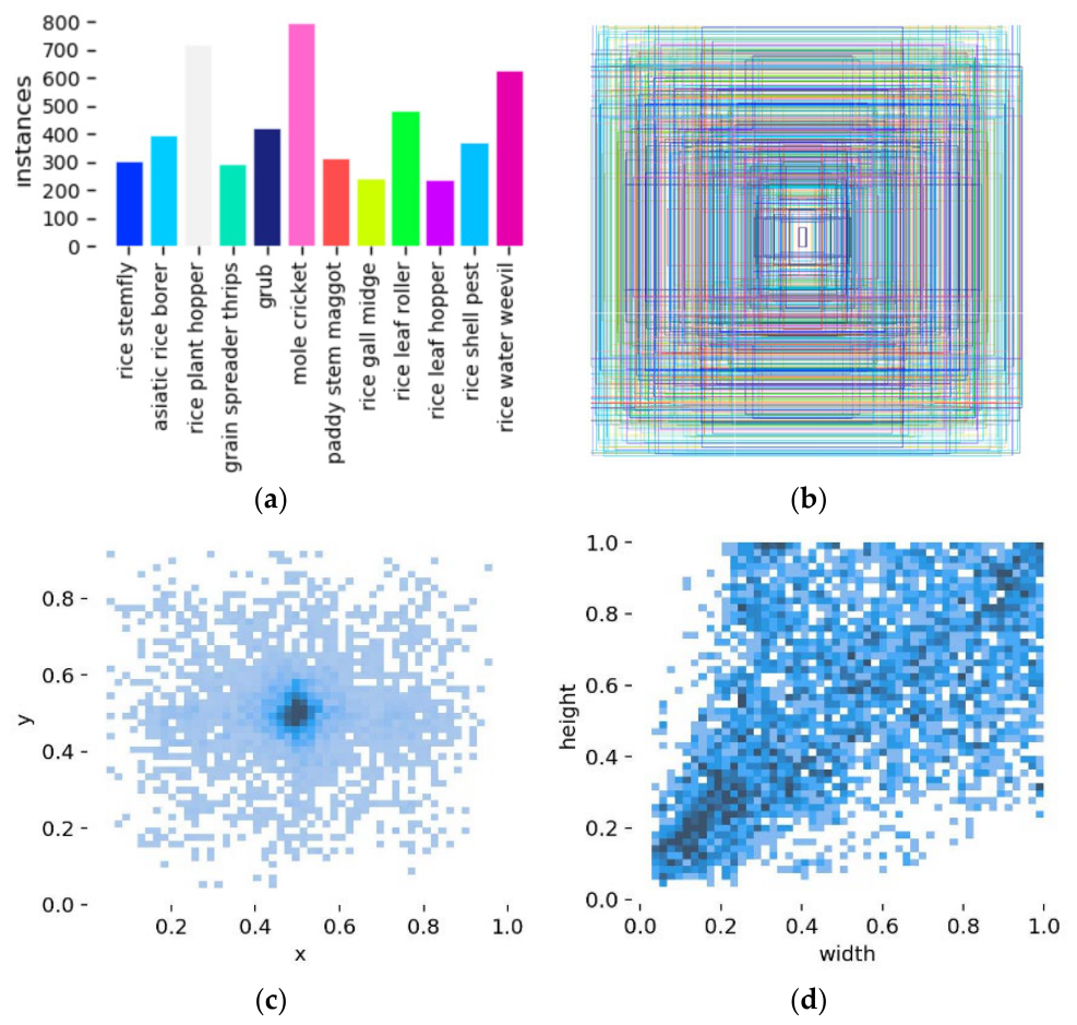
Figure 1 visualizes the structural distribution of the compiled dataset. Specifically, Figure 1a,b detail the per-category instance counts and bounding box dimensions, exposing a severe class imbalance alongside a heavy concentration of small-to-medium targets. Furthermore, the spatial and dimensional analyses in Figure 1c,d reveal that these targets heavily cluster near the image center, maintaining width-to-height ratios predominantly between 0 and 0.4.

2.2. Image Preprocessing

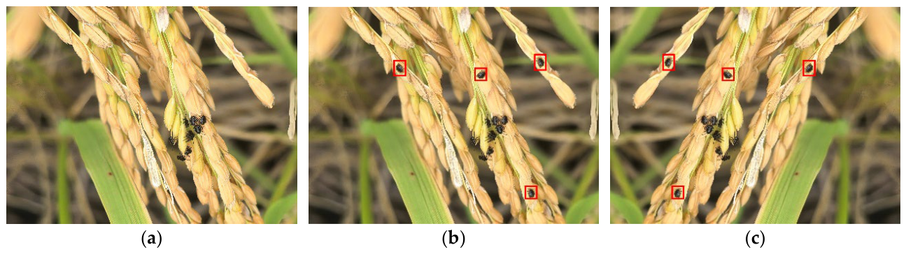
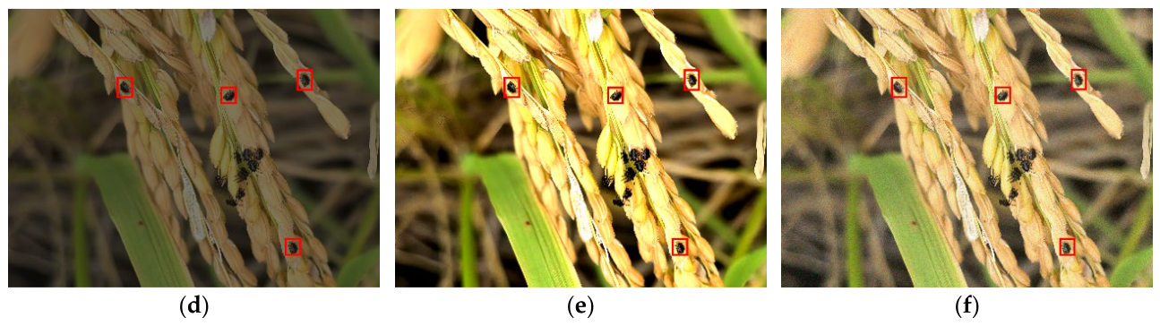
As detailed in Table 2, offline targeted augmentation was applied only to minority-class samples in the training set. Object cropping was centered on annotated pest boxes, with crop dimensions randomly sampled from 1.0 to 1.2 times the bounding-box size; box coordinates were then recalculated in the cropped image. Scene re-embedding was applied with a probability of 0.25 by pasting cropped pest instances at random positions on alternative paddy-field backgrounds, with a scale factor of 0.8–1.0; bounding boxes were updated according to the new scale and position. Additional augmentations included horizontal flipping (p = 0.5), brightness adjustment (−0.2 to +0.2), contrast adjustment (0.75–1.25), and zero-mean Gaussian noise (σ = 0.05, p = 0.3). Geometric transformations updated bounding-box coordinates accordingly, whereas photometric transformations left them unchanged. Figure 2 shows representative examples of these operations.

Figure 2 illustrates representative sample images following the data augmentation process. Before data augmentation, the 4470 original images were partitioned into training, validation, and test sets at a ratio of 7:2:1. The partitioning was performed at the original-image level, and all images derived from the same original sample were retained within the same subset. For the self-collected images, which were all acquired from the same paddy-field site in Jiangshan City, samples from the same acquisition date and capture session were grouped and assigned to the same subset. For images obtained from the IP102 and PaddlePaddle AI Studio datasets, where detailed acquisition information was not consistently available, the original dataset source and image identity were retained during partitioning.

After dataset partitioning, augmentation was applied exclusively to the training set. The implemented augmentation operations for minority classes enriched the diversity of the training data and increased the representation of underrepresented pest categories, while the validation and test sets consisted solely of unmodified original images. The instance counts before and after augmentation are summarized in

Table 3. Comparison of the Z-RP12 dataset before and after data augmentation.

ID	Pest Species	Before Augmentation		After Augmentation
		Images	Instances	Images	Instances
0	Rice stem fly	93	93	213	305
1	Asiatic rice borer	384	397	384	397
2	Rice plant hopper	705	720	705	720
3	Grain spreader thrips	295	295	295	295
4	Grub	414	421	414	421
5	Mole cricket	798	798	798	798
6	Paddy stem maggot	96	96	287	314
7	Rice gall midge	231	241	231	241
8	Rice leaf roller	472	482	472	482
9	Rice leaf hopper	235	235	235	235
10	Rice shell pest	124	124	343	372
11	Rice water weevil	623	627	623	627
Total		4470	4529	5000	5207

, which details the numerical changes across the 12 rice pest categories. Following training-set augmentation, the total number of images increased to 5000, with 5207 pest instances. The resulting dataset is designated as Z-RP12.

In addition, a separate set of field images acquired using a DJI Osmo Pocket 3 (DJI Technology Co., Ltd., Shenzhen, China) was reserved exclusively for independent evaluation. These images were not included in Z-RP12 and were not used during model training, validation, hyperparameter optimization, or checkpoint selection.

2.3. Proposed Framework PEFF-Net

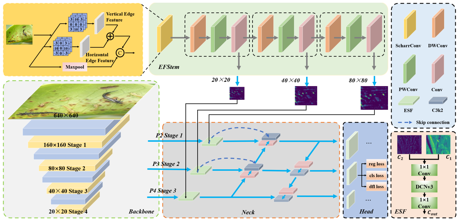
While the YOLO series is a standard paradigm for agricultural object detection, selecting an appropriate baseline requires empirical evaluation. Following a preliminary benchmark of mainstream YOLO architectures, YOLO11n demonstrated the most effective balance of mAP, FLOPs, and parameter efficiency on our dataset. Recent YOLO11n-based rice-pest detectors have already demonstrated the effectiveness of task-oriented scale reconstruction and lightweight feature refinement, including YOLO-RP and GAFNet. Accordingly, PEFF-Net is designed around a different feature-processing objective: explicit construction of shallow structural edge representations, semantic alignment of these representations with deeper backbone features, and lightweight cross-layer aggregation for small-target prediction. As detailed in Figure 3, EFStem and ESF jointly upgrade the backbone to establish the edge-to-semantic feature pathway, while LCFO refines the prediction hierarchy to reduce structural redundancy and coordinate multi-scale information flow for edge deployment.

2.3.1. Edge Feature Extraction Stem (EFStem)

In the context of rice pest detection, repeated downsampling in conventional convolutional networks can progressively weaken fine-grained structural information, thereby affecting the localization of small targets. To preserve and propagate these structural cues across different feature scales, the proposed EFStem explicitly extracts edge information from high-resolution shallow representations and progressively constructs multi-scale edge features. Through successive depthwise and pointwise convolution operations, EFStem generates edge representations at spatial resolutions of 80 × 80, 40 × 40, and 20 × 20, which are aligned with the corresponding hierarchical backbone features for subsequent edge-semantic fusion.

As illustrated in Figure 3, EFStem starts from the high-resolution shallow representation X, which is first fed into the ScharrConv component to extract explicit structural information. ScharrConv adopts a dual-branch parallel architecture. Specifically, one branch extracts horizontal and vertical edge responses using predefined Scharr operators, while the complementary branch preserves salient spatial information through max-pooling operations. The Scharr operator is a classical edge detection mechanism, wherein the horizontal convolution kernel $G_x$ and the vertical convolution kernel $G_y$ are defined as follows:

$$S_x=\left[\begin{array}{ccc}-3& 0& 3\\ -10& 0& 10\\ -3& 0& 3\end{array}\right],S_y=\left[\begin{array}{ccc}-3& -10& -3\\ 0& 0& 0\\ 3& 10& 3\end{array}\right]$$

(1)

Following the dual-branch processing, the extracted edge features and the spatially enriched features are concatenated along the channel dimension, yielding a unified feature map $X_e$ that integrates both edge and spatial information:

$$X_e=\mathrm{C}\mathrm{o}\mathrm{n}\mathrm{c}\mathrm{a}\mathrm{t}(\left({\mathrm{S}\mathrm{c}\mathrm{h}\mathrm{a}\mathrm{r}\mathrm{r}}_x\left({\mathrm{C}\mathrm{o}\mathrm{n}\mathrm{v}}_{3\times 3}\left(X\right)\right)\right)⨁{(\mathrm{S}\mathrm{c}\mathrm{h}\mathrm{a}\mathrm{r}\mathrm{r}}_y({\mathrm{C}\mathrm{o}\mathrm{n}\mathrm{v}}_{3\times 3}\left(X\right)\left)\right),\mathrm{M}\mathrm{a}\mathrm{x}\mathrm{p}\mathrm{o}\mathrm{o}\mathrm{l}\left({\mathrm{C}\mathrm{o}\mathrm{n}\mathrm{v}}_{3\times 3}\right(X\left)\right))$$

(2)

Among them, ${\mathrm{C}\mathrm{o}\mathrm{n}\mathrm{v}}_{3\times 3}$ denotes the 3 × 3 convolutional layer, ${\mathrm{S}\mathrm{c}\mathrm{h}\mathrm{a}\mathrm{r}\mathrm{r}}_x$ and ${\mathrm{S}\mathrm{c}\mathrm{h}\mathrm{a}\mathrm{r}\mathrm{r}}_y$ represent the features extracted by the Scharr operators in the horizontal and vertical directions, respectively, and $⨁$ denotes element-wise addition.

Assuming the feature map obtained after the ScharrConv operation is denoted as $X_e$, the EFStem module utilizes it as the foundational input for the subsequent generation of multi-scale edge features. To obtain multi-scale edge representations that are spatially aligned with the deeper feature maps, this architecture sequentially stacks depthwise separable convolutions and pointwise convolutions. While progressively reducing the spatial resolution of the feature maps, this design concurrently reinforces the contextual information and the fine-grained detail representation of small pest targets:

$${X_e}^{\prime }=P\left(T_k\right(X_e\left)\right)$$

(3)

$${X_e}^{″}=P\left(T_k\right({X_e}^{\prime }\left)\right)$$

(4)

$${X_e}^{‴}=P\left(T_k\right({X_e}^{″}\left)\right)$$

(5)

Among them, $T_k$ denotes a Depthwise Convolution (DWConv) with a kernel size of $k$, and $P$ represents a Pointwise Convolution (PWConv). In this paper, $k$ = 3. The outputs ${X_e}^{\prime }$, ${X_e}^{″}$, and ${X_e}^{‴}$ correspond to the 80 × 80, 40 × 40, and 20 × 20 edge representations, respectively.

The EFStem module progressively generates three scale-specific edge representations through a cascaded sequence of DWConv and PWConv operations. Specifically, ${X_e}^{\prime }$, ${X_e}^{″}$, and ${X_e}^{‴}$ correspond to edge feature maps with spatial resolutions of 80 × 80, 40 × 40, and 20 × 20, respectively. These multi-scale edge representations are subsequently aligned with the corresponding hierarchical backbone features for edge-semantic fusion.

2.3.2. Edge Semantic Fusion Module (ESF)

Although EFStem explicitly captures structural boundary information, these shallow geometric edge features are intrinsically heterogeneous at the semantic level relative to the deeper contextual features generated by the backbone network. Direct concatenation or linear fusion can therefore introduce feature conflict and disrupt the original semantic flow. To address this representation mismatch, we propose the Edge Semantic Fusion (ESF) module, which performs channel-level interaction and adaptive spatial modeling to align shallow structural boundaries with deep contextual semantics. The architecture of ESF is illustrated in Figure 3.

Architecturally, the ESF adopts an improved “dimension reduction-expansion” paradigm while simultaneously incorporating deformable convolutions. This design not only efficiently merges heterogeneous features but also adaptively adjusts the receptive field, thereby preserving the morphological flexibility required for detecting irregularly shaped pests. Given the feature map from the backbone network, denoted as $X_1$, and the edge features, denoted as $X_2$, the unit first aggregates them along the channel axis:

$$X_{cat}=\mathrm{C}\mathrm{o}\mathrm{n}\mathrm{c}\mathrm{a}\mathrm{t}(X_1,X_2)$$

(6)

Subsequently, the aggregated feature map undergoes a three-stage cascaded transformation to achieve deep integration:

$$X_{out}={\mathrm{C}\mathrm{o}\mathrm{n}\mathrm{v}}_{1\times 1}\left(\mathrm{D}\mathrm{C}\mathrm{N}\mathrm{v}3\right({\mathrm{C}\mathrm{o}\mathrm{n}\mathrm{v}}_{1\times 1}\left(X_{cat}\right)\left)\right)$$

(7)

In Equation (7), the input channels are initially halved via a 1 × 1 convolutional layer, which substantially mitigates the parameter volume and computational load for subsequent modules, thereby bolstering overall computational efficiency. Following this, traditional static convolutions are eschewed in the feature extraction phase in favor of Deformable Convolution version 3 (DCNv3) [19]. By dynamically modulating spatial sampling locations, DCNv3 can meticulously distort its receptive field to conform closely to the asymmetric and intricate morphological boundaries of agricultural pests. Simultaneously, it effectively evades the linear high-frequency noise interference commonly induced by rice leaf veins. The terminal ${\mathrm{C}\mathrm{o}\mathrm{n}\mathrm{v}}_{1\times 1}$ is then tasked with remapping the channel count to restore the original feature dimensionality. Overall, this hourglass architecture, coupled with deformable operations, is designed to reduce computational overhead while retaining morphology-aware feature representation.

2.3.3. Lightweight Cross-Layer Feature Fusion Output Module (LCFO)

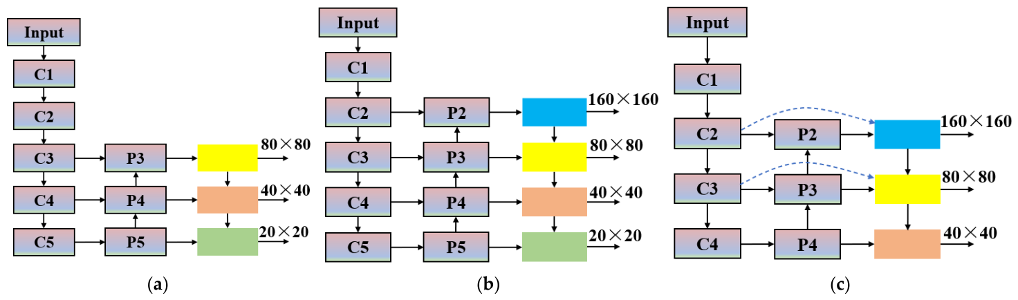
Although EFStem and ESF enhance fine-grained edge-to-semantic representations, the default multi-scale prediction hierarchy of YOLO11n is not fully aligned with the target-scale distribution of Z-RP12, which is dominated by small and medium-sized pests. As illustrated in Figure 4a, the original YOLO11n predicts from P3, P4, and P5 feature maps with spatial resolutions of 80 × 80, 40 × 40, and 20 × 20, respectively. The low-resolution P5 branch provides a large receptive field but retains limited spatial detail for small targets, whereas shallower high-resolution features preserve richer localization information.

To better match this scale distribution, a high-resolution 160 × 160 P2 prediction branch is first introduced to enhance the representation of fine-grained spatial information, forming the YOLO11n-P2 structure shown in Figure 4b. Building on this configuration, the proposed Lightweight Cross-layer Feature Fusion Output (LCFO) module removes the low-resolution P5 prediction branch and retains the P2, P3, and P4 prediction hierarchy, as illustrated in Figure 4c. Cross-layer connections are further introduced to aggregate shallow spatial details with deeper semantic representations. Through this design, LCFO enhances cross-scale information interaction while reducing redundant deep-scale computation, providing a compact feature-fusion and prediction structure for small-pest detection.

2.4. Design of the Rice Pest Detection System

2.4.1. Edge Device Parameters

In this study, the model was deployed on a Jetson Orin Nano Super 8 GB edge device, which is based on the NVIDIA Ampere GPU architecture. The detailed hardware performance parameters are summarized in

Table 4. Technical Specifications of NVIDIA Jetson Orin Nano Super 8 GB.

Parameters	Configuration
AI Performance	67 TOPS
GPU	NVIDIA Ampere architecture with 1024 CUDA cores and 32 tensor cores
CPU	6-core Arm® Cortex®-A78AE v8.2 64-bit CPU 1.5 MB L2 + 4 MB L3
Memory	8 GB 128-bit LPDDR5, 102 GB/s
Power	7 W–25 W

.

As shown in Table 4, the device delivers a peak INT8 AI computing performance of 67 TOPS, a memory bandwidth of 102 GB/s, and multi-channel high-definition video-decoding capabilities, providing sufficient computational resources for the deployment experiments in this study. Its configurable power range spans from 7 W to 25 W, supporting operation under varying computational workloads and making it suitable for the edge-deployment scenarios evaluated in this work. The Linux runtime environment configuration for the NVIDIA Jetson Orin Nano Super 8 GB is detailed in

Table 5. Configuration of Linux Operating Environment.

Configuration	Version
Operating System	Ubuntu 22.04 LTS
Jetpack SDK	6.2
CUDA Toolkit	12.6
cuDNN	9.3.0
TensorRT	10.3.0

.

2.4.2. TensorRT Implementation of the DCNv3 Operator

The ESF employs DCNv3 to adaptively aggregate edge-aware features at dynamically sampled locations. However, DCNv3 is not directly represented as a native operator in the TensorRT deployment pipeline used in this study, which requires additional handling during model conversion. To address this, we adopted an operator decomposition strategy during ONNX export. Specifically, the DCNv3 module is decomposed into standard operators supported by TensorRT: the offset prediction branch is implemented as a 1 × 1 convolution, the sampling and interpolation operations are mapped to the GridSample operator, and the weighted feature aggregation is realized via element-wise multiplication followed by standard convolution. This decomposition enables the model to be converted to a TensorRT engine without introducing a custom TensorRT plugin, while preserving the functional behavior of the DCNv3-based feature-processing pathway.

2.4.3. Development of the Rice Pest Detection System

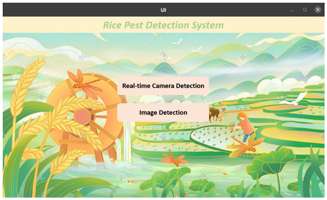
To bridge the gap between algorithmic design and practical application, we engineered a custom rice pest detection system utilizing the PyQt5 framework. As illustrated in Figure 5, the graphical user interface supports both real-time camera streams and static image analysis. Furthermore, this lightweight software architecture ensures seamless deployment across standard desktop environments and resource-constrained edge devices.

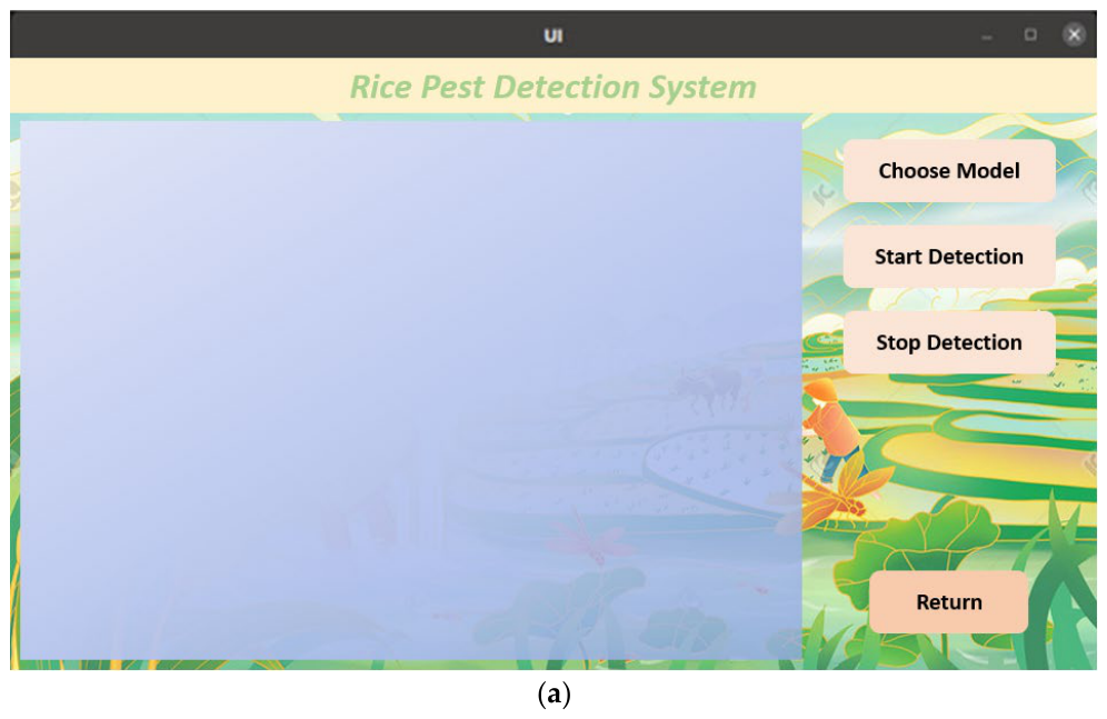
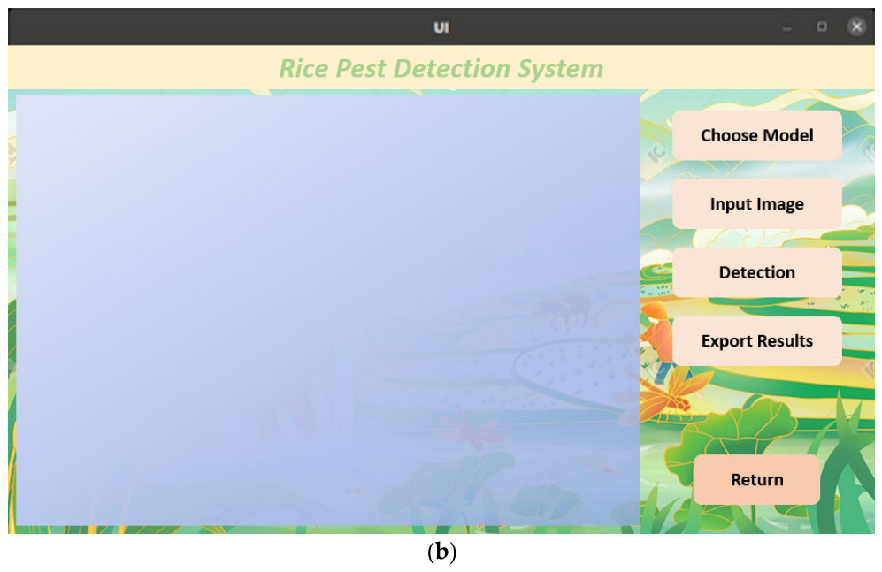
The main interface offers a straightforward navigation hub, allowing users to transition seamlessly between real-time camera monitoring and static image analysis. As detailed in Figure 6a, the real-time detection mode partitions the workspace into a left-hand visualization panel for live video streams and a right-hand control module. This command section enables users to dynamically select detection models, toggle the inference pipeline, and return to the primary menu. Maintaining architectural symmetry, the single-image detection interface presented in Figure 6b employs an identical dual-panel layout. Instead of a continuous video feed, this mode integrates specialized functions for loading local image files, executing static inference, and exporting the resulting diagnostic data for downstream analysis.

3. Experiment and Analysis

3.1. Experimental Environment Configuration and Deployment Platform

The experiments in this study were conducted on the Windows 10 system, with the following hardware configurations: CPU as i5-14600KF@3.50 GHz, RAM as 32 G, GPU as NVIDIA GeForce RTX4070 Ti SUPER, and VRAM as 16 G. The programming platform was Pycharm 2024.3.1, with development carried out using Python 3.12.9, and the CUDA version was 12.6. The model was trained based on the deep learning framework PyTorch 2.6.0. The experimental parameter configurations are shown in

Table 6. Configuration of the experimental hyperparameters.

Hyperparameter	Configuration
Model Type	YOLO11n (baseline)
Training epochs	300
Batch size	16
Image size	640 × 640
Optimizer	SGD
Initial learning rate	0.01
Final learning rate	0.0001
Momentum	0.937
Weight decay	0.0005
Workers	4

.

During model training, the default Ultralytics YOLO11 online augmentation configuration was retained: hsv_h = 0.015, hsv_s = 0.7, hsv_v = 0.4, translate = 0.1, scale = 0.5, fliplr = 0.5, and mosaic = 1.0. Rotation (degrees = 0.0), vertical flipping (flipud = 0.0), shear (shear = 0.0), perspective transformation (perspective = 0.0), MixUp (mixup = 0.0), and BGR channel swapping (bgr = 0.0) were disabled. Mosaic augmentation was disabled during the final 10 training epochs (close_mosaic = 10).

For reproducibility, the remaining training and inference settings followed the Ultralytics YOLO11 defaults unless otherwise specified in Table 6. Pretrained initialization was enabled using the official COCO-pretrained YOLO11n checkpoint (yolo11n.pt; pretrained = True); newly introduced PEFF-Net layers without corresponding pretrained parameters used the framework default initialization. During validation, the confidence threshold was 0.001. For prediction and field deployment, the confidence threshold was 0.25. Non-Maximum Suppression (NMS) used an IoU threshold of 0.70, a maximum of 300 detections per image (max_det = 300), and class-aware suppression (agnostic_nms = False). For each independent training run, the Ultralytics best.pt checkpoint corresponding to the highest validation mAP@0.5:0.95 was retained for final test evaluation; neither the Z-RP12 test set nor the independent field test set was used for checkpoint selection or hyperparameter optimization. The same validation and post-processing settings were applied to all compared models.

3.2. Evaluation Metrics

This study uses precision, recall, ${\mathrm{m}\mathrm{A}\mathrm{P}}_{0.5}$, and ${\mathrm{m}\mathrm{A}\mathrm{P}}_{0.5:0.95}$ to evaluate the accuracy of the model in rice pest detection, with the calculation methods detailed in Formulas (8)–(11). Secondly, to comprehensively evaluate the performance of the model, this study also introduces the following evaluation indicators: parameters, FLOPs, model size, and Frames Per Second (FPS), which further reflect the model’s performance in terms of computational efficiency and resource consumption.

$$\mathrm{R}\mathrm{e}\mathrm{c}\mathrm{a}\mathrm{l}\mathrm{l}={\displaystyle \frac{\mathrm{T}\mathrm{P}}{\mathrm{T}\mathrm{P}+\mathrm{F}\mathrm{N}}}$$

(8)

$$\mathrm{P}\mathrm{r}\mathrm{e}\mathrm{c}\mathrm{i}\mathrm{s}\mathrm{i}\mathrm{o}\mathrm{n}={\displaystyle \frac{\mathrm{T}\mathrm{P}}{\mathrm{T}\mathrm{P}+\mathrm{F}\mathrm{P}}}$$

(9)

$$\mathrm{A}\mathrm{P}={\int }_0^{1}P\left(R\right)dR$$

(10)

$$\mathrm{m}\mathrm{A}\mathrm{P}={\displaystyle \frac{1}{C}}{\displaystyle \sum _{i=1}^C}\mathrm{A}{\mathrm{P}}_i$$

(11)

Among them, TP represents the correctly predicted true positives, FP represents the false positives that are incorrectly predicted as positives, and FN represents the false negatives that are incorrectly predicted as negatives. C denotes the number of categories. ${\mathrm{m}\mathrm{A}\mathrm{P}}_{0.5}$ represents the average precision at an IoU threshold of 0.5, which is used to evaluate the overall detection accuracy. ${\mathrm{m}\mathrm{A}\mathrm{P}}_{0.5:0.95}$ denotes the average precision over the IoU threshold range from 0.5 to 0.95, imposing stricter requirements on target localization.

To further analyze detection performance across different target scales, pest instances were divided into small, medium, and large objects according to their bounding-box areas. Because the images were obtained from multiple sources with different native resolutions, all bounding boxes were mapped to the 640 × 640 evaluation input space before scale assignment. Using COCO-style area thresholds, objects with bounding-box area A < 32² were categorized as small, those with 32² ≤ A < 96² as medium, and those with A ≥ 96² as large, where A = w × h is measured in pixels. Scale-specific AP was subsequently calculated over IoU thresholds from 0.50 to 0.95 for the small, medium, and large object groups, denoted as ${\mathrm{A}\mathrm{P}}_{\mathrm{s}}$, ${\mathrm{A}\mathrm{P}}_{\mathrm{m}}$, and ${\mathrm{A}\mathrm{P}}_l$, respectively.

3.3. Experimental Results

To rigorously validate the proposed architectural enhancements, we conducted comprehensive comparative evaluations under strictly controlled protocols. To guarantee empirical reliability and reproducibility, all procedures adhered to the following standards:

• The statistical results were calculated directly from the unrounded run-level outputs of the three independent experiments. The same random seed assignments (Seed 0, Seed 4, and Seed 6) were consistently maintained across all comparison and ablation experiments. The mean and sample standard deviation were calculated as:

  $$\overline{x}={\displaystyle \frac{1}{n}}{\displaystyle \sum _{i=1}^n}{x}_i$$

  (12)

  $$SD=\sqrt{{\displaystyle \frac{{\sum }_{i=1}^n{(x_i-\overline{x})}^2}{n-1}}}$$

  (13)

  where n = 3 represents the number of independent runs. The 95% confidence intervals (CIs) were calculated using the student’s t distribution:

  $${CI}_{95\%}=\overline{x}\pm t_{0.975,n-1{\displaystyle \frac{SD}{\sqrt{n}}}}$$

  (14)

  where $t_{0.975,2}$ = 4.303 is the critical value of the student’s t distribution. Due to space limitations, the detailed seed-level results and corresponding confidence intervals are provided in the Supplementary Material.
• Standardized Edge Benchmarking: Edge-device performance was measured under a consistent runtime configuration using the same benchmarking procedure for all evaluated models.
• FPS Reporting Scope: The FPS metrics documented in this section reflect desktop GPU performance to establish a relative computational baseline. They do not represent the final operational throughput on the Jetson Orin Nano Super 8 GB edge device.

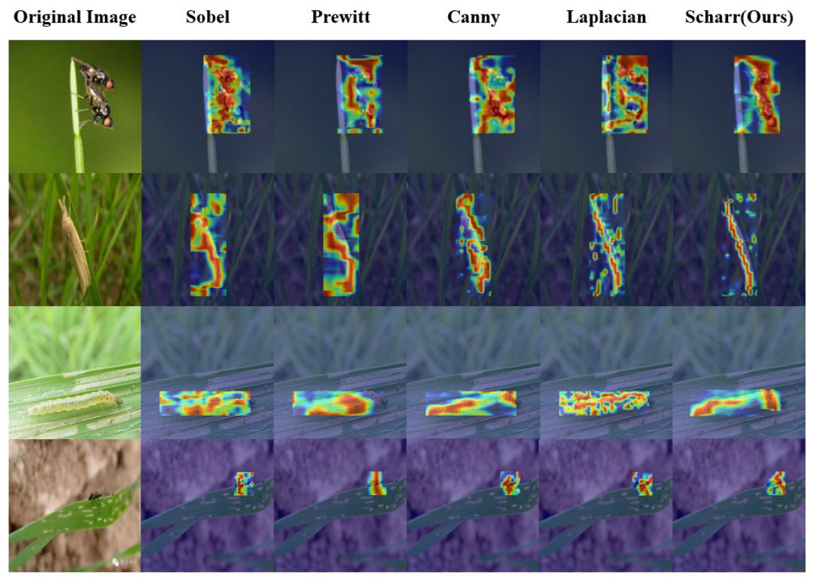
Additionally, Grad-CAM [20] was utilized to visualize the spatial attention of the network. The resulting heatmaps employ a spectral gradient where red zones correspond to high-response focal regions critical for target localization, and blue indicates areas of negligible feature activation.

3.3.1. Comparative Experiments of Different Edge Detection Operators

Table 7. Comparison Results of Different Edge Detection Operators On the Z-RP12 dataset.

Edge Kernel	P (%)	R (%)	${\mathbf{m}\mathbf{A}\mathbf{P}}_{0.5}$ (%)	${\mathbf{m}\mathbf{A}\mathbf{P}}_{0.5:0.95}$ (%)	Param (M)	FLOPs (G)
Sobel	88.1 ± 0.25	79.6 ± 0.28	87.8 ± 0.24	68.1 ± 0.32	2.84	7.2
Prewitt	88.5 ± 0.24	80.0 ± 0.27	88.1 ± 0.23	68.4 ± 0.31	2.84	7.2
Canny	88.3 ± 0.26	79.8 ± 0.29	88.0 ± 0.25	68.4 ± 0.30	2.84	7.2
Laplacian	88.2 ± 0.20	79.9 ± 0.30	87.9 ± 0.27	68.3 ± 0.35	2.84	7.2
Scharr	89.4 ± 0.17	80.5 ± 0.23	88.4 ± 0.18	68.8 ± 0.24	2.84	7.2

compares different edge detection operators integrated into the EFStem module to evaluate the selection of the Scharr operator. The Sobel, Prewitt, Canny, Laplacian, and Scharr edge maps were generated using OpenCV under the same preprocessing protocol. The Canny operator was implemented as a fixed image-processing operation with lower and upper hysteresis thresholds of 50 and 150, respectively. Since these edge operators only replace the edge extraction operation and do not modify the learnable network architecture, the reported parameters and FLOPs remain identical across variants. The computational cost of these fixed image-processing operations was excluded from the network-level FLOPs calculation.

As detailed in Table 7, changing the edge detection operator results in relatively small performance variations without altering the parameter count or FLOPs. Among the evaluated operators, the Scharr variant achieves the highest Precision, Recall, ${\mathrm{m}\mathrm{A}\mathrm{P}}_{0.5}$, and ${\mathrm{m}\mathrm{A}\mathrm{P}}_{0.5:0.95}$, reaching 89.4%, 80.5%, 88.4%, and 68.8%, respectively.

These results suggest that the Scharr operator is more effective for the edge-feature extraction setting evaluated in this study. Its sensitivity to weak edges and fine textures may contribute to the preservation of structural information such as leaf boundaries and pest contours during subsequent feature fusion.

Figure 7 further presents Grad-CAM visualizations for the different edge operators. In the illustrated examples, the Scharr-integrated model exhibits relatively concentrated responses around pest regions and their contours compared with the other evaluated variants, providing qualitative support for the quantitative results in Table 7.

3.3.2. Performance Comparison of Different Backbone Networks

Table 8. Performance comparison of different backbone configurations within the YOLO11n framework on the Z-RP12 dataset.

Backbone	P (%)	R (%)	${\mathbf{m}\mathbf{A}\mathbf{P}}_{0.5}$ (%)	${\mathbf{m}\mathbf{A}\mathbf{P}}_{0.5:0.95}$ (%)	Param (M)	FLOPs (G)	FPS
YOLO11n	86.2 ± 0.21	77.9 ± 0.26	86.1 ± 0.19	65.7 ± 0.28	2.58	6.3	101
StarNet [21]	84.1 ± 0.23	75.7 ± 0.30	82.8 ± 0.24	63.1 ± 0.32	1.94	5.0	121
EfficientViT [22]	89.9 ± 0.25	76.1 ± 0.32	85.2 ± 0.26	65.4 ± 0.35	3.74	7.9	103
FasterNet [23]	87.2 ± 0.22	78.5 ± 0.27	85.9 ± 0.20	66.3 ± 0.26	3.91	9.2	105
MobileNet-V4 [24]	84.6 ± 0.24	75.2 ± 0.31	82.3 ± 0.23	63.0 ± 0.30	5.43	21.0	84
ResNet-18 [25]	90.1 ± 0.30	78.6 ± 0.35	85.7 ± 0.28	65.8 ± 0.37	13.06	33.6	55
Vision Mamba [26]	90.7 ± 0.28	79.4 ± 0.32	86.5 ± 0.31	66.2 ± 0.35	18.21	48.1	50
Ours (EFStem + ESF)	90.3 ± 0.20	81.2 ± 0.21	89.6 ± 0.23	69.5 ± 0.26	2.91	7.8	78

compares different backbone configurations within the YOLO11n framework, while retaining the original YOLO11n neck and detection head, to isolate and evaluate the effect of backbone design.

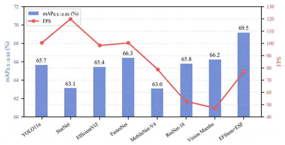
Table 8 demonstrates that directly replacing the YOLO11n backbone with mainstream lightweight networks fails to effectively balance detection accuracy and model complexity. For instance, Vision Mamba achieves an ${\mathrm{m}\mathrm{A}\mathrm{P}}_{0.5}$ of 86.5% but yields a larger parameter count of 18.21 M and a lower inference speed of 50 FPS. In contrast, FasterNet delivers a higher inference speed of 105 FPS, while its ${\mathrm{m}\mathrm{A}\mathrm{P}}_{0.5}$ of 85.9% is slightly lower than the 86.1% baseline. Among all compared backbone schemes, the proposed EFStem–ESF backbone achieves superior comprehensive detection performance, with a Precision of 90.3%, Recall of 81.2%, ${\mathrm{m}\mathrm{A}\mathrm{P}}_{0.5}$ of 89.6%, and ${\mathrm{m}\mathrm{A}\mathrm{P}}_{0.5:0.95}$ of 69.5%. Compared with the original YOLO11n backbone, it improves ${\mathrm{m}\mathrm{A}\mathrm{P}}_{0.5}$ and ${\mathrm{m}\mathrm{A}\mathrm{P}}_{0.5:0.95}$ by 3.5 and 3.8 percentage points, respectively, while retaining a feasible inference speed of 78 FPS. These results verify that the designed EFStem–ESF backbone enhances feature representation capability and improves detection accuracy across the evaluated metrics, leading to a favourable accuracy-performance trade-off for pest detection tasks.

To visually illustrate this performance-efficiency trade-off, Figure 8 presents a dual-axis chart plotting detection accuracy against inference speed using data from Table 8. The visualization shows that the proposed EFStem–ESF backbone yields considerably higher detection accuracy than alternative backbone configurations, while maintaining acceptable real-time inference throughput.

3.3.3. Validation Experiment of the Effectiveness of LCFO

To evaluate the effectiveness of the LCFO, comparative experiments were conducted using YOLO11n, YOLO11n-P2, YOLO-LCFO without cross-layer connections, and the complete YOLO-LCFO. The results are presented in

Table 9. Performance Comparison of Different Neck Networks On the Z-RP12 dataset.

Head	P (%)	R (%)	${\mathbf{m}\mathbf{A}\mathbf{P}}_{0.5}$ (%)	${\mathbf{m}\mathbf{A}\mathbf{P}}_{0.5:0.95}$ (%)	Param (M)	FLOPs (G)	FPS
YOLO11n	86.2 ± 0.21	77.9 ± 0.26	86.1 ± 0.19	65.7 ± 0.28	2.58	6.3	101
YOLO11n-P2	86.9 ± 0.23	79.4 ± 0.27	87.6 ± 0.21	67.5 ± 0.30	2.68	9.4	92
YOLO-LCFO (without cross-layer connections)	86.5 ± 0.14	79.1 ± 0.16	87.2 ± 0.18	67.1 ± 0.21	1.83	5.6	110
YOLO-LCFO	87.1 ± 0.17	79.6 ± 0.15	87.7 ± 0.16	67.9 ± 0.18	1.95	5.9	106

.

Compared with the YOLO11n baseline, YOLO-LCFO improves Precision from 86.2% to 87.1%, Recall from 77.9% to 79.6%, ${\mathrm{m}\mathrm{A}\mathrm{P}}_{0.5}$ from 86.1% to 87.7%, and ${\mathrm{m}\mathrm{A}\mathrm{P}}_{0.5:0.95}$ from 65.7% to 67.9%. Meanwhile, the parameter counts decreases from 2.58 M to 1.95 M and the FLOPs decrease from 6.3 G to 5.9 G, while the inference speed increases from 101 FPS to 106 FPS. These results indicate that the modified prediction hierarchy improves small-target detection performance while maintaining a compact computational structure.

Compared with YOLO11n-P2, YOLO-LCFO achieves slightly higher Precision, Recall, ${\mathrm{m}\mathrm{A}\mathrm{P}}_{0.5}$, and ${\mathrm{m}\mathrm{A}\mathrm{P}}_{0.5:0.95}$, while reducing the parameter count from 2.68 M to 1.95 M and the FLOPs from 9.4 G to 5.9 G. The inference speed also increases from 92 FPS to 106 FPS. This suggests that removing the low-resolution P5 prediction branch helps offset part of the computational overhead introduced by the P2 branch while maintaining the high-resolution prediction capability required for small pest targets.

The effect of cross-layer connections can be further observed by comparing YOLO-LCFO with the variant without cross-layer connections. Introducing cross-layer fusion increases the parameter count from 1.83 M to 1.95 M and the FLOPs from 5.6 G to 5.9 G, while improving Precision by 0.6 percentage points, Recall by 0.5 percentage points, ${\mathrm{m}\mathrm{A}\mathrm{P}}_{0.5}$ by 0.5 percentage points, and ${\mathrm{m}\mathrm{A}\mathrm{P}}_{0.5:0.95}$ by 0.8 percentage points. These results show that the cross-layer connections contribute additional detection gains by strengthening the interaction between shallow spatial information and deeper semantic features, with a relatively small increase in model complexity.

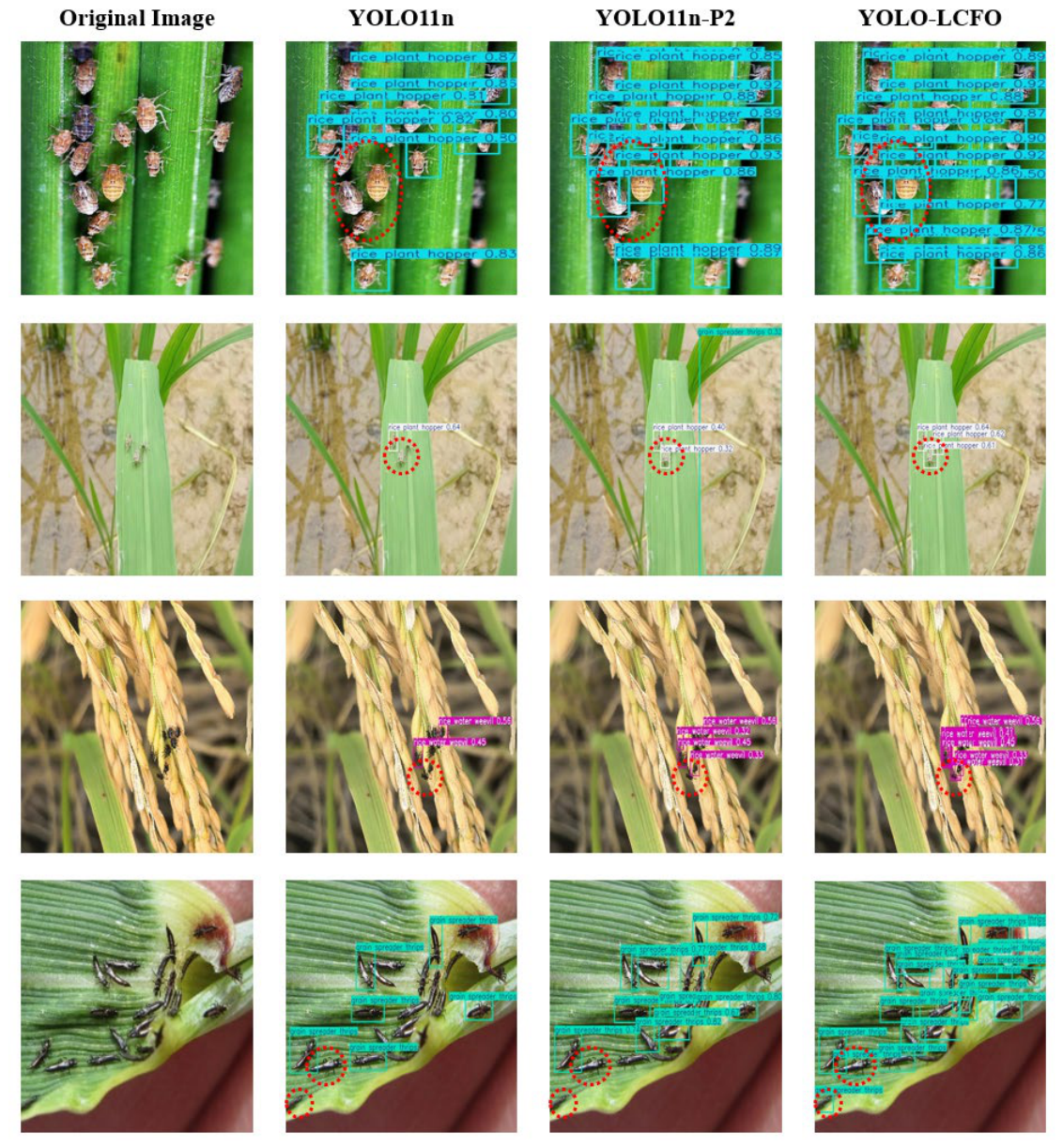
Figure 9 further illustrates representative detection results for the different prediction structures. Compared with YOLO11n, the YOLO11n-P2 variant reduces some missed detections of small targets, while the complete YOLO-LCFO provides improved localization and confidence in the illustrated examples. Together with the quantitative results in Table 9, these observations support the effectiveness of the proposed cross-layer feature fusion strategy for small rice pest detection.

3.3.4. Ablation Experiments

To thoroughly evaluate the contribution of each proposed module to the model’s detection performance, an ablation study was conducted based on the YOLO11n baseline model. In this context, “$ℛ$” indicates the adoption of the respective improvement strategy, whereas “-” denotes its omission. The ablation results of the various modules evaluated on the Z-RP12 dataset are detailed in

Table 10. Ablation Experiments On the Z-RP12 dataset.

EFStem	ESF	LCFO	P (%)	R (%)	${\mathbf{m}\mathbf{A}\mathbf{P}}_{0.5}$ (%)	${\mathbf{m}\mathbf{A}\mathbf{P}}_{0.5:0.95}$ (%)	Param (M)	FLOPs (G)	Size (MB)	FPS
-	-	-	86.2 ± 0.21	77.9 ± 0.26	86.1 ± 0.19	65.7 ± 0.28	2.58	6.3	5.3	101
$ℛ$	-	-	89.4 ± 0.17	80.5 ± 0.23	88.4 ± 0.18	68.8 ± 0.24	2.84	7.2	6.0	89
$ℛ$	$ℛ$	-	90.3 ± 0.20	81.2 ± 0.21	89.6 ± 0.23	69.5 ± 0.26	2.91	7.8	7.1	78
-	-	$ℛ$	87.1 ± 0.17	79.6 ± 0.15	87.7 ± 0.16	67.9 ± 0.18	1.95	5.9	2.6	106
$ℛ$	-	$ℛ$	90.1 ± 0.23	80.8 ± 0.26	89.0 ± 0.27	69.2 ± 0.31	2.04	6.8	3.2	98
$ℛ$	$ℛ$	$ℛ$	91.5 ± 0.15	82.6 ± 0.13	90.6 ± 0.17	70.4 ± 0.10	2.12	7.5	3.6	80

.

Table 10 confirms that each individual architectural modification exerts distinct influences on overall model performance. Integrating EFStem alone boosts Precision, Recall, ${\mathrm{m}\mathrm{A}\mathrm{P}}_{0.5}$, and ${\mathrm{m}\mathrm{A}\mathrm{P}}_{0.5:0.95}$ by 3.2%, 2.6%, 2.3%, and 3.1%, respectively, validating its capacity to extract and reinforce critical edge semantics, despite a slight throughput reduction to 89 FPS. Building upon this, the ESF effectively fuses these shallow edge features into deeper semantic representations, further elevating ${\mathrm{m}\mathrm{A}\mathrm{P}}_{0.5}$ to 89.6% and ${\mathrm{m}\mathrm{A}\mathrm{P}}_{0.5:0.95}$ to 69.5%. Conversely, deploying the LCFO independently optimizes structural efficiency. It yields gains across all accuracy metrics while reducing the parameter footprint by 24.4% and accelerating inference to 106 FPS. When all three modules are combined, the resulting PEFF-Net achieves the best performance among these ablation configurations. Compared with the YOLO11n baseline, it obtains notable improvements: 5.3% in Precision, 4.7% in Recall, 4.5% in ${\mathrm{m}\mathrm{A}\mathrm{P}}_{0.5}$, and 4.7% in ${\mathrm{m}\mathrm{A}\mathrm{P}}_{0.5:0.95}$. Meanwhile, the model size is reduced by 1.7 MB with 0.46 M fewer parameters, maintaining 80 FPS inference speed to meet the requirements of real-time agricultural monitoring.

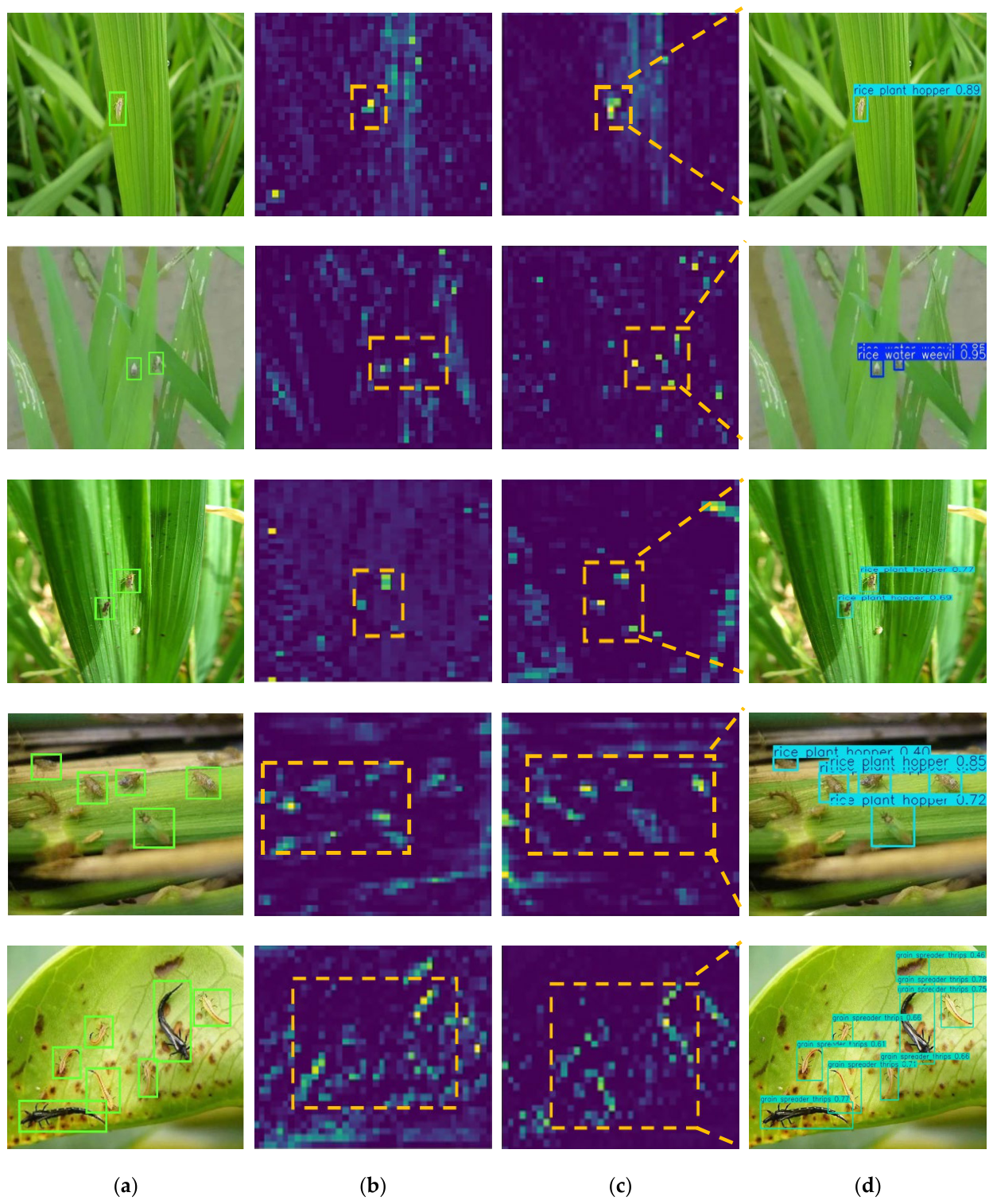
Figure 10 visualizes these comparative detection outcomes against the baseline model. By explicitly propagating spatial fidelity and edge information across the network hierarchy, the PEFF-Net architecture systematically neutralizes the severe background interference that limits standard feature extraction, translating these quantitative gains into highly accurate, localized visual predictions.

3.3.5. Comparison Experiments of Different Object Detection Algorithms

Table 11. Performance Comparison of Different Object Algorithms On the Z-RP12 dataset.

Model	P (%)	R (%)	${\mathbf{m}\mathbf{A}\mathbf{P}}_{0.5}$(%)	${\mathbf{m}\mathbf{A}\mathbf{P}}_{0.5:0.95}$(%)	Param (M)	FLOPs (G)	Size (MB)	FPS
YOLOv5n	75.1 ± 0.23	73.7 ± 0.30	73.2 ± 0.24	56.3 ± 0.32	2.51	7.1	5.1	110
YOLOv6n [27]	79.2 ± 0.25	73.9 ± 0.28	80.2 ± 0.26	61.1 ± 0.30	4.23	11.8	8.3	95
YOLOv8n	86.4 ± 0.22	76.3 ± 0.27	85.7 ± 0.21	64.5 ± 0.29	3.01	8.2	6.0	90
YOLOv9t [28]	86.3 ± 0.23	75.9 ± 0.29	84.8 ± 0.25	64.8 ± 0.31	1.97	7.6	4.5	105
YOLOv10n [29]	85.7 ± 0.22	77.5 ± 0.26	84.9 ± 0.22	65.3 ± 0.28	2.72	8.2	5.5	98
YOLO11n	86.2 ± 0.21	77.9 ± 0.26	86.1 ± 0.19	65.7 ± 0.28	2.58	6.3	5.3	101
YOLOv12n [30]	84.2 ± 0.24	74.5 ± 0.29	82.0 ± 0.24	62.6 ± 0.32	2.51	5.8	5.2	100
YOLOv13n [31]	85.7 ± 0.25	74.3 ± 0.31	81.8 ± 0.27	63.9 ± 0.34	2.45	6.1	5.2	102
Hyper-YOLO [32]	86.5 ± 0.18	80.3 ± 0.15	86.9 ± 0.19	66.7 ± 0.15	3.62	9.5	7.3	85
RT-DETR-R18 [33]	86.0 ± 0.31	72.6 ± 0.35	76.5 ± 0.28	60.3 ± 0.36	19.88	57.0	77.0	35
Faster R-CNN [34]	72.2 ± 0.32	88.0 ± 0.38	87.6 ± 0.33	62.4 ± 0.43	136.9	401.9	-	-
SSD [35]	89.6 ± 0.28	68.7 ± 0.34	82.0 ± 0.26	58.0 ± 0.35	26.28	62.7	-	-
RetinaNet [36]	81.7 ± 0.30	71.2 ± 0.31	80.6 ± 0.27	51.5 ± 0.34	38.9	170.0	-	-
EfficientDet [37]	85.6 ± 0.16	68.1 ± 0.22	81.4 ± 0.20	53.6 ± 0.23	3.87	5.2	-	-
CenterNet [38]	76.9 ± 0.29	79.3 ± 0.33	73.0 ± 0.28	51.8 ± 0.37	32.66	70.2	-	-
Paddy-YOLO [39]	84.8 ± 0.23	77.0 ± 0.28	84.2 ± 0.26	63.5 ± 0.30	3.3	9.1	-	-
RicePest-DETR [40]	87.2 ± 0.19	78.4 ± 0.25	85.3 ± 0.24	65.1 ± 0.25	19.6	65.5	-	-
YOLO-RP	89.3 ± 0.18	85.1 ± 0.22	89.7 ± 0.17	64.2 ± 0.24	1.01	3.2	3.0	97
GAFNet	89.0 ± 0.20	81.8 ± 0.25	87.8 ± 0.19	66.1 ± 0.26	2.45	5.6	5.1	92
PEFF-Net	91.5 ± 0.15	82.6 ± 0.13	90.6 ± 0.17	70.4 ± 0.10	2.12	7.5	3.6	80

compares the proposed PEFF-Net with mainstream object detection algorithms and two closely related YOLO11n-based rice-pest detectors, YOLO-RP and GAFNet. To ensure a fair comparison, YOLO-RP and GAFNet were reimplemented and evaluated on the Z-RP12 dataset using the same dataset split, training protocol, software environment, and hardware configuration as PEFF-Net. Model complexity and inference speed were also measured using the same profiling procedure. The results therefore provide a controlled comparison of detection accuracy and computational efficiency under identical experimental conditions.

As shown in Table 11, PEFF-Net achieves the highest Precision, ${\mathrm{m}\mathrm{A}\mathrm{P}}_{0.5}$, and ${\mathrm{m}\mathrm{A}\mathrm{P}}_{0.5:0.95}$ among the evaluated models, reaching 91.5%, 90.6%, and 70.4%, respectively, while maintaining a compact parameter count of 2.12 M and a model size of 3.6 MB. Compared with mainstream YOLO-series detectors, PEFF-Net provides consistently higher detection accuracy, although some lightweight models achieve lower computational complexity or higher inference speed. In comparison with classical detectors such as Faster R-CNN, SSD, RetinaNet, EfficientDet, and CenterNet, PEFF-Net substantially reduces the parameter footprint while maintaining higher detection accuracy on most evaluated accuracy metrics. These results indicate that PEFF-Net provides a favorable balance between detection performance and model compactness.

More importantly, Table 11 enables a direct comparison with two recent YOLO11n-based rice-pest detectors under identical experimental conditions. Compared with YOLO-RP, PEFF-Net achieves higher Precision, ${\mathrm{m}\mathrm{A}\mathrm{P}}_{0.5}$, and ${\mathrm{m}\mathrm{A}\mathrm{P}}_{0.5:0.95}$ by 2.2, 0.9, and 6.2 percentage points, respectively, although YOLO-RP provides higher Recall and greater computational efficiency with fewer parameters, lower FLOPs, and higher FPS. Compared with GAFNet, PEFF-Net improves Precision, Recall, ${\mathrm{m}\mathrm{A}\mathrm{P}}_{0.5}$, and ${\mathrm{m}\mathrm{A}\mathrm{P}}_{0.5:0.95}$ by 2.5, 0.8, 2.8, and 4.3 percentage points, respectively, while also reducing the parameter count and model size, at the cost of higher FLOPs and lower inference speed. Overall, PEFF-Net demonstrates a stronger accuracy-oriented trade-off, particularly in localization performance under stricter IoU thresholds, while maintaining a lightweight model footprint.

Although YOLO-RP and PEFF-Net both adopt a P2–P4 prediction hierarchy, they employ different feature-processing mechanisms. YOLO-RP combines scale adaptation with lightweight feature extraction and frequency-domain information preservation, whereas PEFF-Net progressively constructs multi-scale structural edge features, aligns them with deeper semantic representations, and performs cross-layer feature aggregation. GAFNet, in contrast, emphasizes attention-based feature refinement and lightweight detection-head design. These architectural differences are reflected in the performance trade-offs in Table 11: YOLO-RP provides greater computational efficiency, whereas PEFF-Net achieves stronger overall detection and localization accuracy, particularly at stricter IoU thresholds.

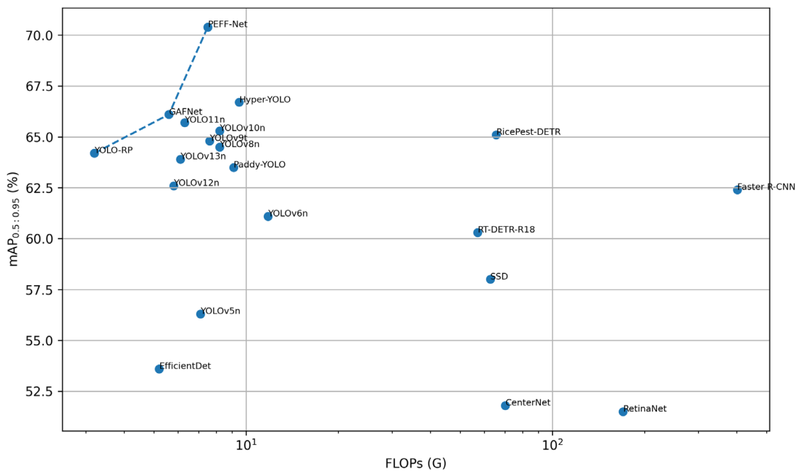
Figure 11 presents a Pareto-style comparison of detection accuracy and computational efficiency among the evaluated models. The horizontal axis represents FLOPs, while the vertical axis represents ${\mathrm{m}\mathrm{A}\mathrm{P}}_{0.5:0.95}$, and the dashed line indicates the Pareto frontier formed by the non-dominated models. PEFF-Net achieves the highest ${\mathrm{m}\mathrm{A}\mathrm{P}}_{0.5:0.95}$ among the evaluated models while maintaining a compact computational footprint with 2.12 M parameters and 7.5 G FLOPs. In comparison, some lightweight models, such as YOLO-RP and GAFNet, achieve lower computational costs but exhibit lower detection accuracy, whereas models with substantially higher computational complexity do not necessarily provide corresponding accuracy improvements. PEFF-Net is located on the Pareto frontier, demonstrating a favorable trade-off between detection accuracy and computational cost for edge-oriented rice pest detection applications.

3.3.6. Class-Wise and Scale-Wise Performance Analysis

To evaluate the detection performance of PEFF-Net across different pest categories and target scales, class-wise and scale-wise analyses were conducted on the Z-RP12 dataset. For comparison, YOLO11n was evaluated under the same conditions. The class-wise and scale-wise results are presented in

Table 12. Class-wise detection performance on the Z-RP12 dataset.

Pest Category	YOLO11n		PEFF-Net
	${\mathbf{A}\mathbf{P}}_{0.5}$ (%)	${\mathbf{A}\mathbf{P}}_{0.5:0.95}$ (%)	${\mathbf{A}\mathbf{P}}_{0.5}$ (%)	${\mathbf{A}\mathbf{P}}_{0.5:0.95}$ (%)
Rice stem fly	92.9	74.3	95.4	77.5
Asiatic rice borer	91.0	72.2	96.3	76.1
Rice plant hopper	82.7	60.0	86.3	65.9
Grain spreader thrips	79.6	55.4	89.2	62.3
Grub	87.8	66.7	92.4	70.2
Mole cricket	95.2	78.1	98.8	81.4
Paddy stem maggot	95.3	77.2	96.3	80.1
Rice gall midge	88.7	66.8	90.5	71.6
Rice leaf roller	60.3	37.1	66.2	46.2
Rice leaf hopper	73.5	51.5	83.8	57.9
Rice shell pest	93.2	74.6	95.1	77.4
Rice water weevil	93.6	74.9	96.4	78.8

and

Table 13. Scale-wise detection performance on the Z-RP12 dataset.

Model	${\mathbf{A}\mathbf{P}}_{\mathit{s}}$ (%)	${\mathbf{A}\mathbf{P}}_{\mathit{m}}$ (%)	${\mathbf{A}\mathbf{P}}_{\mathit{l}}$ (%)
YOLO11n	55.8	68.4	73.1
PEFF-Net	62.4	73.2	76.0

, respectively.

As shown in Table 12, PEFF-Net outperformed YOLO11n across all 12 pest categories in both ${\mathrm{A}\mathrm{P}}_{0.5}$ and ${\mathrm{A}\mathrm{P}}_{0.5:0.95}$. The largest AP0.5 improvements were observed for rice leaf hopper and grain spreader thrips, with gains of 10.3 and 9.6 percentage points, respectively. For AP0.5:0.95, the most pronounced improvements were obtained for rice leaf roller, grain spreader thrips, and rice leaf hopper, increasing by 9.1, 6.9, and 6.4 percentage points, respectively. These results indicate that PEFF-Net provides more consistent category-level detection and localization performance than YOLO11n, particularly for pest categories with relatively lower baseline performance.

To further evaluate the detection performance at different target scales, the test instances were categorized into small, medium, and large objects based on their bounding-box areas. The scale-wise results of YOLO11n and PEFF-Net are presented in Table 13.

As shown in Table 13, PEFF-Net achieved higher detection performance than YOLO11n across all three target scales. Specifically, AP_S, AP_M, and AP_L increased from 55.8%, 68.4%, and 73.1% to 62.4%, 73.2%, and 76.0%, corresponding to improvements of 6.6, 4.8, and 2.9 percentage points, respectively. The largest improvement was observed for small targets, indicating that PEFF-Net is particularly effective in detecting pest instances with limited spatial information. The larger gain for small targets is consistent with the design objective of PEFF-Net, where the high-resolution P2 branch and edge-aware feature processing are intended to preserve fine-grained spatial information for small-object detection.

Overall, the class-wise and scale-wise results demonstrate that PEFF-Net provides consistent improvements over YOLO11n across different pest categories and target sizes. In particular, the stronger gains for small targets further support the effectiveness of the proposed edge-aware feature extraction and cross-layer fusion strategy for small-pest detection.

4. Rice Pest Detection System

4.1. Overall System Architecture and Hardware Platform

4.1.1. Three-Tier Edge Deployment Framework

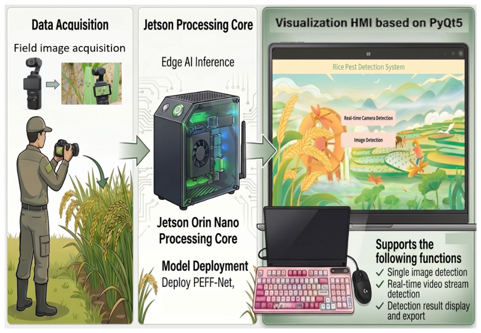
Figure 12 illustrates the overall architecture of the proposed edge-based pest detection system. Engineered to support real-time data collection and fully offline inference, this complete deployment framework directly couples the PEFF-Net model with Jetson Orin Nano Super 8 GB hardware and a PyQt5 visualization interface.

The system operates on a cohesive three-tier architecture, seamlessly integrating data acquisition, edge inference, and visualization to form a complete end-to-end diagnostic pipeline:

(1)

Data Acquisition Layer: Utilizing a handheld DJI Osmo Pocket 3 camera paired with a video capture card, this layer manages real-time field telemetry. Handheld operation allows for dynamic optical capture across diverse lighting conditions and viewing angles, while the capture card continuously streams this raw feed directly to the edge platform.

(2)

Edge Inference Layer: Anchored by the Jetson Orin Nano Super 8 GB, this core computational layer executes the PEFF-Net algorithm. It actively processes the incoming visual stream to extract pest classifications, spatial bounding boxes, and confidence scores. Hardware acceleration is fully leveraged to sustain real-time throughput without sacrificing diagnostic precision.

(3)

Visualization Interaction Layer: Rendered via the PyQt5 framework on a portable monitor, the user interface provides intuitive controls for static image analysis, live video monitoring, and data exportation. This streamlined interface empowers agricultural technicians to immediately assess and compile pest data directly in the field, drastically elevating overall system practicality.

4.1.2. System Hardware Components

The hardware components involved in this system are listed in

Table 14. System Hardware Components and Functions.

Hardware	Configuration	Function Description
Camera	DJI Osmo Pocket 3	Collects images and video streams of rice fields to provide raw input data for the detection system.
Edge computing platform	Jetson Orin Nano Super 8 GB	Deploys the PEFF-Net model and performs image preprocessing and object detection inference.
Protective enclosure	Yahboom Jetson mini case	Provides heat dissipation, physical protection, and portable mounting for the Jetson device.
Monitor	Yahboom 15.6-inch portable monitor	Displays detection results in real time and supports touch-based human–computer interaction.
Video capture card	MICHENSENT911	Captures and transmits video signals from the Osmo Pocket 3 to the Jetson platform in real time.

.

4.2. Data Acquisition Layer

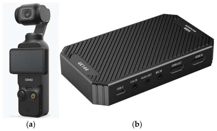
Figure 13 details the data acquisition hardware, coupling a DJI Osmo Pocket 3 camera with a MICHENSENT911 video capture card. This configuration directly streams real-time agricultural video feeds into the edge inference and visualization pipeline.

The DJI Osmo Pocket 3 was selected for its robust mechanical gimbal and excellent low-light adaptability. Capable of 1080P and 4K recording, it easily resolves minute pest details on rice leaves while neutralizing operator jitter during dynamic field capture. To bridge this optical sensor with the edge computing node, the MICHENSENT911 capture card converts HDMI outputs into USB streams. This hardwired transmission completely bypasses wireless network dependencies, guaranteeing reliable offline telemetry in remote agricultural settings. As mapped out in Figure 14, the overall acquisition workflow routes this raw feed directly to the Jetson edge device. Here, the incoming frames undergo strict preprocessing—including cropping and normalization to a 640 × 640 resolution—to furnish a standardized input stream for the PEFF-Net inference engine.

4.3. Edge Inference Layer

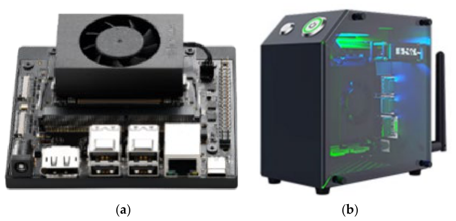
Operating as the computational core of the architecture, the edge inference layer translates raw optical inputs into actionable pest diagnostics entirely offline. As depicted in Figure 15, this localized processing is driven by a Jetson Orin Nano Super 8 GB platform housed within a Yahboom Jetson mini case. This dedicated hardware environment natively executes the PEFF-Net algorithm, seamlessly integrating inference acceleration and post-processing to maximize real-time throughput without relying on external cloud infrastructure.

To accommodate the strict power and computational constraints of edge deployment, we optimized PEFF-Net specifically for the Jetson Orin Nano Super 8 GB hardware. We first exported the native PyTorch model to the ONNX format, then utilized the TensorRT engine to execute layer fusion and INT8 quantization. This compilation process drastically compresses the memory footprint and computational overhead with negligible accuracy degradation. During active operation, this optimized engine ingests standardized images from the acquisition layer. Following forward inference, the system directly applies Non-Maximum Suppression to filter redundant bounding boxes, ultimately outputting precise pest classifications, spatial coordinates, and semantic confidence scores.

4.4. Visual Interactive Layer

Figure 16 details the visualization interaction layer, where a PyQt5 graphical interface is deployed on a Yahboom 15.6-inch portable monitor to provide field operators with direct, intuitive access to the real-time detection results.

The graphical interface features a streamlined modular layout, cleanly dividing operational controls from the primary visual display. The control panel equips operators with direct management over model selection, media ingestion, inference execution, and data exportation. Within the visual display, the system processes diagnostics through two distinct modes. In single-image mode, the framework evaluates localized uploads, instantly overlaying bounding boxes, taxonomic labels, and confidence thresholds onto the frame while aggregating pest counts. For dynamic field operation, the live video mode directly parses the continuous camera feed, superimposing real-time diagnostic metrics onto the moving frames to map pest distributions. All annotated visuals and aggregated statistics can be seamlessly exported, streamlining long-term agricultural tracking and traceability.

4.5. Deployment Performance Comparison on Jetson Edge Devices

To ensure a controlled edge-side comparison, YOLO11n and PEFF-Net were evaluated on the Jetson Orin Nano Super 8 GB using the same 640 × 640 input resolution, a batch size of 1, and deployment settings. Both models were additionally converted to TensorRT INT8 engines so that their edge-side performance could be compared under the same numerical precision. Both models were first exported to ONNX to evaluate numerical consistency between the original PyTorch models and exported models and were then converted to TensorRT INT8 engines for edge-side benchmarking under the same INT8 precision. Before timing, 50 warm-up iterations were executed and excluded from the reported statistics, followed by 200 measured inference iterations. CUDA synchronization was performed immediately before and after each timed inference call to avoid asynchronous execution bias. The device operated in the 25 W power-budget mode, with the CPU, GPU, and memory clocks fixed at their maximum available frequencies using jetson_clocks, and the stock cooling configuration was used without additional external cooling. Power consumption was measured using the on-board Jetson power-management integrated circuit (PMIC) and averaged over the benchmark interval. INT8 engines were calibrated using 200 representative images sampled exclusively from the training set, and no validation, test, or independent field images were used for calibration. Mean inference latency and FPS are summarized in

Table 15. Deployment performance comparison on the Jetson Orin Nano Super 8 GB.

Model	Optimization	${\mathbf{m}\mathbf{A}\mathbf{P}}_{0.5}$ (%)	Mean Latency (ms)	FPS
YOLO11n	PyTorch (.pt)	85.6	37.2	27
YOLO11n	ONNX	85.5	-	-
YOLO11n	TensorRT (INT8)	85.2	20.8	48
PEFF-Net	PyTorch (.pt)	90.1	62.5	16
PEFF-Net	ONNX	90.1	-	-
PEFF-Net	TensorRT (INT8)	89.7	32.1	31

Note: Latency was measured over the complete detector-processing pipeline, including preprocessing, data transfer, inference, bounding-box decoding, and NMS, while camera acquisition, disk I/O, and visualization were excluded. The reported latency and FPS values are averaged over 200 iterations after 50 warm-up runs under the 25 W power mode. ONNX results are provided for numerical-consistency verification, whereas latency comparisons are based on PyTorch and TensorRT implementations. The deployment results were obtained using the best checkpoint from the Seed 4 training run and evaluated directly on the Jetson Orin Nano Super 8 GB platform. The reported mAP values represent edge-device inference performance and may slightly differ from the desktop GPU evaluation results due to differences in hardware and inference runtimes.

, while latency percentiles, peak memory usage, and average power consumption are reported in

Table 16. Detailed INT8 Deployment Metrics of YOLO11n and PEFF-Net on the Jetson Orin Nano Super.

Model	Mean Latency (ms)	P50 (ms)	P95 (ms)	P99 (ms)	FPS	Peak Memory (MB)	Avg Power (W)
YOLO11n INT8	20.8	20.9	23.8	27.1	48	586	9.2
PEFF-Net INT8	32.1	31.5	35.8	41.2	31	812	10.5

.

Table 15 shows that the ONNX-exported models maintain comparable detection accuracy to the corresponding PyTorch checkpoints, with only a 0.1-percentage-point decrease in ${\mathrm{m}\mathrm{A}\mathrm{P}}_{0.5}$ for YOLO11n and no observable decrease for PEFF-Net. This indicates comparable numerical consistency between the PyTorch and ONNX implementations under the evaluated settings. After TensorRT INT8 conversion, YOLO11n decreases from 85.6% to 85.2% ${\mathrm{m}\mathrm{A}\mathrm{P}}_{0.5}$, while mean detector-pipeline latency decreases from 37.2 ms to 20.8 ms and throughput increases from 27 to 48 FPS. For PEFF-Net, ${\mathrm{m}\mathrm{A}\mathrm{P}}_{0.5}$ decreases from 90.1% to 89.7%, while mean latency decreases from 62.5 ms to 32.1 ms and throughput increases from 16 to 31 FPS. Under the same TensorRT INT8 precision, YOLO11n provides higher inference throughput, whereas PEFF-Net retains a 4.5-percentage-point advantage in ${\mathrm{m}\mathrm{A}\mathrm{P}}_{0.5}$. These results indicate that the export and quantization pipeline maintains comparable detection accuracy under the evaluated edge-deployment setting while providing substantial acceleration.

The INT8 latency statistics in Table 16 further characterize latency distribution and resource demand under the evaluated deployment conditions. YOLO11n INT8 records P50, P95, and P99 latencies of 20.9, 23.8, and 27.1 ms, respectively, with a peak memory usage of 586 MB and an average power consumption of 9.2 W. PEFF-Net INT8 records corresponding latencies of 31.5, 35.8, and 41.2 ms, with a peak memory usage of 812 MB and an average power consumption of 10.5 W. The higher latency and resource demand of PEFF-Net are consistent with its accuracy-oriented computational trade-off, while its 31 FPS throughput supports the real-time field pipeline evaluated in this study.

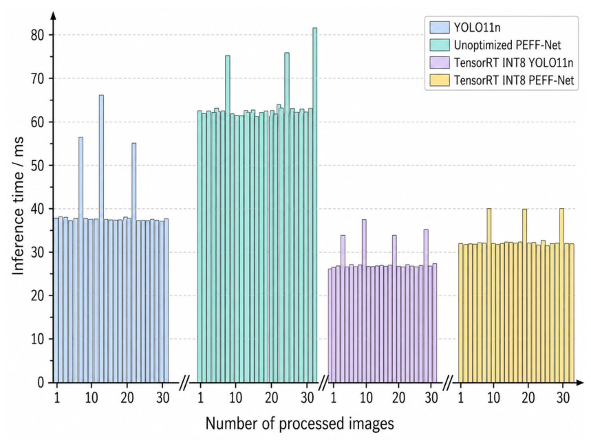
Figure 17 visualizes representative per-image inference latencies for four deployment configurations over the same 30-image sequence: YOLO11n in PyTorch, PEFF-Net in PyTorch, YOLO11n with TensorRT INT8, and PEFF-Net with TensorRT INT8. TensorRT acceleration reduces the latency of both models, with the representative INT8 traces concentrated around approximately 20–22 ms for YOLO11n and 31–33 ms for PEFF-Net. The 30-image sequence is used only to visualize per-image latency behavior; the percentile, memory, and power statistics in Table 16 are derived from the longer benchmark run described above. Consistent with Table 15, the same-precision comparison shows that YOLO11n INT8 is faster, whereas PEFF-Net INT8 retains higher detection accuracy.

4.6. Independent Field Evaluation and System Validation

To evaluate the performance of PEFF-Net on independently collected cross-camera field images, an independent dataset was collected in a paddy field in Qinghu Town, Jiangshan City, Zhejiang Province, China, using a DJI Osmo Pocket 3. The dataset comprised 200 images covering two rice pest categories, rice plant hopper and rice leaf roller, and was acquired during the middle and late rice growth stages under natural field conditions. Unlike the self-collected images in Z-RP12, which were captured using a HUAWEI Mate 70 Pro+, these images were collected independently and were completely separated from the training, validation, and test subsets of Z-RP12. They were not used for hyperparameter optimization or checkpoint selection. All images were manually annotated, and the final trained models were evaluated directly on this dataset without additional training or fine-tuning. The category-wise distribution of the independent field dataset is summarized in

Table 17. Distribution of the independent field test set.

Category	Images	Instances
Rice planthopper	87	93
Rice leaf roller	113	120
Total	200	213

.

To quantitatively evaluate detection performance under this cross-camera setting, YOLO11n and PEFF-Net were tested using the same inference settings. The results are presented in

Table 18. Detection performance on the independent field test set.

Model	P (%)	R (%)	${\mathbf{m}\mathbf{A}\mathbf{P}}_{0.5}$ (%)	${\mathbf{m}\mathbf{A}\mathbf{P}}_{0.5:0.95}$ (%)
YOLO11n	87.6	77.4	87.5	66.7
PEFF-Net	89.3	80.5	89.1	69.6

.

As shown in Table 18, PEFF-Net achieved a Precision of 89.3%, Recall of 80.5%, ${\mathrm{m}\mathrm{A}\mathrm{P}}_{0.5}$ of 89.1%, and ${\mathrm{m}\mathrm{A}\mathrm{P}}_{0.5:0.95}$ of 69.6% on the independent field test set. Compared with YOLO11n, PEFF-Net improved Precision, Recall, ${\mathrm{m}\mathrm{A}\mathrm{P}}_{0.5}$, and ${\mathrm{m}\mathrm{A}\mathrm{P}}_{0.5:0.95}$ by 1.7, 3.1, 1.6, and 2.9 percentage points, respectively. The consistent improvements across all four metrics indicate that the proposed feature-processing architecture remains effective on independently collected field images acquired using a camera different from that used for the self-collected component of Z-RP12. In particular, the 2.9-percentage-point improvement in ${\mathrm{m}\mathrm{A}\mathrm{P}}_{0.5:0.95}$ suggests improved localization performance under stricter IoU criteria.

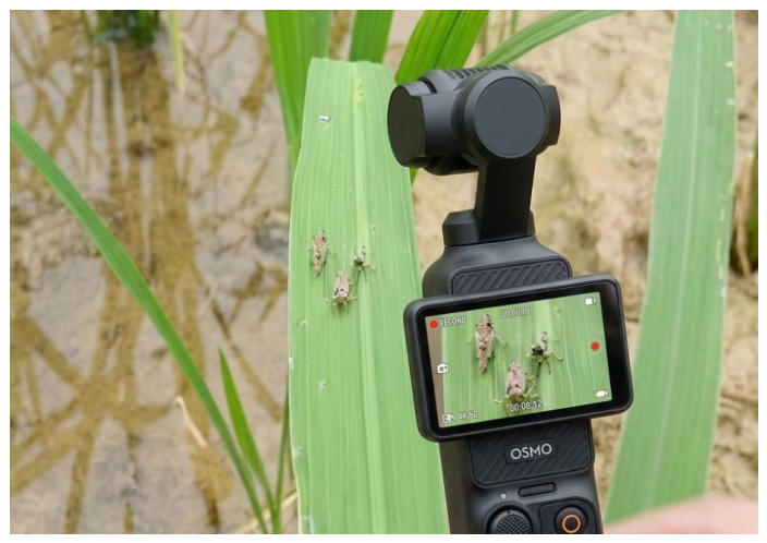
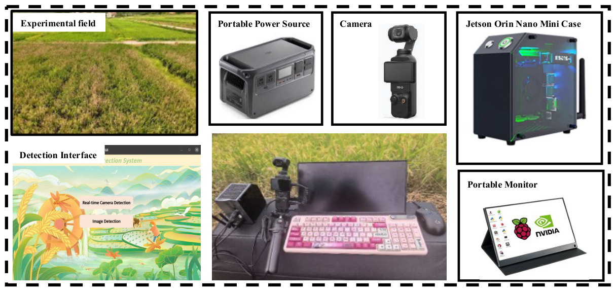
Following the quantitative independent evaluation, the complete rice pest detection system was further operated under actual field conditions to evaluate the feasibility of the camera–edge inference–visualization pipeline. Figure 18 shows the on-site deployment of the system during the field experiment.

During field operation, the Jetson Orin Nano Super 8 GB and portable monitor were powered on, and the detection program was launched through the graphical user interface. A DJI Osmo Pocket 3 was manually operated to capture rice plants and pest targets under natural field illumination. The camera output was transmitted through the HDMI video capture card and delivered to the Jetson Orin Nano Super 8 GB via a USB 3.0 interface. The incoming video stream was processed by the deployed PEFF-Net model, and the predicted pest categories, bounding boxes, and confidence scores were displayed synchronously on the portable monitor. This workflow enabled image acquisition, edge-side inference, and result visualization to be performed locally without relying on network connectivity.

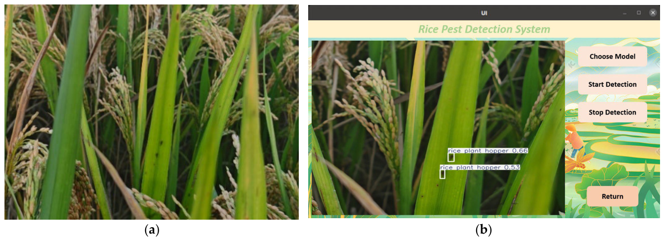
Representative detection results obtained during field operation are shown in Figure 19. Figure 19a presents an original field image, whereas Figure 19b shows the corresponding real-time detection result generated by the deployed system. The detected pest targets are displayed together with their predicted categories, bounding boxes, and confidence scores, illustrating the operation of the complete detection pipeline under practical field conditions.

Together with the deployment results in Section 4.5, the independent field evaluation demonstrates the feasibility of the proposed detection pipeline under the evaluated cross-camera field conditions. However, this validation is limited to two pest categories, one geographical area, and a relatively small number of annotated samples. Therefore, broader multi-location, multi-date, and annotated video evaluations are required to assess temporal stability and generalization across more diverse field environments.

5. Conclusions

This study developed the lightweight PEFF-Net detector and implemented an edge-side rice pest detection system on the Jetson Orin Nano Super 8 GB. Experimental results demonstrate that PEFF-Net achieves improved detection accuracy while maintaining a compact parameter footprint, while TensorRT INT8 acceleration enables real-time inference under the evaluated deployment configuration. The independent field test, consisting of 200 images and 213 instances from two pest categories acquired using a different camera, provides evidence of cross-camera feasibility under the specific field conditions examined in this study. However, the current validation is limited in pest categories, geographical coverage, acquisition dates, and temporal duration. Broader multi-location, multi-date, and annotated video evaluations will therefore be required to assess long-term robustness, temporal stability, and cross-location generalization.

Furthermore, this research is predominantly based on single-modal image data. In the future, we will focus on the fusion of multi-modal data, integrating multi-source information such as infrared images, hyperspectral data, and unmanned aerial vehicle (UAV) videos, to overcome the limitations of single-modal approaches concerning environmental adaptability and feature representation. Additionally, we will extend the model to multi-crop pest and disease detection and construct a multi-modal agricultural pest detection system. Concurrently, by integrating ecological models, we aim to assess farmland ecosystem health using pest detection data. For example, analysis of population dynamics between natural enemies and pests may provide data support for ecological pest management and sustainable agricultural practices.

References

1. FAO. World Food and Agriculture—Statistical Yearbook 2024; FAO: Rome, Italy, 2024. [Google Scholar]
2. Huang, M.-L.; Chuang, T.-C.; Liao, Y.-C. Application of transfer learning and image augmentation technology for tomato pest identification. Sustain. Comput. Inform. Syst. 2022, 33, 100646. [Google Scholar] [CrossRef] [Scilit]
3. Yang, J. Integrating big data analytics with hybrid machine learning approaches for precision agriculture and resource optimization. Sustain. Comput. Inform. Syst. 2026, 50, 101339. [Google Scholar] [CrossRef] [Scilit]
4. Kasinathan, T.; Uyyala, S.R. Machine learning ensemble with image processing for pest identification and classification in field crops. Neural Comput. Appl. 2021, 33, 7491–7504. [Google Scholar] [CrossRef] [Scilit]
5. Karadağ, K.; Tenekeci, M.E.; Taşaltın, R.; Bilgili, A. Detection of pepper fusarium disease using machine learning algorithms based on spectral reflectance. Sustain. Comput. Inform. Syst. 2020, 28, 100299. [Google Scholar] [CrossRef] [Scilit]
6. Vishwakarma, S.K.; Bhattarai, B.; Kothari, K.; Pandey, A. Intercomparison of machine learning models for estimating leaf area index of rice using UAV-based multispectral imagery. Phys. Chem. Earth Parts A/B/C 2025, 140, 103977. [Google Scholar] [CrossRef] [Scilit]
7. Gao, W.; Zong, C.; Wang, M.; Zhang, H.; Fang, Y. Intelligent identification of rice leaf disease based on YOLO V5-EFFICIENT. Crop Prot. 2024, 183, 106758. [Google Scholar] [CrossRef] [Scilit]
8. Zhu, L.; Li, X.; Sun, H.; Han, Y. Research on CBF-YOLO detection model for common soybean pests in complex environment. Comput. Electron. Agric. 2024, 216, 108515. [Google Scholar] [CrossRef] [Scilit]
9. Dai, Q.; Liang, S.; Li, Z.; Lyu, S.; Xue, X.; Song, S.; Huang, Y.; Zhang, S.; Fu, J. YOLOv11-RDTNet: A Lightweight Model for Citrus Pest and Disease Identification Based on an Improved YOLOv11n. Agronomy 2025, 15, 1252. [Google Scholar] [CrossRef] [Scilit]
10. Yang, X.; He, Q.; Xie, X.; Dong, M. YOLO-RP: A Lightweight and Efficient Detection Method for Small Rice Pests in Complex Field Environments. Symmetry 2025, 17, 1598. [Google Scholar] [CrossRef] [Scilit]
11. Zhou, Y.; Huang, W.; Liu, B.; Chen, T.; Wang, J.; Zhang, Q.; Yang, T. Lightweight GAFNet Model for Robust Rice Pest Detection in Complex Agricultural Environments. AgriEngineering 2026, 8, 26. [Google Scholar] [CrossRef] [Scilit]
12. Li, Z.; Li, Y. MCPDNet: Multi-scale feature fusion network for maize leaf disease and pest detection. J. Real-Time Image Process. 2026, 23, 72. [Google Scholar] [CrossRef] [Scilit]
13. Tang, Z.; Wang, Y.; Zou, D.; Qi, F. AEP-PEST: Adaptive edge-enhanced pyramid network for real-time detection of small and occluded agricultural pests. J. Real-Time Image Process. 2026, 23, 106. [Google Scholar] [CrossRef] [Scilit]
14. Xu, W.; Yang, R.; Karthikeyan, R.; Shi, Y.; Su, Q. GBiDC-PEST: A novel lightweight model for real-time multiclass tiny pest detection and mobile platform deployment. J. Integr. Agric. 2025, 24, 2749–2769. [Google Scholar] [CrossRef] [Scilit]
15. Wang, N.; Fu, S.; Rao, Q.; Zhang, G.; Ding, M. Insect-YOLO: A new method of crop insect detection. Comput. Electron. Agric. 2025, 232, 110085. [Google Scholar] [CrossRef] [Scilit]
16. Peng, Y.; Li, H.; Wu, P.; Zhang, Y.; Sun, X.; Wu, F. D-FINE: Redefine regression task of DETRs as fine-grained distribution refinement. In Proceedings of the International Conference on Learning Representations, Singapore, 24–28 April 2025. [Google Scholar]
17. Wu, X.; Zhan, C.; Lai, Y.; Cheng, M.; Yang, J. IP102: A Large-Scale Benchmark Dataset for Insect Pest Recognition. In Proceedings of the 2019 IEEE/CVF Conference on Computer Vision and Pattern Recognition (CVPR), Long Beach, CA, USA, 15–20 June 2019; pp. 8779–8788. [Google Scholar]
18. Ke, H.; Li, H.; Wang, B.; Tang, Q.; Lee, Y.; Yang, C. Integrations of LabelImg, You Only Look Once (YOLO), and Open Source Computer Vision Library (OpenCV) for Chicken Open Mouth Detection. Sens. Mater. 2024, 36, 4903–4913. [Google Scholar] [CrossRef] [Scilit]
19. Wang, W.; Dai, J.; Chen, Z.; Huang, Z.; Li, Z.; Zhu, X.; Hu, X.; Lu, T.; Lu, L.; Li, H.; et al. InternImage: Exploring large-scale vision foundation models with deformable convolutions. In Proceedings of the 2023 IEEE/CVF Conference on Computer Vision and Pattern Recognition (CVPR); IEEE: New York, NY, USA, 2023. [Google Scholar]
20. Selvaraju, R.R.; Cogswell, M.; Das, A.; Vedantam, R.; Parikh, D.; Batra, D. Grad-Cam: Visual explanations from deep networks via gradient-based localization. In Proceedings of the IEEE International Conference on Computer Vision, Venice, Italy, 22–29 October 2017. [Google Scholar]
21. Ma, X.; Dai, X.; Bai, Y.; Wang, Y.; Fu, F. Rewrite the Stars. In the Proceedings of the 2024 IEEE/CVF Conference on Computer Vision and Pattern Recognition (CVPR), Seattle, WA, USA, 16–22 June 2024; pp. 5694–5703. [Google Scholar]
22. Liu, X.; Peng, H.; Zheng, N.; Yang, Y.; Hu, H.; Yuan, Y. EfficientViT: Memory Efficient Vision Transformer with Cascaded Group Attention. In Proceedings of the 2023 IEEE/CVF Conference on Computer Vision and Pattern Recognition (CVPR), Vancouver, BC, Canada, 17–24 June 2023; pp. 14420–14430. [Google Scholar]
23. Chen, J.R.; Kao, S.-H.; He, H.; Zhuo, W.P.; Wen, S.; Lee, C.-H.; Chan, S.-H.G. Run, Don’t Walk: Chasing Higher FLOPS for Faster Neural Networks. In Proceedings of the 2023 IEEE/CVF Conference on Computer Vision and Pattern Recognition (CVPR), Vancouver, BC, Canada, 17–24 June 2023; pp. 12021–12031. [Google Scholar]
24. Qin, D.F.; Leichner, C.; Delakis, M.; Fornoni, M.; Luo, S.; Yang, F.; Wang, W.; Banbury, C.; Ye, C.; Akin, B.; et al. MobileNetV4: Universal Models for the Mobile Ecosystem. In Proceedings of the European Conference on Computer Vision—Eccv 2024, Pt XL; Springer: Cham, Switzerland, 2025; Volume 15098, pp. 78–96. [Google Scholar]
25. He, K.; Zhang, X.; Ren, S.; Sun, J. Deep residual learning for image recognition. In Proceedings of the IEEE Conference on Computer Vision and Pattern Recognition, Las Vegas, NV, USA, 27–30 June 2016. [Google Scholar]
26. Zhu, L.; Liao, B.; Zhang, Q.; Wang, X.; Liu, W.; Wang, X. Vision Mamba: Efficient Visual Representation Learning with Bidirectional State Space Model. In Proceedings of the International Conference on Machine Learning, Vienna, Austria, 21–27 July 2024. [Google Scholar]
27. Li, C.; Li, L.; Jiang, H.; Weng, K.; Geng, Y.; Li, L.; Ke, Z.; Li, Q.; Cheng, M.; Nie, W.; et al. YOLOv6: A Single-Stage Object Detection Framework for Industrial Applications. arXiv 2022, arXiv:2209.02976. [Google Scholar]
28. Wang, C.-Y.; Yeh, I.-H.; Liao, H.-Y.M. YOLOv9: Learning What You Want to Learn Using Programmable Gradient Information. In Computer Vision–ECCV 2024: 18th European Conference, Milan, Italy, September 29–October 4, 2024, Proceedings, Part XXXI; Springer: Milan, Italy, 2024; pp. 1–21. [Google Scholar]
29. Wang, A.; Chen, H.; Liu, L.; Chen, K.; Lin, Z.; Han, J.; Ding, G. Yolov10: Real-time end-to-end object detection. Adv. Neural Inf. Process. Syst. 2024, 37, 107984–108011. [Google Scholar] [CrossRef] [Scilit]
30. Tian, Y.; Ye, Q.; Doermann, D. YOLOv12: Attention-Centric Real-Time Object Detectors. arXiv 2025, arXiv:2502.12524. [Google Scholar]
31. Lei, M.; Li, S.; Wu, Y.; Hu, H.; Zhou, Y.; Zheng, X.; Ding, G.; Du, S.; Wu, Z.; Gao, Y. YOLOv13: Real-Time Object Detection with Hypergraph-Enhanced Adaptive Visual Perception. arXiv 2025, arXiv:2506.17733. [Google Scholar]
32. Feng, Y.; Huang, J.; Du, S.; Ying, S.; Yong, J.; Li, Y.; Ding, G.; Ji, R.; Gao, Y. Hyper-YOLO: When Visual Object Detection Meets Hypergraph Computation. IEEE Trans. Pattern Anal. Mach. Intell. 2024, 47, 2388–2401. [Google Scholar] [CrossRef] [Scilit] [PubMed]
33. Zhao, Y.; Lv, W.; Xu, S.; Wei, J.; Wang, G.; Dang, Q.; Liu, Y.; Chen, J. Detrs beat yolos on real-time object detection. In 2024 IEEE/CVF Conference on Computer Vision and Pattern Recognition (CVPR); IEEE: New York, NY, USA, 2024. [Google Scholar]
34. Ren, S.; He, K.; Girshick, R.; Sun, J. Faster R-CNN: Towards Real-Time Object Detection with Region Proposal Networks. IEEE Trans. Pattern Anal. Mach. Intell. 2017, 39, 1137–1149. [Google Scholar] [CrossRef] [Scilit] [PubMed]
35. Liu, W.; Anguelov, D.; Erhan, D.; Szegedy, C.; Szegedy, C.; Reed, S.; Fu, C.-Y.; Berg, A.C. SSD: Single Shot MultiBox Detector. In Computer Vision—ECCV 2016, Pt I; Springer Nature: London, UK, 2016; Volume 9905, pp. 21–37. [Google Scholar]
36. Lin, T.-Y.; Goyal, P.; Girshick, R.; He, K.; Dollár, P. Focal Loss for Dense Object Detection. In Proceedings of the 2017 IEEE International Conference on Computer Vision (ICCV), Venice, Italy, 22–29 October 2017; pp. 2999–3007. [Google Scholar]
37. Tan, M.; Pang, R.; Le, Q.V. EfficientDet: Scalable and efficient object detection. In Proceedings of the IEEE/CVF Conference on Computer Vision and Pattern Recognition, Seattle, DC, USA, 14–19 June 2020. [Google Scholar]
38. Duan, K.; Bai, S.; Xie, L.; Qi, H.; Huang, Q.; Tian, Q. Centernet: Keypoint triplets for object detection. In Proceedings of the IEEE/CVF International Conference on Computer Vision, Seoul, Republic of Korea, 27 October–2 November 2019. [Google Scholar]
39. Zheng, Y.; Zheng, W.; Du, X. Paddy-YOLO: An accurate method for rice pest detection. Comput. Electron. Agric. 2025, 238, 110777. [Google Scholar] [CrossRef] [Scilit]
40. Liu, J.; Zhou, C.; Zhu, Y.; Yang, B.; Liu, G.; Xiong, Y. RicePest-DETR: A transformer-based model for accurately identifying small rice pest by end-to-end detection mechanism. Comput. Electron. Agric. 2025, 235, 110373. [Google Scholar] [CrossRef] [Scilit]
Figure 1. Number of instances and distribution of bounding box. (a) the number of different kinds of instances in the dataset; (b) the distribution of target bounding boxes in the dataset; (c) the proportional distribution of target object centroids in the image; (d) the proportion of image space occupied by the target object.
Electronics 15 03836 g001
Figure 2. Examples of data augmentation images. (a) Original; (b) After small target clipping; (c) Horizontal flip; (d) Brightness adjustment; (e) Contrast adjustment; (f) Adding Gaussian Noise. The red frames indicate the locations of the target pests.
Electronics 15 03836 g002aElectronics 15 03836 g002b
Figure 3. Network architecture of PEFF-Net.
Electronics 15 03836 g003
Figure 4. Structure diagrams of different detection heads. (a) YOLO11n baseline structure; (b) YOLO11n-P2 structure; (c) YOLO-LCFO structure. Arrows indicate the feature transmission direction, and different colors represent different feature scales.
Electronics 15 03836 g004
Figure 5. Interactive interface of rice pest detection system.
Electronics 15 03836 g005
Figure 6. Functional interfaces of the rice pest detection system. (a) Real-time camera detection interface; (b) Single image detection interface.
Electronics 15 03836 g006aElectronics 15 03836 g006b
Figure 7. Grad-CAM Feature Visualization Comparison of Different Edge Detection Operators. The color intensity represents the feature activation level, with warmer colors indicating stronger responses.
Electronics 15 03836 g007
Figure 8. Trade-off between detection accuracy and inference speed with different backbone networks.
Electronics 15 03836 g008
Figure 9. Comparison of Rice Pest Detection Results with Different Neck Networks. The red dotted circles indicate pest targets that were missed by the detector.
Electronics 15 03836 g009
Figure 10. Feature maps and detection results of PEFF-Net and YOLO11n. (a) GT; (b) YOLO11n; (c) PEFF-Net; (d) Result. The green solid frames indicate ground-truth bounding boxes, the yellow dashed frames highlight the corresponding regions in the feature maps, and the blue frames with confidence scores represent predicted bounding boxes.
Electronics 15 03836 g010
Figure 11. FLOPs–accuracy Pareto comparison between PEFF-Net and mainstream object detection models. The dashed line represents the Pareto frontier formed by non-dominated models.
Electronics 15 03836 g011
Figure 12. Overall System Architecture.
Electronics 15 03836 g012
Figure 13. Hardware devices for data acquisition. (a) DJI Osmo Pocket 3 camera; (b) MICHENSENT911 video capture card.
Electronics 15 03836 g013
Figure 14. Field Image Acquisition Workflow for Rice Pest.
Electronics 15 03836 g014
Figure 15. Edge computing platform hardware. (a) Jetson Orin Nano Super 8 GB; (b) Yahboom Jetson mini case.
Electronics 15 03836 g015
Figure 16. Yahboom 15.6-inch portable monitor.
Electronics 15 03836 g016
Figure 17. Inference Time Comparison Between YOLO11n and PEFF-Net Under Different Deployment Methods on Jetson Edge Devices.
Electronics 15 03836 g017
Figure 18. On-site deployment test of the PEFF-Net model in the paddy field.
Electronics 15 03836 g018
Figure 19. Display of Real-time Detection Results. (a) Field original scene; (b) Real-time pest detection result on system interface.
Electronics 15 03836 g019