A Short-Term Electric Load Forecasting Method Integrating Grouped Exogenous Variable Recalibration and Calendar–Causal Dual Correction

Abstract

Short-term electric load forecasting is essential to the secure and stable operation and economic dispatch of power systems, and its accuracy directly affects grid dispatch decisions and operational efficiency. To address the inadequate modeling of heterogeneity among historical exogenous variables, the underutilization of known future calendar information, and the difficulty of correcting local biases in multi-step forecasts, this paper proposes KCD-GEIRTimeXer, a short-term electric load forecasting method built upon TimeXer. Before exogenous variable embedding, a Grouped Exogenous Importance Recalibration (GEIR) module is introduced. Historical exogenous variables are first grouped a priori according to their sources and physical meanings. Importance scores are then computed at the feature, variable-group, and time-step levels, and the corresponding exogenous variable weights are obtained through a bounded residual gating mechanism. At the prediction stage, a Known Calendar–Causal Dual Correction (KCD) module is further incorporated. The module refines the initial forecasts using known future calendar variables and causal statistical features derived exclusively from historical load observations, thereby mitigating local biases in multi-step forecasting. Experiments on the publicly available Panama electricity load dataset demonstrate that the proposed model outperforms all baseline models. Averaged over three random seeds, KCD-GEIRTimeXer reduces MSE, RMSE, MAE, and MAPE by 26.25%, 14.12%, 13.10%, and 12.91%, respectively, compared with TimeXer.

1. Introduction

In power system dispatch and electricity market operations, short-term electric load forecasting serves as a critical link between load variation patterns and operational decision-making, and its accuracy directly affects unit commitment, reserve capacity allocation, demand response, and electricity trading. Although observed as a univariate time series, load is jointly shaped by intraday and intraweek cycles, weather conditions, holidays, and user behavior. When the forecasting horizon spans peak-to-valley transitions, special dates, or abrupt weather changes, relying solely on superficial similarities among recent load patterns can lead to systematic forecasting biases. Early reviews and cross-regional comparisons have shown that sample organization, input selection, load periodicity, forecast horizon, and evaluation methodology can significantly affect model performance [1,2]. Therefore, accurate short-term load forecasting depends not merely on increasing model capacity, but on jointly modeling periodic priors, nonlinear fluctuations, and external drivers.

Traditional load forecasting approaches mainly rely on regression, exponential smoothing, and statistical time-series models, which generally require less data and offer strong interpretability. The semiparametric additive model developed by Fan and Hyndman [3] incorporated lagged loads, temperature trajectories, and calendar effects into a unified framework; related methods were subsequently extended to local load forecasting across large numbers of distribution substations [4]. Research on probabilistic load forecasting has further emphasized uncertainty representation, interval calibration, and evaluation rules [5]. Existing reviews have indicated that fixed functional forms struggle to adequately characterize the interactions among weather effects, behavioral changes, and multiple seasonal patterns. Moreover, low-voltage load forecasting is particularly sensitive to data granularity and record completeness [6,7]. A recent multidimensional study based on large-scale smart-meter data also revealed clear trade-offs among spatial aggregation levels, forecast horizons, peak-load errors, and computational costs [8]. These findings suggest that calendar and periodic priors remain valuable, but the relationships between exogenous variables and electric load require more flexible and dynamic representations.

With the development of deep learning, recurrent neural networks, residual architectures, and hybrid models have been widely used to capture nonlinear patterns and short- and long-term dependencies in load sequences. Studies using LSTM, including deep and pooling-enhanced architectures for residential load forecasting, have demonstrated the effectiveness of gated memory mechanisms in modeling temporal dependencies and inter-user heterogeneity [9,10,11]. Leon-Medina et al. [12] developed a GRU-based framework for high-resolution industrial energy-demand forecasting and demonstrated its advantages over LSTM and Conv1D models using quicklime-manufacturing data. Their study confirms the effectiveness of gated recurrent modeling for short-term demand forecasting, although it focuses on production-specific variables rather than the grouped heterogeneous weather and calendar information considered in this study. Feature selection, genetic-algorithm-based optimization, and residual connections have further improved input feature selection, hyperparameter optimization, and feature propagation [13,14]. Recent research has increasingly focused on hybrid networks, attention mechanisms, reinforcement learning, and multiscale representations. Across these studies, linear regression, CNN, BiGRU, DDPG, temporal convolution, and local–global interaction mechanisms have been incorporated in different ways to improve forecasting accuracy in complex scenarios [15,16,17,18,19]. However, most of these methods directly concatenate or uniformly encode exogenous variables, with limited explicit consideration of their sources, shared characteristics within variable groups, and sample-dependent contributions.

Transformer replaces recurrent computation with self-attention, providing a new approach to the parallel modeling of long-range dependencies [20]. For multi-step forecasting, existing studies have extended Transformer-based architectures by integrating known future covariates, sparse attention, series decomposition, and frequency-domain modeling [21,22,23,24]. Meanwhile, linear baselines, temporal patching, two-dimensional multi-period representations, and inverted variable tokens have prompted a reconsideration of how temporal structures and inter-variable dependencies should be modeled [25,26,27,28]. For forecasting tasks involving exogenous variables, Wang et al. [29] developed TimeXer, which bridges the target series and external information through patch-level self-attention over the endogenous series, variable-wise cross-attention, and a global endogenous token. This framework is closely aligned with the input setting considered in this study; however, it processes exogenous variables using a uniform embedding strategy and does not explicitly exploit known future calendar information available at the forecast origin. Recent studies published in 2026 have further explored recurrent and hybrid architectures for short-term load forecasting. Jiang and Xie [30] developed an improved bidirectional LSTM model for short-term load forecasting. Wang et al. [31] incorporated explicit weekly periodic features into a CNN–GRU and LightGBM hybrid model for short-term multi-step building load forecasting. Cao et al. [32] proposed a bidirectional GRU framework that integrates forecast-origin priors for multi-horizon load forecasting and power-system dispatch optimization. These studies demonstrate the effectiveness of recurrent modeling, periodic prior knowledge, and forecast-origin information. However, they do not jointly address source-aware recalibration of heterogeneous historical exogenous variables, known future calendar information, and bounded local bias correction within a unified framework.

Based on the above review and the task setting considered in this study, in which 168 h of historical information are used to directly forecast the load over the subsequent 24 h, existing methods still face three interrelated challenges. First, multi-site weather observations, aggregated meteorological indicators, and historical calendar variables differ substantially in their sources, physical meanings, and stability. A uniform embedding scheme therefore has difficulty representing the dynamic contribution of each variable to a given forecasting instance. Second, attributes within the forecast horizon—including the hour of day, day of week, month, weekend indicator, and holiday status—are known before forecasting begins. When relying solely on historical encodings, however, a model cannot explicitly distinguish the different temporal conditions associated with the 24 forecast steps. Third, although direct multi-step forecasting avoids recursive error propagation, local amplitude or phase deviations may still occur around peak-to-valley transitions, rapid load ramps, and periodic alignment points. Such deviations require bounded correction under strict information-availability constraints. More specifically, although TimeXer integrates exogenous information through cross-attention, it neither explicitly exploits source-based grouping before variable embedding nor provides a mechanism for bounded exogenous-variable recalibration at the feature, variable-group, and time-step levels. Its forecasting stage also lacks a dedicated step-wise correction branch for known future calendar attributes. Meanwhile, the final value of the historical window, recent load statistics, and daily and weekly periodic anchors are all available at the forecast origin, but they have not been systematically used to apply lightweight corrections to the base forecasts. Therefore, dynamically recalibrating heterogeneous exogenous variables, incorporating known future calendar information, and correcting local biases in multi-step forecasts—without introducing future ground-truth loads or future observed weather data—remains an important challenge.

To address the above challenges, this study proposes KCD-GEIRTimeXer, a method for short-term electric load forecasting. Built upon TimeXer, the proposed method introduces a Grouped Exogenous Importance Recalibration (GEIR) module before exogenous-variable embedding and incorporates a Known Calendar–Causal Dual Correction (KCD) module at the forecasting stage. GEIR groups exogenous variables a priori according to their sources and physical meanings and then performs multilevel, bounded, and sample-adaptive recalibration of historical exogenous information. KCD uses known future calendar variables available before forecasting begins and historical load statistics available before the forecast origin to apply bounded residual corrections to the base forecasts through two separate branches. In this study, the term “causal” indicates that all information used for correction strictly follows temporal ordering and the information-availability constraints at the forecast origin. It does not involve the identification of structural causal effects, nor does it use any future ground-truth values.

The main contributions of this study are summarized as follows:

• A Grouped Exogenous Importance Recalibration (GEIR) module is proposed. GEIR groups weather-station observations, aggregated meteorological indicators, and historical calendar information a priori according to their sources. It generates recalibration scores at the feature, variable-group, and time-step levels and employs an identity-centered bounded residual gate to constrain the magnitude of adjustment. This design enables exogenous-variable representations to adapt to sample-specific conditions while reducing the risk of excessive noise amplification.
• A Known Calendar–Causal Dual Correction (KCD) module is proposed. The known-calendar branch uses deterministic future information—including the hour of day, day of week, month, weekend indicator, and holiday status—to enrich the temporal semantics of each forecast step. The causally constrained branch uses only historical load statistics and periodic anchors available before the forecast origin to apply lightweight corrections to local amplitude and periodic deviations. Both branches adopt a bounded residual formulation, and neither future ground-truth loads nor future observed weather data are introduced during training or inference.
• A unified experimental protocol is established using the publicly available Panama hourly electric load dataset. GRU, LSTM, BiLSTM, Transformer, Informer, Autoformer, FEDformer, DLinear, PatchTST, and TimeXer are employed as baseline models. Overall performance evaluation, module ablation, representative load-scenario analysis, continuous forecasting, and input-perturbation experiments are conducted to systematically assess the individual contributions and combined effectiveness of GEIR and KCD, as well as the robustness of the proposed model.

2. Methodology

2.1. Problem Formulation

Let $y_t$ denote the electric load observed at hour t, and let ${\mathbf{X}}_t={[x_{t,1},x_{t,2},\dots ,x_{t,Z}]}^{\mathrm{T}}$ denote the corresponding historical exogenous-variable vector, where Z is the total number of historical exogenous variables. These variables include multi-station weather observations, aggregated meteorological indicators, and historical calendar features. According to their sources and physical meanings, the Z exogenous variables are divided into G predefined groups for subsequent importance recalibration. At each forecast origin t, the model uses a historical window of length L. The historical load sequence and the corresponding exogenous-variable matrix are expressed as

$$\left\{\begin{array}{cc}\hfill {\mathbf{y}}_t^{\mathrm{his}}& ={\left[y_{t-L+1},y_{t-L+2},\dots ,y_t\right]}^{\mathrm{T}}\hfill \\ \hfill {\mathbf{X}}_t^{\mathrm{his}}& ={\left[{\mathbf{X}}_{t-L+1},{\mathbf{X}}_{t-L+2},\dots ,{\mathbf{X}}_t\right]}^{\mathrm{T}}\hfill \end{array}\right.$$

(1)

In addition to the historical observations, calendar attributes within the forecast horizon are known at the forecast origin. Let ${\mathbf{c}}_{t+h}={[c_{t+h,1},c_{t+h,2},\dots ,c_{t+h,K}]}^{\mathrm{T}}$ denote the calendar-feature vector for the h-th forecast step, where K is the number of known future calendar features. These features include the hour of day, day of week, month, weekend indicator, and holiday status. The calendar information over the entire forecast horizon is represented as

$${\mathbf{C}}_t^{\mathrm{fut}}={[{\mathbf{c}}_{t+1},{\mathbf{c}}_{t+2},\dots ,{\mathbf{c}}_{t+H}]}^{\mathrm{T}}\in {\mathbb{R}}^{H\times K}.$$

(2)

The forecasting task is formulated as

$${\widehat{\mathbf{y}}}_t=F_{\mathit{\theta }}\left({\mathbf{y}}_t^{\mathrm{his}},{\mathbf{X}}_t^{\mathrm{his}},{\mathbf{C}}_t^{\mathrm{fut}}\right),$$

(3)

where $F_{\mathit{\theta }}(·)$ denotes the forecasting model parameterized by $\mathit{\theta }$, and ${\widehat{\mathbf{y}}}_t$ is the predicted load sequence. In this study, $L=168$ and $H=24$; therefore, the model uses information from the preceding 168 h to directly generate load forecasts for the subsequent 24 h in a single forward pass. To prevent information leakage, all model inputs must be available at the forecast origin. Historical load and exogenous observations are restricted to timestamps no later than t, whereas only deterministic calendar information known in advance is used within the future interval. Future ground-truth loads and future observed weather data are not used as model inputs during either training or inference.

2.2. Overall Architecture of KCD-GEIRTimeXer

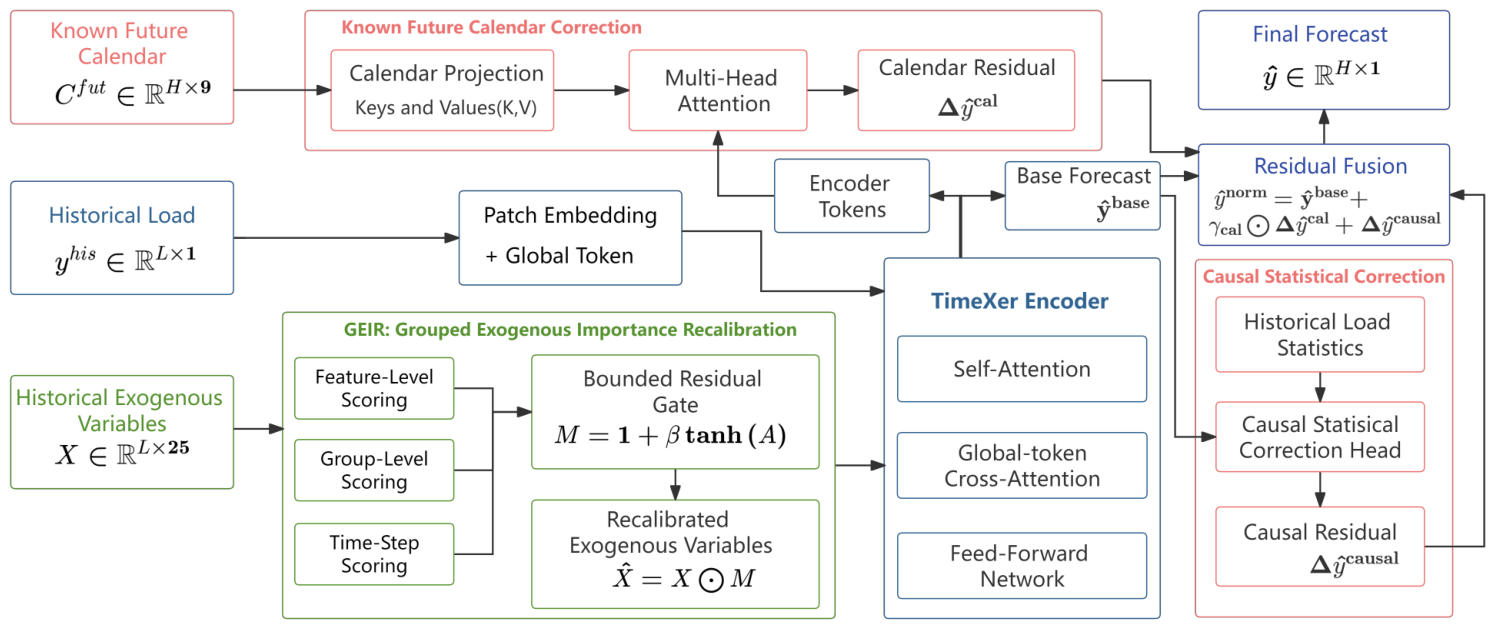
KCD-GEIRTimeXer consists of an input-side Grouped Exogenous Importance Recalibration (GEIR) module, a TimeXer encoder serving as the forecasting backbone, and an output-side Known Calendar–Causal Dual Correction (KCD) module. The overall architecture is illustrated in Figure 1. The model takes three types of inputs: the historical load sequence, historical exogenous variables, and known future calendar variables. The overall process comprises three stages: exogenous-variable recalibration, base-forecast generation, and dual-branch residual correction. First, the historical exogenous variables are fed into GEIR, which generates recalibration scores at the feature, group, and time-step levels. The three types of scores are fused and then passed through a bounded residual gate to constrain the magnitude of weight adjustment, producing the recalibrated exogenous variables $\widehat{\mathbf{X}}$. This operation is performed before exogenous-variable embedding, enabling the external information received by the forecasting backbone to reflect the relative importance of individual variables, variable groups, and historical time steps for the current forecasting instance. Subsequently, the historical load sequence is converted into load tokens through patch embedding, and a global endogenous token is appended. After embedding, the recalibrated exogenous variables and load tokens are jointly processed by the TimeXer encoder. The encoder employs self-attention to capture temporal dependencies among historical load patches, global-token cross-attention to establish interactions between the load representations and exogenous information, and a feed-forward network to further extract nonlinear features. This process produces the encoder tokens and the base forecasts for the subsequent 24 h.

Following base forecasting, KCD corrects the results from two complementary perspectives: known future calendar information and historical load statistics. The known-calendar correction branch first projects ${\mathbf{C}}^{\mathrm{fut}}$ into keys and values and uses the encoder tokens produced by TimeXer as queries. Multi-head attention is then applied to generate a calendar residual $\Delta {\widehat{\mathbf{y}}}^{\mathrm{cal}}$ corresponding to the temporal conditions of individual forecast steps. The causally constrained statistical correction branch extracts the final value of the historical window, recent load statistics, and daily and weekly periodic anchors and combines them with the base forecast to generate a causal correction residual $\Delta {\widehat{\mathbf{y}}}^{\mathrm{causal}}$. Finally, the residual-fusion unit combines the base forecast with the two correction residuals to produce the final forecast.

The placement of GEIR and KCD follows the information flow of the forecasting task rather than an arbitrary stacking of additional components. GEIR is applied before exogenous-variable embedding because it is designed to recalibrate heterogeneous historical external inputs before they are encoded by the forecasting backbone. In contrast, KCD is applied after base-forecast generation because it uses known future calendar information and historical load statistics to correct forecast-step-specific residual biases. TimeXer was selected as the backbone because its separate representations of endogenous and exogenous variables provide compatible interfaces for these two operations.

2.3. Grouped Exogenous Importance Recalibration Module

Historical weather observations, aggregated meteorological variables, and historical calendar variables differ in their semantic meanings and temporal dynamics. Moreover, their contributions to forecasting may vary with the state of the current historical window. To prevent a uniform embedding strategy from obscuring these differences, GEIR extracts state descriptors at the feature, variable-group, and time-step levels and adjusts the magnitude of exogenous-variable representations through bounded gating. Prior to model training, the variables are grouped a priori according to their sources, as shown in

Table 1. Prior grouping scheme for historical exogenous variables in GEIR.

Variable Group	Number of Variables	Description
G1: Station-Level Weather	12	Raw meteorological variables
G2: Aggregated Weather	4	Regionally aggregated meteorological variables
G3: Historical Calendar	9	Historical calendar variables

. Specifically, the 12 raw variables collected from three weather stations are assigned to the station-level weather group, four cross-station averaged features are assigned to the aggregated-weather group, and nine variables representing cyclic encodings and date-related states are assigned to the historical-calendar group.

2.3.1. Multilevel State Extraction and Scoring

Given the normalized historical exogenous-variable matrix $\mathbf{X}$, GEIR first constructs feature-level and group-level statistical descriptors. For each variable, the feature-level state consists of its mean, standard deviation, final value, and change between the first and final time steps within the historical window. The group-level state is constructed by extracting the corresponding statistics from the station-level weather, aggregated-weather, and historical-calendar groups:

$$\left\{\begin{array}{cc}\hfill {\mathbf{s}}^{\mathrm{f}}& =Concat\left[{Mean}_L\left(\mathbf{X}\right),{Std}_L\left(\mathbf{X}\right),{\mathbf{X}}_{L,:},{\mathbf{X}}_{L,:}-{\mathbf{X}}_{1,:}\right]\hfill \\ \hfill {\mathbf{s}}^{\mathrm{g}}& =GroupStat\left(\mathbf{X};\mathcal{G}\right)\hfill \end{array}\right.$$

(4)

where ${\mathbf{s}}^{\mathrm{f}}$ and ${\mathbf{s}}^{\mathrm{g}}$ denote the feature-level and group-level states, respectively, and $\mathcal{G}$ denotes the set of variable groups. $GroupStat(·)$ extracts the group mean, group standard deviation, mean value at the final time step, and mean change between the first and final time steps for each predefined variable group and then concatenates the statistics from all groups.

Based on the above statistical descriptors, GEIR generates recalibration scores at the feature, group, and time-step levels:

$$\left\{\begin{array}{cc}\hfill {\mathbf{a}}^{\mathrm{f}}& =F_f\left({\mathbf{s}}^{\mathrm{f}}\right)+{\lambda }_p{\mathit{\pi }}^{\mathrm{f}}\hfill \\ \hfill {\mathbf{a}}^{\mathrm{g}\to \mathrm{f}}& =Broadcast\left[F_g\left({\mathbf{s}}^{\mathrm{g}}\right)+{\lambda }_p{\mathit{\pi }}^{\mathrm{g}}\right]\hfill \\ \hfill {\mathbf{A}}^{\mathrm{t}}& =F_t\left(\mathbf{X}\right)\hfill \end{array}\right.$$

(5)

where $F_f(·)$, $F_g(·)$, and $F_t(·)$ denote the feature-level, group-level, and time-step-level scoring networks, respectively; ${\mathit{\pi }}^{\mathrm{f}}$ and ${\mathit{\pi }}^{\mathrm{g}}$ are learnable priors; and ${\lambda }_p$ is the prior scaling coefficient, which is set to 0.2 in this study. The group-level scoring network outputs three group scores corresponding to the station-level weather group, aggregated-weather group, and historical-calendar group. Each group score is subsequently broadcast to all variables belonging to the corresponding group, allowing variables within the same group to share a common group-level modulation signal. Variable-specific differences are further characterized by the feature-level scores.

2.3.2. Bounded Residual Recalibration

After the three types of scores are obtained, the feature-level and group-level scores are first combined through element-wise addition along the variable dimension. The resulting variable-level scores are then expanded across the historical time dimension and fused with the time-step-level scores:

$$\mathbf{A}={Expand}_L\left({\mathbf{a}}^{\mathrm{f}}+{\mathbf{a}}^{\mathrm{g}\to \mathrm{f}}\right)+\eta {\mathbf{A}}^{\mathrm{t}},$$

(6)

where ${Expand}_L(·)$ denotes the operation that replicates the variable-level scores across all L historical time steps, and $\eta$ is the scaling coefficient for the time-step-level scores, which is set to 0.5 in this study. Consequently, each element of the fused score incorporates the individual state of the corresponding variable, the shared state of its variable group, and the local state at the corresponding historical time step. To prevent unconstrained scores from excessively amplifying or suppressing certain exogenous variables, an identity-centered bounded residual gate is introduced to perform element-wise recalibration:

$$\left\{\begin{array}{cc}\hfill \mathbf{M}& =\mathbf{1}+\beta tanh\left(\mathbf{A}\right)\hfill \\ \hfill \widehat{\mathbf{X}}& =\mathbf{X}\odot \mathbf{M}\hfill \end{array}\right.$$

(7)

where $\mathbf{M}$ denotes the gating matrix, $\beta$ represents the maximum adjustment magnitude and is set to 0.5, and $\widehat{\mathbf{X}}$ denotes the recalibrated historical exogenous-variable matrix. Because the gating coefficients are bounded within $[0.5,1.5]$, GEIR does not directly eliminate any variable. Instead, it applies a limited degree of enhancement or suppression to different types of exogenous information. The output layers of the scoring networks are initialized to zero, allowing GEIR to approximate an identity mapping at the beginning of training and thereby reducing interference with the original representations used by TimeXer.

2.4. TimeXer-Based Forecasting Backbone

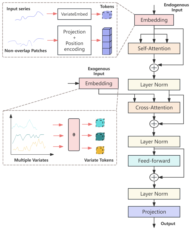
Existing Transformer-based models generally do not explicitly distinguish the different roles of endogenous and exogenous variables in time-series modeling. Instead, they often employ a unified embedding and attention-computation scheme, which may introduce redundant information and noise and consequently degrade forecasting accuracy [33]. TimeXer [29] is an enhanced Transformer architecture specifically designed for time-series forecasting with exogenous variables. The overall architecture of TimeXer is illustrated in Figure 2. Its core design employs differentiated embedding strategies and dual attention mechanisms to effectively distinguish and integrate the representations of endogenous and exogenous sequences.

TimeXer employs patch-wise and variable-wise embeddings to represent the endogenous load sequence and exogenous variables, respectively. The historical load sequence is first divided into N non-overlapping temporal patches $\{{\mathbf{s}}_1,{\mathbf{s}}_2,\dots ,{\mathbf{s}}_N\}$, each of which is mapped to an endogenous patch token. A learnable global token is also introduced to summarize the overall information of the endogenous sequence. In contrast, the complete historical trajectory of each exogenous variable is mapped to a variable-level token. The base forecasting process can be summarized as

$$\left\{\begin{array}{cc}\hfill \mathbf{P}& =PatchEmbed\left({\mathbf{s}}_1,{\mathbf{s}}_2,\dots ,{\mathbf{s}}_N\right)\hfill \\ \hfill \mathbf{V}& =VariateEmbed\left(\widehat{\mathbf{X}}\right)\hfill \\ \hfill \mathbf{h}& =Encoder\left(\mathbf{P},\mathbf{V}\right)\hfill \\ \hfill {\widehat{\mathbf{y}}}^{\mathrm{base}}& =Head\left(\mathbf{h}\right)\hfill \end{array}\right.$$

(8)

where $\mathbf{P}$ and $\mathbf{V}$ denote the endogenous patch tokens and exogenous variable tokens, respectively; $\mathbf{h}$ denotes the historical representation produced by TimeXer; and ${\widehat{\mathbf{y}}}^{\mathrm{base}}$ denotes the base forecast. The encoder first applies self-attention to model dependencies among different load patches. It then performs cross-attention using the global token as the query and the exogenous tokens as the keys and values, allowing historical exogenous information to be selectively incorporated into the load representation. Finally, the forecasting head uses the resulting representation to generate the base load forecasts.

2.5. Known Calendar–Causal Dual Correction Module

A Known Calendar–Causal Dual Correction module is constructed on top of the base forecasts produced by TimeXer. The module consists of a known future calendar attention branch and a causal multiscale statistical correction branch, which use deterministic future calendar information and historical load statistics, respectively, to generate forecast-step-specific corrections. Only information available at the forecast origin is used; neither future observed weather nor future ground-truth loads are involved in the computation. Here, the term “causal” only indicates that all statistical information is derived from load observations available at or before the forecast origin and does not refer to causal inference.

2.5.1. Known Future Calendar Correction

The historical encoded representation is first summarized through average pooling

$$\overline{\mathbf{h}}=MeanPool\left(\mathbf{h}\right),$$

(9)

and the resulting historical-state summary is replicated across the H future forecast steps and combined with forecast-step embeddings to construct the queries. Meanwhile, the deterministic future calendar variables are projected to form the keys and values used in the attention mechanism:

$$\left\{\begin{array}{cc}\hfill \mathbf{Q}& =F_q\left({Repeat}_H\left(\overline{\mathbf{h}}\right)\parallel {\mathbf{E}}^{\mathrm{hor}}\right)\hfill \\ \hfill {\mathbf{K}}^{\mathrm{cal}}& ={\mathbf{V}}^{\mathrm{cal}}=F_c\left({\mathbf{C}}^{\mathrm{fut}}\right)+{\mathbf{E}}^{\mathrm{hor}}\hfill \end{array}\right.$$

(10)

where ${\mathbf{E}}^{\mathrm{hor}}$ denotes the forecast-step embedding matrix, $\parallel$ denotes feature concatenation, and ${Repeat}_H(·)$ replicates the historical-state summary across all H forecast steps. $F_q(·)$ and $F_c(·)$ denote the query-projection and calendar-projection networks, respectively. The history-conditioned representations serve as the queries of multi-head attention, whereas the future calendar tokens serve as the keys and values. The calendar correction residual is then generated through a residual connection and a feed-forward network:

$$\left\{\begin{array}{cc}\hfill {\mathbf{A}}^{\mathrm{cal}}& =MHA\left(\mathbf{Q},{\mathbf{K}}^{\mathrm{cal}},{\mathbf{V}}^{\mathrm{cal}}\right)\hfill \\ \hfill {\mathbf{U}}^{\mathrm{cal}}& =\mathbf{Q}+{\rho }_{\mathrm{cal}}{\mathbf{A}}^{\mathrm{cal}}\hfill \\ \hfill \Delta {\widehat{\mathbf{y}}}^{\mathrm{cal}}& =F_{\mathrm{cal}}\left[{\mathbf{U}}^{\mathrm{cal}}+{\rho }_{\mathrm{cal}}FFN\left({\mathbf{U}}^{\mathrm{cal}}\right)\right]\hfill \end{array}\right.$$

(11)

where $MHA(·)$ and $FFN(·)$ denote the multi-head attention and feed-forward network, respectively. ${\rho }_{\mathrm{cal}}$ is the scaling coefficient of the calendar branch and is initialized to 0.1. Based on the current historical load state, this branch selectively extracts calendar information relevant to each forecast step, including the hour of day, day of week, weekend status, and holiday status. The output layer is initialized to zero so that the branch does not alter the base forecast at the beginning of training, while allowing it to progressively learn to compensate for future calendar effects during subsequent training.

2.5.2. Causally Constrained Multiscale Statistical Correction

The known future calendar correction provides calendar context for individual steps within the forecast horizon, but it cannot directly determine whether the base forecast deviates from recent load levels or daily and weekly periodic patterns. To further correct such local deviations, forecast-step-specific statistical features are constructed from the TimeXer base forecast and historical loads available before the forecast origin:

$${\mathbf{S}}^{\mathrm{causal}}={\mathsf{\Phi }}_{\mathrm{stat}}\left({\widehat{\mathbf{y}}}^{\mathrm{base}},{\tilde{\mathbf{y}}}^{\mathrm{his}}\right)\in {\mathbb{R}}^{H\times 11},$$

(12)

where ${\mathsf{\Phi }}_{\mathrm{stat}}(·)$ denotes the statistical-feature construction operation, which takes the historical load sequence and the base forecast as inputs. The resulting 11-dimensional feature vector comprises the base forecast, the load at the final time step of the historical window, the mean loads over the preceding 6, 24, and 168 h, the load changes over the preceding 6 and 24 h, daily and weekly periodic anchors, and the deviations between the base forecast and these periodic anchors. Except for the base forecast and its deviations from the periodic anchors, all statistical quantities are derived exclusively from historical loads available before the forecast origin. Therefore, this branch does not use future ground-truth loads.

The statistical features are subsequently encoded and fused with the forecast-step embeddings to generate amplitude-bounded, step-specific corrections:

$$\Delta {\widehat{\mathbf{y}}}^{\mathrm{causal}}={\rho }_s{r}_{max}tanh\left[F_o\left(F_s\left({\mathbf{S}}^{\mathrm{causal}}\right)+{\mathbf{E}}^{\mathrm{hor}}\right)\right],$$

(13)

where $F_s(·)$ and $F_o(·)$ denote the statistical-feature encoding network and the correction-output network, respectively. ${\rho }_s$ is the scaling coefficient of the statistical branch and is initialized to 0.1, whereas $r_{max}$ denotes the maximum residual range and is set to 0.5 in this study.

The feature-encoding network maps the 11-dimensional statistical features into the hidden space and adds them to the corresponding forecast-step embeddings. The correction-output network then generates the causal statistical correction terms. Their magnitudes are jointly controlled by the scaling coefficient and the maximum residual range, while $tanh(·)$ bounds the correction terms to prevent this branch from excessively altering the base forecast. This branch performs bounded residual compensation under temporal information-availability constraints rather than identifying causal relationships in the sense of causal inference.

2.5.3. Dual-Correction Fusion

The calendar and statistical corrections are both added to the base forecast in residual form, after which the load scale is restored through inverse instance normalization:

$$\left\{\begin{array}{cc}\hfill {\widehat{\mathbf{y}}}^{\mathrm{norm}}& ={\widehat{\mathbf{y}}}^{\mathrm{base}}+{\gamma }_{\mathrm{cal}}\odot \Delta {\widehat{\mathbf{y}}}^{\mathrm{cal}}+\Delta {\widehat{\mathbf{y}}}^{\mathrm{causal}}\hfill \\ \hfill \widehat{\mathbf{y}}& ={\sigma }_y{\widehat{\mathbf{y}}}^{\mathrm{norm}}+{\mu }_y\hfill \end{array}\right.$$

(14)

where ${\gamma }_{\mathrm{cal}}$ denotes a learnable calendar-output coefficient for each forecast step and is initialized to 1. ${\mu }_y$ and ${\sigma }_y$ denote the mean and standard deviation of the current historical load window, respectively, and $\widehat{\mathbf{y}}$ denotes the model output after inverse instance normalization. During evaluation, the original load units are further recovered using a target-variable scaler fitted exclusively on the training set.

The above fusion is not a weighted average of three independent predictors. Instead, the two correction branches provide complementary information regarding future temporal context and deviations from historical statistical patterns.

3. Experimental Setup

3.1. Dataset Description and Preprocessing

This study uses the publicly available Panama hourly electric load dataset. Experiments are conducted on hourly data processed under a strict no-information-leakage protocol. The processed dataset covers the period from 10 January 2015 to 27 June 2020 and contains 47,880 consecutive hourly observations. System load is used as the forecasting target, while the input variables include historical meteorological observations from three weather stations, cross-station aggregated meteorological variables, and calendar variables. The data are divided chronologically into training, validation, and test sets, accounting for 70%, 10%, and 20% of the observations, respectively.

The historical input length, forecast horizon, and dimensionality of the known future calendar variables are set to $L=168$, $H=24$, and $K=9$, respectively. These settings correspond to 168 h of historical input, load forecasting over the subsequent 24 h, and nine known future calendar variables. Electric load generally exhibits pronounced daily and weekly periodicities, while electricity consumption patterns differ between weekdays and weekends. Therefore, a 168 h historical window is adopted to cover seven consecutive days ($24\times 7=168$), thereby providing both intraday and intraweek periodic information.

The nine known future calendar variables comprise sine and cosine encodings of the hour of day, day of week, and month, together with indicators for weekends, holidays, and school days. These features are constructed from timestamps and predefined calendar records and are fully known at the forecast origin; therefore, they do not introduce future information leakage. The Panama dataset was selected because it provides a continuous hourly load series together with multi-site historical meteorological observations and calendar information, allowing the GEIR and KCD modules to be evaluated under a unified and reproducible protocol. The purpose of the present experiment is to provide a controlled methodological evaluation rather than a comprehensive cross-regional comparison.

3.2. Implementation Details

All experiments were conducted in Guilin, Guangxi, China, using a Windows-based workstation equipped with an Intel Core i5-13600KF processor and a Colorful GeForce RTX 4070 GPU. The software environment consisted of Python 3.9.25, PyTorch 2.0.0, and CUDA 11.8. The training and implementation settings of the proposed model are summarized in

Table 2. Common training hyperparameter settings for compared models.

Setting	Value
Historical input length L	168
Forecasting horizon H	24
Batch size	16
Optimizer	Adam
Initial learning rate	$1\times {10}^{-4}$
Learning-rate decay factor	0.5 per epoch
Maximum number of epochs	30
Early-stopping patience	5 epochs
Loss function	${\mathcal{L}}_{\mathrm{MSE}}$
Random seed	2024

. To avoid information leakage, all data-dependent preprocessing parameters, including the target-variable scaler, were fitted exclusively on the training set and subsequently applied to the validation and test sets.

All compared models were implemented within the same codebase and trained using a unified experimental protocol. No independent model-specific hyperparameter search was performed. The shared training hyperparameters were fixed consistently across all models, including the batch size, optimizer, initial learning rate, learning-rate schedule, maximum number of epochs, early-stopping criterion, MSE loss, and random seed. Model-specific structural operations were retained according to the corresponding model implementations, while the common architectural parameters were kept identical wherever applicable. For every model, the checkpoint with the lowest validation MSE was selected, and the test metrics were not used for hyperparameter tuning or checkpoint selection. The main architectural hyperparameters of the TimeXer forecasting backbone and the proposed GEIR and KCD modules are listed in

Table 3. Hyperparameter configuration of KCD-GEIRTimeXer.

Component	Hyperparameter	Symbol	Value
TimeXer	Model dimension	$d_{\mathrm{model}}$	256
TimeXer	Feed-forward dimension	$d_{\mathrm{ff}}$	512
TimeXer	Number of attention heads	—	8
TimeXer	Number of encoder layers	—	2
TimeXer	Patch length	—	24
TimeXer	Dropout rate	—	0.1
GEIR	Prior scaling coefficient	${\lambda }_p$	0.2
GEIR	Time-step score coefficient	$\eta$	0.5
GEIR	Maximum recalibration amplitude	$\beta$	0.5
KCD	calendar-branch scale	${\rho }_{\mathrm{cal}}$	0.1
KCD	calendar output coefficient	${\gamma }_{\mathrm{cal}}$	1.0
KCD	statistical-branch scale	${\rho }_s$	0.1
KCD	Maximum statistical residual	$r_{max}$	0.5

. These parameters were selected based on validation-set performance and kept fixed during testing.

Following Leon-Medina et al. [12], an adapted two-layer GRU baseline with 64 and 32 hidden units was implemented. Since the original study used 10-min industrial measurements and production-specific variables, only the forecasting architecture was transferred. Its input and output dimensions were adapted to the present 168-h-to-24-h forecasting task, and it was evaluated using the same chronological data split, preprocessing procedure, training loss, and evaluation metrics as the other baseline models. The output layers of the GEIR scoring networks and the two KCD correction branches were initialized to produce near-zero residual adjustments. Consequently, the proposed modules behave approximately as identity mappings at the beginning of training and gradually learn effective recalibration and correction patterns from the data. This initialization strategy reduces abrupt perturbations to the original TimeXer representations and improves training stability. The final model checkpoint was selected according to its performance on the validation set, and the test set was used only for the final evaluation.

3.3. Evaluation Metrics

This study employs Mean Squared Error (MSE), Root Mean Squared Error (RMSE), Mean Absolute Error (MAE), and Mean Absolute Percentage Error (MAPE) to evaluate model performance. Let M denote the total number of prediction points included in the test-set evaluation, and let $y_i$ and ${\widehat{y}}_i$ denote the actual and predicted loads at the i-th prediction point, respectively. The evaluation metrics are defined as follows:

$$\mathrm{MSE}={\displaystyle \frac{1}{M}}{\displaystyle \sum _{i=1}^M}{\left(y_i-{\widehat{y}}_i\right)}^2$$

(15)

$$\mathrm{RMSE}=\sqrt{{\displaystyle \frac{1}{M}}{\displaystyle \sum _{i=1}^M}{\left(y_i-{\widehat{y}}_i\right)}^2}$$

(16)

$$\mathrm{MAE}={\displaystyle \frac{1}{M}}{\displaystyle \sum _{i=1}^M}\left|y_i-{\widehat{y}}_i\right|$$

(17)

$$\mathrm{MAPE}={\displaystyle \frac{100\%}{M}}{\displaystyle \sum _{i=1}^M}\left|{\displaystyle \frac{y_i-{\widehat{y}}_i}{y_i}}\right|$$

(18)

4. Results and Discussion

4.1. Overall Performance Comparison

To evaluate the overall forecasting performance of the proposed model, ten representative methods, namely GRU, LSTM, BiLSTM, Transformer, Informer, Autoformer, FEDformer, DLinear, PatchTST, and TimeXer, were selected as benchmark models. These models cover recurrent neural networks, linear forecasting models, and various Transformer-based time-series forecasting architectures, thereby enabling a comprehensive evaluation of the proposed model across different modeling paradigms. To ensure a controlled comparison, all models were trained using the unified protocol described in Section 3.2, with the same dataset split, preprocessing procedure, look-back window, forecasting horizon, shared training hyperparameters, MSE loss, random seed, and evaluation procedure. During evaluation, the model outputs were sequentially transformed back through inverse instance normalization and the inverse transformation of the target-variable scaler. MSE, RMSE, MAE, and MAPE were subsequently calculated on the original load scale.

The quantitative forecasting results of the different models are presented in

Table 4. Experimental comparison of different models.

Model	MSE	RMSE	MAE	MAPE (%)
GRU	9344.55	96.67	70.56	5.910
Informer	8996.06	94.85	68.07	5.783
Transformer	8904.80	94.37	67.34	5.713
LSTM	8480.83	92.09	65.84	5.521
Autoformer	7741.47	87.99	63.21	5.353
BiLSTM	6898.50	83.06	60.49	5.084
FEDformer	6056.30	77.82	57.84	4.948
DLinear	5038.06	70.98	50.84	4.169
PatchTST	3824.35	61.84	44.70	3.742
TimeXer	3503.28	59.19	42.83	3.567
Proposed Model	2642.44	51.41	37.59	3.141

. The proposed model achieved the best performance across all four evaluation metrics, with MSE, RMSE, MAE, and MAPE values of 2642.44, 51.41, 37.59, and 3.141%, respectively. Compared with TimeXer, the proposed model reduced MSE, RMSE, MAE, and MAPE by 24.57%, 13.14%, 12.23%, and 11.94%, respectively. These relative improvements quantify the empirical gain over TimeXer under the adopted dataset and experimental protocol. They should not be interpreted as evidence that the forecasting error has reached its theoretical or empirical minimum. Nonzero forecasting errors remain in both the overall and scenario-specific evaluations, indicating that further improvements may still be possible. These results indicate that the incorporation of GEIR and KCD not only mitigates the contribution of large forecasting deviations to the overall error but also reduces both the average absolute error and the relative error. In particular, the 24.57% reduction in MSE demonstrates the stronger capability of the proposed model to suppress occasional large prediction errors.

Regarding the performance of different model categories, GRU, Informer, Transformer, and LSTM exhibited relatively large forecasting errors. The results indicate that the predictive performance of the GRU architecture reported for high-resolution industrial energy-demand forecasting does not directly transfer to hourly 24-step system-load forecasting. For the load-forecasting task considered in this study, conventional self-attention or recurrent architectures have difficulty simultaneously capturing periodic patterns, the effects of exogenous variables, and local fluctuations in the load sequence. Autoformer, BiLSTM, and FEDformer further improved forecasting performance through sequence decomposition, bidirectional temporal modeling, and frequency-domain representations, respectively. Nevertheless, their MAPE values remained between 4.948% and 5.353%. DLinear, PatchTST, and TimeXer achieved further improvements in forecasting accuracy. DLinear reduced the MAPE to 4.169%, indicating that the load series contains pronounced trend and periodic components and that linear decomposition models can provide a competitive forecasting baseline. By employing patch-based modeling, PatchTST improved the utilization of long historical input windows and further reduced the MAPE to 3.742%. TimeXer explicitly distinguishes the endogenous load series from historical exogenous variables and selectively incorporates exogenous information through cross-attention, achieving a MAPE of 3.567% and the best performance among all benchmark models. This result suggests that separately modeling endogenous and exogenous variables is advantageous for short-term load forecasting tasks involving meteorological and calendar information. Compared with PatchTST, KCD-GEIRTimeXer reduced MSE, RMSE, MAE, and MAPE by 30.90%, 16.87%, 15.91%, and 16.06%, respectively. Its further improvement over TimeXer also indicates that relying solely on cross-attention to integrate historical exogenous variables still has certain limitations.

To evaluate the robustness of the main forecasting results to random initialization and stochastic optimization, the comparison between TimeXer and KCD-GEIRTimeXer was repeated using three random seeds (2021, 2024, and 2026). All other experimental settings, including the dataset split, preprocessing procedure, model configuration, and training and evaluation protocols, were kept unchanged. The results are reported as the mean ± sample standard deviation in

Table 5. Multi-seed forecasting results.

Model	MSE	RMSE	MAE	MAPE (%)
TimeXer	$3562.15\pm 64.25$	$59.68\pm 0.54$	$43.04\pm 0.22$	$3.582\pm 0.014$
KCD-GEIRTimeXer	$2627.18\pm 34.16$	$51.26\pm 0.34$	$37.41\pm 0.16$	$3.120\pm 0.019$

. Across the three runs, KCD-GEIRTimeXer consistently outperformed TimeXer. Based on the mean results, it reduced MSE, RMSE, MAE, and MAPE by 26.25%, 14.12%, 13.10%, and 12.91%, respectively. The relatively small standard deviations indicate that the observed improvements are stable across the tested random seeds and are not driven solely by a favorable initialization.

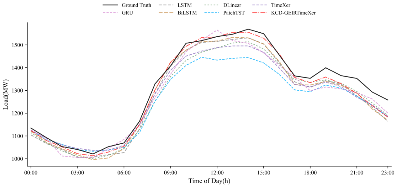
To provide a more intuitive comparison of the ability of different models to characterize intraday load variations, a complete weekday was selected from the test set for visualization, as shown in Figure 3. All models were able to capture the overall load pattern, including the overnight trough, the morning ramp-up, and the sustained high-load period in the afternoon. However, several benchmark models underestimated the rapid morning increase and the daytime peak load. In contrast, the predictions produced by KCD-GEIRTimeXer were closer to the actual load curve around the major turning points and during high-load periods. This result demonstrates that the proposed model provides improved tracking of local variations in multi-step load forecasting.

Overall, Table 4 and Figure 3 show that KCD-GEIRTimeXer achieves lower forecasting errors and more accurate intraday load tracking than the benchmark models. GEIR adaptively recalibrates historical exogenous variables, whereas KCD corrects local forecasting deviations using known future calendar information and historical load statistics. Their complementary input- and output-side enhancements improve the accuracy and stability of 24-h-ahead load forecasting.

4.2. Ablation Study

To assess the individual contributions of GEIR and KCD, three TimeXer-based variants were constructed: GEIRTimeXer, KCD-TimeXer, and KCD-GEIRTimeXer. All variants used the same dataset split, look-back window, forecasting horizon, training settings, and model-selection strategy. The ablation results are presented in

Table 6. Ablation results for the GEIR and KCD modules.

Model	MSE	RMSE	MAE	MAPE (%)
TimeXer	3503.28	59.19	42.83	3.567
GEIRTimeXer	3047.60	55.20	40.82	3.400
KCD-TimeXer	2666.28	51.63	38.05	3.178
KCD-GEIRTimeXer	2642.44	51.41	37.59	3.141

.

Both GEIR and KCD improve TimeXer when used independently. GEIRTimeXer reduces MSE, RMSE, MAE, and MAPE by 13.01%, 6.73%, 4.69%, and 4.68%, respectively, confirming the benefit of recalibrating historical exogenous inputs. KCD-TimeXer achieves larger reductions of 23.89%, 12.77%, 11.16%, and 10.91%, demonstrating the effectiveness of incorporating known future calendar information and historical load statistics at the forecasting stage. Combining both modules produces the lowest errors across all metrics.

Adding GEIR to KCD-TimeXer further reduces MSE, RMSE, MAE, and MAPE by 0.89%, 0.43%, 1.21%, and 1.16%, respectively. Although these incremental improvements are modest, they are consistently observed across all four evaluation metrics. As shown in Section 4.6, the number of trainable parameters increases from 2.871 M for KCD-TimeXer to 2.912 M for KCD-GEIRTimeXer, corresponding to only 40,913 additional parameters, or an increase of 1.42%. Therefore, GEIR provides a small but consistent improvement with limited additional parameter overhead. These results confirm that KCD is the primary source of the overall performance improvement, while GEIR provides a lightweight and complementary input-side enhancement. The purpose of this ablation study is to evaluate the contribution of each proposed module within the TimeXer-based framework, rather than to establish the global optimality of the overall architecture. The results demonstrate that GEIR and KCD independently improve the TimeXer backbone and that their combination achieves the lowest errors under the adopted experimental protocol. Therefore, the ablation results support the effectiveness and complementarity of the proposed modules within the investigated framework.

4.3. Forecasting Performance Under Different Load Scenarios

To evaluate the adaptability of KCD-GEIRTimeXer under different load conditions, the 9576 test observations were converted into 9553 rolling 24-h forecasting windows, corresponding to 229,272 forecast-origin–horizon pairs. Each pair represents a prediction made from a specific forecast origin for a specific forecast horizon. These pairs were assigned to three analytical subsets: regular load, weekend/holiday load, and high-volatility load.

The regular-load subset contains pairs whose target timestamps belong to neither the weekend/holiday subset nor the high-volatility subset. The weekend/holiday subset contains pairs whose target timestamps fall on weekends or holidays. A target point at time $\tau$ is classified as high-volatility when

$$\left|y_{\tau }-y_{\tau -1}\right|>q_{0.90}^{\mathrm{train}},$$

(19)

where $q_{0.90}^{\mathrm{train}}$ denotes the 90th percentile of the absolute one-hour load changes calculated exclusively from the training set. The weekend/holiday and high-volatility subsets are not mutually exclusive: 2192 forecast-origin–horizon pairs satisfy both definitions. Therefore, the numbers of evaluated pairs in the three subsets are not expected to sum to the total number of evaluated pairs. The corresponding results are presented in

Table 7. Scenario-wise performance comparison between TimeXer and KCD-GEIRTimeXer.

Load Scenario	Evaluated Pairs	Model	MSE	RMSE	MAE	MAPE (%)
Regular load	138,803	TimeXer	3391.11	58.23	42.54	3.438
		KCD-GEIRTimeXer	2841.37	53.30	38.46	3.136
Weekends and holidays	75,157	TimeXer	3712.58	60.93	43.45	3.872
		KCD-GEIRTimeXer	2467.43	49.67	36.93	3.243
High-volatility load	17,504	TimeXer	3579.89	59.83	43.33	3.345
		KCD-GEIRTimeXer	2564.09	50.64	36.13	2.814

.

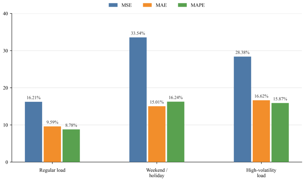
For each load scenario, TimeXer and KCD-GEIRTimeXer were evaluated using exactly the same forecast-origin–horizon pairs. The relative reduction in each metric was calculated using the TimeXer result as the reference, namely, by dividing the difference between the TimeXer error and the KCD-GEIRTimeXer error by the TimeXer error. Therefore, a positive reduction indicates that the proposed model achieves a lower forecasting error. These reductions represent empirical results for the defined test subsets rather than a theoretical guarantee for arbitrary datasets or operating conditions. KCD-GEIRTimeXer achieves lower errors across all scenarios and metrics. As illustrated in Figure 4, it reduces MSE, MAE, and MAPE by 16.21%, 9.59%, and 8.78% under regular conditions, respectively. The corresponding reductions are 33.54%, 15.01%, and 16.24% for weekends and holidays, and 28.38%, 16.62%, and 15.87% under high-volatility conditions. The comparatively smaller improvements under regular conditions may be explained by the relatively low baseline errors already achieved by TimeXer in this subset, leaving less scope for further correction. The larger improvements under weekends/holidays and high-volatility conditions indicate that the proposed modules are particularly beneficial under more complex load patterns.

Under relatively stable load conditions and regular calendar settings, the residual-correction mechanism of the proposed model remains effective in reducing forecasting errors. For weekends and holidays, the MSE and MAPE of TimeXer increase to 3712.58 and 3.872%, respectively, indicating that special calendar conditions increase forecasting difficulty. In contrast, the proposed model shows stronger adaptability to load-pattern changes associated with weekends and holidays. This finding is consistent with the intended role of the known-future calendar correction branch, which reduces errors in characterizing load levels and intraday patterns on special days. Under high-volatility conditions, the proposed model also effectively suppresses large forecasting deviations around rapid ramps, sharp declines, and local turning points.

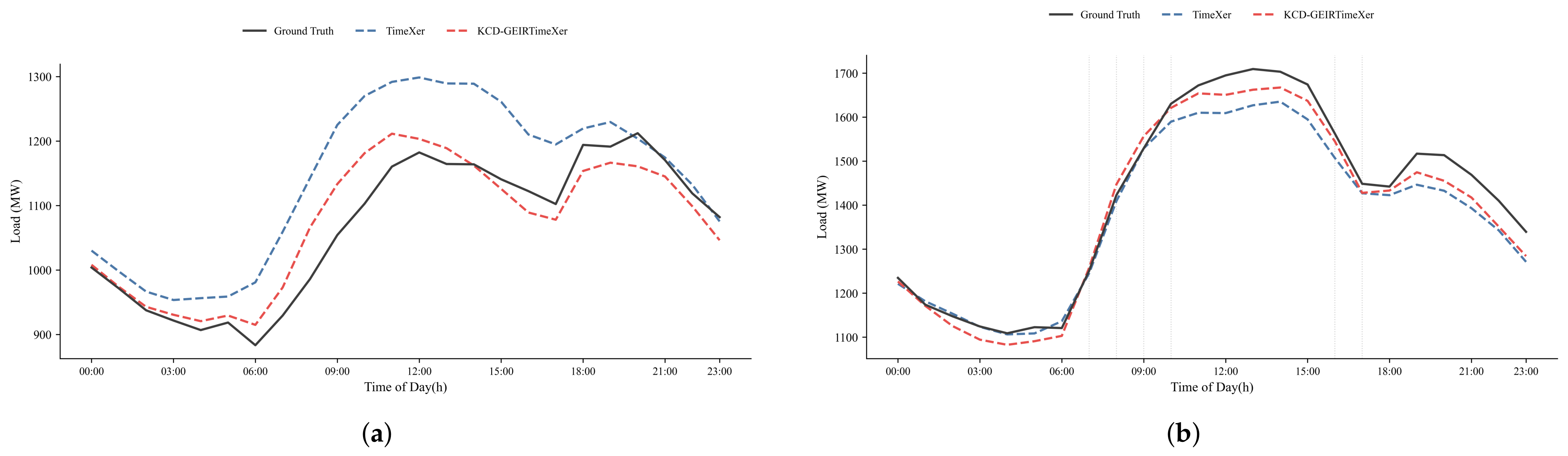
To further compare curve-tracking performance, representative holiday and high-volatility samples were selected from the test set. Figure 5 presents the corresponding 24-h forecasts produced by TimeXer and KCD-GEIRTimeXer.

In both scenarios, KCD-GEIRTimeXer more closely follows the actual load, particularly around peaks, ramps, and local turning points, supporting its improved adaptability to complex load conditions. From an operational perspective, more accurate 24-h load forecasts can support day-ahead unit-commitment and reserve-allocation decisions by improving estimates of load levels and peak timing. In particular, the improved performance on weekends and holidays may reduce scheduling mismatches caused by atypical daily patterns, while better tracking under high-volatility conditions may help operators schedule ramping reserves and demand-response resources around rapid load changes. These improvements may reduce the risks of overcommitment, insufficient reserves, and costly real-time balancing. However, because this study does not incorporate a unit-commitment, economic-dispatch, or electricity-market simulation, the associated economic and reliability benefits cannot yet be quantified.

4.4. Analysis of One-Week-Ahead Continuous Forecasting

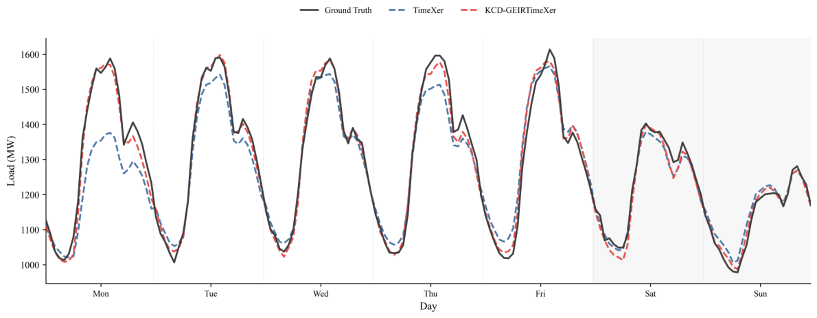
A single 24-h forecasting window can only reflect the model’s behavior over a local time period. To examine forecasting performance across multiple consecutive daily cycles, a complete calendar week without holidays was selected from the test set for qualitative analysis. Since the model generates a 24-h forecast at each run, Figure 6 was constructed by chronologically concatenating seven consecutive daily forecasting windows. Each window used the preceding 168 h of historical information. The gray shaded region denotes the weekend period, including Saturday and Sunday.

As shown in Figure 6, TimeXer captures the overall periodic trend of the weekly load but noticeably underestimates several weekday peaks. The proposed model more closely follows the actual load around major peaks, rapid declines, and post-trough recoveries. It also effectively tracks the transition from weekday to weekend load patterns, demonstrating more stable tracking of local load variations in continuous multi-day forecasting.

4.5. Robustness Analysis Under Meteorological Perturbations

To evaluate sensitivity to historical weather uncertainty, perturbation experiments were conducted on the trained TimeXer and KCD-GEIRTimeXer models without retraining. Perturbations were applied only to the 16 standardized historical meteorological variables, while load and calendar inputs remained unchanged. Gaussian noise with standard deviations of 0.05, 0.10, and 0.20 was added to these variables. Random missingness was simulated by independently setting weather inputs to zero with probabilities of 0.05, 0.10, and 0.20, where zero corresponds to the training-set mean in the standardized space. Each setting was evaluated using three random seeds (2024, 2025, and 2026), and the mean and standard deviation of MAPE were reported. The absolute MAPE shift was calculated relative to the unperturbed result, with lower values indicating lower sensitivity.

Table 8. MAPE and absolute MAPE shifts under different meteorological input perturbations.

Perturbation Type	Intensity	TimeXer MAPE (%)	KCD-GEIRTimeXer MAPE (%)	TimeXer Absolute MAPE Shift (%)	KCD-GEIRTimeXer Absolute MAPE Shift (%)
Gaussian Noise	$\alpha =0.05$	$3.5654\pm 0.0002$	$3.1412\pm 0.0012$	0.0468	0.0015
	$\alpha =0.10$	$3.5615\pm 0.0004$	$3.1413\pm 0.0022$	0.1574	0.0014
	$\alpha =0.20$	$3.5501\pm 0.0006$	$3.1437\pm 0.0041$	0.4764	0.0778
Random Missingness	$p=0.05$	$3.5488\pm 0.0017$	$3.1403\pm 0.0024$	0.5128	0.0297
	$p=0.10$	$3.5363\pm 0.0014$	$3.1439\pm 0.0031$	0.8618	0.0837
	$p=0.20$	$3.5217\pm 0.0017$	$3.1551\pm 0.0016$	1.2708	0.4420

presents the perturbation experiment results for the two models.

As shown in Table 8, KCD-GEIRTimeXer achieves a lower MAPE than TimeXer under all perturbation conditions. At the highest noise level of $\alpha =0.20$, the absolute MAPE shift of KCD-GEIRTimeXer is 83.67% lower than that of TimeXer, indicating that it is less sensitive to meteorological measurement noise. Random missingness has a greater overall impact on both models than Gaussian noise. Nevertheless, KCD-GEIRTimeXer maintains more stable forecasting performance. At $p=0.20$, its absolute MAPE shift is 65.22% lower than that of TimeXer. This indicates that the proposed model can maintain good forecasting accuracy even when a relatively high proportion of historical meteorological information is unavailable.

4.6. Computational Efficiency Analysis

To evaluate the computational burden introduced by GEIR and KCD, TimeXer and KCD-GEIRTimeXer were compared in terms of trainable parameters, estimated training time per epoch, inference latency per sample, and full-test-set inference time. All measurements were performed on an NVIDIA GeForce RTX 4070 GPU with a batch size of 16. Inference latency was averaged over 100 repetitions after 20 warm-up iterations, while the training-step time was averaged over 20 repetitions after five warm-up iterations and extrapolated to one training epoch. CUDA synchronization was applied before and after each timing operation. The results are presented in

Table 9. Computational efficiency comparison.

Model	Parameters (M)	Train/Epoch (s)	Inference/Sample (ms)	Test Time (s)
TimeXer	1.681	12.55	0.072	1.07
KCD-GEIRTimeXer	2.912	18.20	0.158	1.87

.

Compared with TimeXer, KCD-GEIRTimeXer increases the number of trainable parameters by 73.24%, the estimated training time per epoch by 44.98%, and the full-test-set inference time by 74.04%. Its per-sample inference latency is approximately 2.20 times that of TimeXer. Nevertheless, the absolute inference latency remains only 0.158 ms per sample, and the complete test set can be processed in approximately 1.87 s on the evaluated hardware. Therefore, although the proposed modules introduce additional computational overhead, the resulting latency remains small relative to the hourly sampling interval and the 24-h forecasting horizon.

The intermediate variants GEIRTimeXer and KCD-TimeXer contain 1.736 M and 2.871 M trainable parameters, respectively. GEIR alone increases the parameter count of TimeXer by only 3.29%, whereas KCD accounts for most of the additional model capacity. Moreover, adding GEIR to KCD-TimeXer increases the parameter count by only 1.42%. From a computational-complexity perspective, GEIR mainly introduces scoring operations that scale linearly with the historical input length and the number of exogenous variables, while KCD adds attention over the fixed forecasting horizon and lightweight statistical residual correction. These results indicate that the proposed model provides improved forecasting accuracy at the cost of a measurable but operationally manageable increase in computational demand.

4.7. Parameter Sensitivity Analysis

To examine whether the forecasting performance is strongly dependent on specific hyperparameter settings, a one-factor-at-a-time sensitivity analysis was conducted for six principal parameters: ${\lambda }_p$, $\eta$, $\beta$, ${\rho }_{\mathrm{cal}}$, ${\rho }_s$, and $r_{max}$. The default parameter configuration is listed in Table 3 and is reported only once in

Table 10. Parameter sensitivity results.

Varied Parameter	Value	MSE	RMSE	MAE	MAPE (%)
Default configuration	–	2642.44	51.41	37.59	3.141
${\lambda }_p$	0.10	2701.94	51.98	37.68	3.138
${\lambda }_p$	0.30	2712.52	52.08	37.77	3.146
$\eta$	0.25	2668.97	51.66	37.63	3.133
$\eta$	0.75	2723.90	52.19	37.78	3.148
$\beta$	0.25	2651.23	51.49	37.66	3.144
$\beta$	0.75	2721.77	52.17	37.75	3.142
${\rho }_{\mathrm{cal}}$	0.05	2661.67	51.59	37.56	3.128
${\rho }_{\mathrm{cal}}$	0.20	2705.84	52.02	37.67	3.137
${\rho }_s$	0.05	2680.86	51.78	37.61	3.131
${\rho }_s$	0.20	2707.42	52.03	37.79	3.146
$r_{max}$	0.25	2691.84	51.88	37.74	3.142
$r_{max}$	0.75	2715.80	52.11	37.72	3.142

to avoid repetition. In each sensitivity experiment, only the specified parameter was changed, while all remaining parameters were kept at their default values. All configurations were retrained using the same dataset split, training protocol, model-selection strategy, and random seed.

As shown in Table 10, the forecasting performance remains relatively stable across the tested parameter settings. Relative to the default configuration, the maximum deviations in MSE, RMSE, MAE, and MAPE are 3.08%, 1.52%, 0.52%, and 0.41%, respectively. The default configuration achieves the lowest MSE and RMSE while maintaining competitive MAE and MAPE values. Although setting ${\rho }_{\mathrm{cal}}$ to 0.05 slightly reduces MAE and MAPE, its MSE and RMSE remain higher than those of the default configuration, indicating a trade-off among different evaluation metrics rather than uniform superiority. The comparatively higher errors obtained at $\eta =0.75$ and $\beta =0.75$ suggest that overly strong time-step scoring or recalibration may introduce unnecessary perturbations to the historical exogenous representations. Overall, the limited variations across the tested ranges indicate that the proposed model is not strongly dependent on a narrowly specified hyperparameter configuration.

5. Conclusions

This study proposed KCD-GEIRTimeXer for 24-h short-term electricity load forecasting. The GEIR module adaptively recalibrates historical exogenous variables at the feature, variable-group, and time-step levels, reducing interference from redundant information and strengthening relevant meteorological and calendar representations. The KCD module further corrects the baseline forecasts using known future calendar information and multiscale statistical patterns derived from historical loads. Thus, the two modules enhance the forecasting process from the input and output sides, respectively.

Experiments on the Panama hourly electricity load dataset showed that KCD-GEIRTimeXer outperformed all benchmark models in the unified comparison. In the repeated comparison with TimeXer across three random seeds, the proposed model reduced the mean MSE, RMSE, MAE, and MAPE by 26.25%, 14.12%, 13.10%, and 12.91%, respectively, confirming that the observed improvement is not limited to a single favorable initialization. The ablation results confirmed that GEIR and KCD provide independent and complementary improvements. The proposed model also achieved consistent gains under regular-load, weekend/holiday, and high-volatility conditions, while more accurately tracking load variations over a continuous week. In addition, the meteorological perturbation experiments indicated lower sensitivity to noisy and missing weather inputs. However, the current evaluation is limited to a single regional dataset and a fixed 24-h forecasting horizon. Therefore, the findings should be interpreted within the evaluated dataset and forecasting setting. Future work will examine the model using geographically diverse datasets and different forecasting horizons, extend the framework to probabilistic load forecasting, and integrate the forecasting results with unit-commitment and reserve-allocation models to quantify their operational and economic benefits.

References

1. Hippert, H.S.; Pedreira, C.E.; Souza, R.C. Neural networks for short-term load forecasting: A review and evaluation. IEEE Trans. Power Syst. 2001, 16, 44–55. [Google Scholar] [CrossRef] [Scilit]
2. Taylor, J.W.; McSharry, P.E. Short-term load forecasting methods: An evaluation based on European data. IEEE Trans. Power Syst. 2007, 22, 2213–2219. [Google Scholar] [CrossRef] [Scilit]
3. Fan, S.; Hyndman, R.J. Short-term load forecasting based on a semi-parametric additive model. IEEE Trans. Power Syst. 2012, 27, 134–141. [Google Scholar] [CrossRef] [Scilit]
4. Goude, Y.; Nedellec, R.; Kong, N. Local short and middle term electricity load forecasting with semi-parametric additive models. IEEE Trans. Smart Grid 2014, 5, 440–446. [Google Scholar] [CrossRef] [Scilit]
5. Hong, T.; Fan, S. Probabilistic electric load forecasting: A tutorial review. Int. J. Forecast. 2016, 32, 914–938. [Google Scholar] [CrossRef] [Scilit]
6. Kuster, C.; Rezgui, Y.; Mourshed, M. Electrical load forecasting models: A critical systematic review. Sustain. Cities Soc. 2017, 35, 257–270. [Google Scholar] [CrossRef] [Scilit]
7. Haben, S.; Arora, S.; Giasemidis, G.; Voss, M.; Greetham, D.V. Review of low voltage load forecasting: Methods, applications, and recommendations. Appl. Energy 2021, 304, 117798. [Google Scholar] [CrossRef] [Scilit]
8. Li, H.; Heleno, M.; Zhang, W.; Sun, K.; Garcia, L.R.; Hong, T. A cross-dimensional analysis of data-driven short-term load forecasting methods with large-scale smart meter data. Energy Build. 2025, 344, 115909. [Google Scholar] [CrossRef] [Scilit]
9. Hochreiter, S.; Schmidhuber, J. Long short-term memory. Neural Comput. 1997, 9, 1735–1780. [Google Scholar] [CrossRef] [Scilit] [PubMed]
10. Shi, H.; Xu, M.; Li, R. Deep learning for household load forecasting—A novel pooling deep RNN. IEEE Trans. Smart Grid 2018, 9, 5271–5280. [Google Scholar] [CrossRef] [Scilit]
11. Kong, W.; Dong, Z.Y.; Hill, D.J.; Luo, F.; Xu, Y. Short-term residential load forecasting based on LSTM recurrent neural network. IEEE Trans. Smart Grid 2019, 10, 841–851. [Google Scholar] [CrossRef] [Scilit]
12. Leon-Medina, J.X.; Fonseca Gonzalez, J.E.; Callejas Rodriguez, N.Y.; González Niño, M.E.; Hernández Moreno, S.A.; Pineda-Munoz, W.A.; Siachoque Celys, C.P.; Umbarila Suarez, B.; Pozo, F. Forecasting Energy Demand in Quicklime Manufacturing: A Data-Driven Approach. Sensors 2025, 25, 7632. [Google Scholar] [CrossRef] [Scilit]
13. Bouktif, S.; Fiaz, A.; Ouni, A.; Serhani, M.A. Optimal deep learning LSTM model for electric load forecasting using feature selection and genetic algorithm: Comparison with machine learning approaches. Energies 2018, 11, 1636. [Google Scholar] [CrossRef] [Scilit]
14. Chen, K.; Chen, K.; Wang, Q.; He, Z.; Hu, J.; He, J. Short-term load forecasting with deep residual networks. IEEE Trans. Smart Grid 2019, 10, 3943–3952. [Google Scholar] [CrossRef] [Scilit]
15. Mohammed, F.; Boumaiza, A.; Sanfilippo, A.; Perez-Astudillo, D.; Bachour, D. A robust hybrid machine learning framework for short-term load forecasting: Integrating multi-linear regression, long short-term memory, and feed-forward neural networks for enhanced accuracy and efficiency. Energy AI 2025, 22, 100625. [Google Scholar] [CrossRef] [Scilit]
16. Ullah, K.; Akram, W.; Hassan, A.; Bokhari, S.A.S.; Abid, S.; Yousaf, H.; Farooq, A. Hybrid CNN–BiGRU model with attention mechanism for enhanced short-term load forecasting. Energy Rep. 2025, 14, 2570–2577. [Google Scholar] [CrossRef] [Scilit]
17. He, X.; Zhao, W.; Gao, Z.; Zhang, L.; Zhang, Q.; Li, X. A novel deep reinforcement learning model based on DDPG considering attention mechanism and combined with GRU network for short-term load forecasting. Appl. Soft Comput. 2025, 184, 113739. [Google Scholar] [CrossRef] [Scilit]
18. Mu, Y.; Kong, L.; Zheng, G.; Su, Z.; Wang, G. A short-term load forecasting method considering multiple feature factors based on long short-term memory and an improved temporal convolutional network. Eng. Appl. Artif. Intell. 2025, 159, 111649. [Google Scholar] [CrossRef] [Scilit]
19. Ding, X.; Li, D.; Luo, G.; Huang, W.; Chen, Y.; Zhang, Q.; Zhou, Q. MLGINet: An efficient network for short-term load forecasting based on multi-scale learning and local–global interactive learning. Neurocomputing 2025, 648, 130704. [Google Scholar] [CrossRef] [Scilit]
20. Vaswani, A.; Shazeer, N.; Parmar, N.; Uszkoreit, J.; Jones, L.; Gomez, A.N.; Kaiser, Ł.; Polosukhin, I. Attention is all you need. In Proceedings of the Advances in Neural Information Processing Systems, Long Beach, CA, USA, 4–9 December 2017; Volume 30, pp. 5998–6008. [Google Scholar]
21. Lim, B.; Arık, S.Ö.; Loeff, N.; Pfister, T. Temporal Fusion Transformers for interpretable multi-horizon time series forecasting. Int. J. Forecast. 2021, 37, 1748–1764. [Google Scholar] [CrossRef] [Scilit]
22. Zhou, H.; Zhang, S.; Peng, J.; Zhang, S.; Li, J.; Xiong, H.; Zhang, W. Informer: Beyond efficient transformer for long sequence time-series forecasting. In Proceedings of the AAAI Conference on Artificial Intelligence, Virtual, 2–9 February 2021; Volume 35, pp. 11106–11115. [Google Scholar] [CrossRef] [Scilit]
23. Wu, H.; Xu, J.; Wang, J.; Long, M. Autoformer: Decomposition transformers with auto-correlation for long-term series forecasting. In Proceedings of the Advances in Neural Information Processing Systems, Virtual, 6–14 December 2021; Volume 34, pp. 22419–22430. [Google Scholar]
24. Zhou, T.; Ma, Z.; Wen, Q.; Wang, X.; Sun, L.; Jin, R. FEDformer: Frequency enhanced decomposed transformer for long-term series forecasting. In Proceedings of the 39th International Conference on Machine Learning, Baltimore, MD, USA, 17–23 July 2022; Volume 162, pp. 27268–27286. [Google Scholar]
25. Zeng, A.; Chen, M.; Zhang, L.; Xu, Q. Are transformers effective for time series forecasting? In Proceedings of the AAAI Conference on Artificial Intelligence, Washington, DC, USA, 7–14 February 2023; Volume 37, pp. 11121–11128. [Google Scholar] [CrossRef] [Scilit]
26. Nie, Y.; Nguyen, N.H.; Sinthong, P.; Kalagnanam, J. A time series is worth 64 words: Long-term forecasting with transformers. In Proceedings of the International Conference on Learning Representations, Kigali, Rwanda, 1–5 May 2023. [Google Scholar]
27. Wu, H.; Hu, T.; Liu, Y.; Zhou, H.; Wang, J.; Long, M. TimesNet: Temporal 2D-variation modeling for general time series analysis. In Proceedings of the International Conference on Learning Representations, Kigali, Rwanda, 1–5 May 2023. [Google Scholar]
28. Liu, Y.; Hu, T.; Zhang, H.; Wu, H.; Wang, S.; Ma, L.; Long, M. iTransformer: Inverted transformers are effective for time series forecasting. In Proceedings of the International Conference on Learning Representations, Vienna, Austria, 7–11 May 2024. [Google Scholar]
29. Wang, Y.; Wu, H.; Dong, J.; Qin, G.; Zhang, H.; Liu, Y.; Qiu, Y.; Wang, J.; Long, M. TimeXer: Empowering transformers for time series forecasting with exogenous variables. In Proceedings of the Advances in Neural Information Processing Systems, Vancouver, BC, Canada, 10–15 December 2024; Volume 37, pp. 469–498. [Google Scholar] [CrossRef] [Scilit]
30. Jiang, W.; Xie, X. Short-term load forecasting based on the improved bi-directional long short-term memory model. Int. J. Electr. Power Energy Syst. 2026, 177, 111789. [Google Scholar] [CrossRef] [Scilit]
31. Wang, Z.; Chen, L.; Wang, C. Weekly periodicity feature-driven CNN-GRU and LightGBM hybrid model for short-term multi-step building load forecasting. Energy 2026, 355, 141163. [Google Scholar] [CrossRef] [Scilit]
32. Cao, F.; Zhang, J.-H.; Jia, G.-H. Multi-horizon short-term load forecasting for electric power system dispatch optimization: A bidirectional gated recurrent unit framework with forecast-origin prior integration and aligned evaluation. Processes 2026, 14, 2276. [Google Scholar] [CrossRef] [Scilit]
33. Li, J.; Zhang, B. Cloud workload prediction based on wavelet transform noise reduction and a TCN-GRU hybrid model. Cluster Comput. 2025, 28, 767. [Google Scholar] [CrossRef] [Scilit]
Figure 1. Overall architecture of the proposed KCD-GEIRTimeXer model.
Electronics 15 03825 g001
Figure 2. Overall architecture of the TimeXer model, adapted from Wang et al. [29].
Electronics 15 03825 g002
Figure 3. Comparison of forecasting curves from different models on a weekday.
Electronics 15 03825 g003
Figure 4. Relative error reductions under different load scenarios.
Electronics 15 03825 g004
Figure 5. (a) Holiday load scenario. (b) High-volatility load scenario.
Electronics 15 03825 g005
Figure 6. Comparison of actual and predicted load profiles over one continuous week.
Electronics 15 03825 g006