A Hybrid LHS–RSM Optimization Framework for Parameter Selection in Dielectric Gradient Topology Design

Abstract

Topology optimization has been widely applied to dielectric graded insulation design in gas-insulated switchgear (GIS); however, the selection of optimization parameters remains challenging due to strong coupling among design variables and the high computational cost of conventional parametric scanning methods. To address this issue, a hybrid optimization framework integrating Latin hypercube sampling (LHS) and response surface methodology (RSM) is proposed for efficient parameter selection in dielectric gradient topology design. The proposed framework combines global parameter space exploration, parameter space reduction, and multi-stage response surface optimization to construct surrogate models for efficient parameter optimization. The results show that the maximum electric field of the optimized insulator is reduced from 3.336 kV/mm to 1.400 kV/mm, demonstrating the effectiveness of the proposed method in improving electric field uniformity and optimization efficiency.

1. Introduction

Gas-Insulated Switchgear (GIS) is widely utilized in modern high-voltage power transmission and distribution systems due to its compact structure, high insulation reliability, and excellent operational performance. In GIS equipment, solid insulators play a crucial role in providing electrical insulation and mechanical support, and their electric field distribution directly determines the insulation performance of the system. However, due to the discontinuity of material properties and geometrical structures among electrodes, solid insulation, and gas media, electric field distortion frequently occurs, especially near the triple junction formed by the electrode, insulator, and gas medium. The resulting local electric field enhancement significantly reduces the insulation margin and may trigger partial discharge or surface flashover [1]. The accumulation of surface charges and the intrinsic trap states of dielectric materials are critical factors governing such electrostatic discharge behaviors across both high-voltage power equipment and aerospace applications [2]. Therefore, effective regulation of the electric field distribution inside and along the surface of insulators remains a key issue in the design of high-voltage insulation systems.

Functionally Graded Materials (FGMs) provide an effective approach for electric field regulation by introducing spatially varying dielectric properties within the insulation structure. Recently, the nonlinear electrical conduction and application of dielectric FGMs have been systematically reviewed as a highly effective approach for field grading in high-voltage applications [3]. By tailoring the permittivity distribution, the electric field can be redistributed without modifying the macroscopic geometry of the insulator. Early studies mainly focused on optimizing dielectric parameter distributions in graded insulation systems. Okubo et al. [4] proposed a bisection approximation algorithm based on Gauss’s law to optimize the permittivity distribution of coaxial d-FGM insulators. Kurimoto et al. [5] developed optimization strategies for d-FGM spacers by tailoring the permittivity distribution to alleviate the maximum surface electric field stress at the electrode interface. Various optimization methods have also been proposed to achieve optimal permittivity distributions in GIS spacers [6]. Later, topology optimization methods were introduced into dielectric gradient design. For instance, Lee et al. [7] applied topology shape optimization to dielectric materials, effectively alleviating the electric field intensity in high-voltage systems. Li et al. [8] further used topology optimization to construct dielectric gradient structures for suppressing electric field concentration. These studies demonstrate the feasibility of topology optimization for dielectric gradient insulation design.

However, existing optimization procedures still face challenges related to parameter selection and parameter coupling. In many studies, optimization parameters are determined through single-parameter scanning methods. However, traditional models for field calculation often suffer from high memory usage and long processing times, which severely limits the efficiency of insulator structural optimization [9]. Furthermore, while advanced metaheuristic algorithms, such as Genetic Algorithms (GA) [10,11] or Particle Swarm Optimization (PSO) [12], exhibit strong global search capabilities in high-voltage insulation design, they typically require thousands of iterative Finite Element Method (FEM) evaluations. In recent years, machine learning (ML) and deep learning techniques have been increasingly applied to the design of high-voltage engineering and GIS equipment [13], particularly for the rapid prediction of complex electric field distributions and the construction of advanced surrogate models for structural optimization [14,15]. Although these data-driven ML models exhibit exceptional predictive efficiency, their training process inherently relies on massive datasets. To overcome these limitations, Design of Experiments (DOE) provides a systematic framework for exploring the relationships between design variables and responses. For instance, Kim et al. [16] employed response surface methodology to optimize high-voltage insulator profiles, while Sima et al. [17] applied orthogonal experimental design to optimize the structural dimensions of converter valves. Therefore, integrating DOE-based strategies with topology optimization offers a promising solution for dielectric gradient insulation design.

In this paper, an efficient optimization framework combining topology optimization with DOE-based parameter exploration is proposed for dielectric gradient GIS insulators. First, Latin Hypercube Sampling (LHS) [18] is introduced to efficiently explore the global design space and identify promising parameter regions for dielectric gradient distribution, where the maximum relative permittivity is structurally constrained to 20 to ensure practical material synthesis feasibility. Second, a Response Surface Methodology (RSM) [19] based optimization strategy is established to construct surrogate models and refine the parameter optimization through multi-stage response surface analysis. Finally, an integrated LHS–RSM hybrid optimization framework is developed to achieve efficient parameter selection and optimization for dielectric gradient topology design. The proposed method significantly improves optimization efficiency while maintaining high accuracy in electric field regulation. Unlike metaheuristic algorithms that rely on repeated finite-element simulations, the proposed LHS–RSM framework constructs surrogate models to approximate the nonlinear relationships between design variables and the electric field response, significantly reducing the dependence on intensive FEM computations.

2. Topology Optimization Model of the Dielectric Graded Insulator

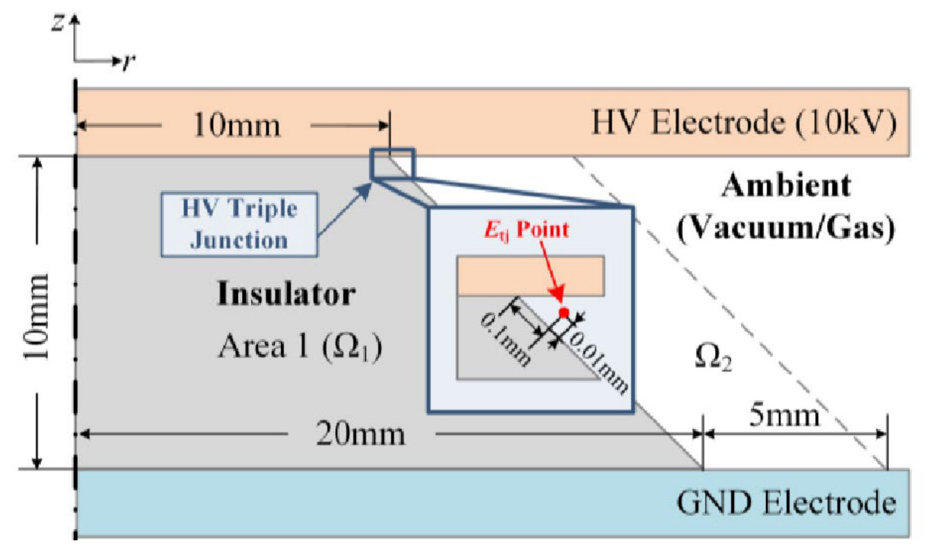
To optimize the electric field distribution of the insulator, the dielectric graded insulator topology optimization model proposed in previous studies is adopted as the research foundation in this work. The model considers a 45° conical insulator as the study object, as illustrated in Figure 1.

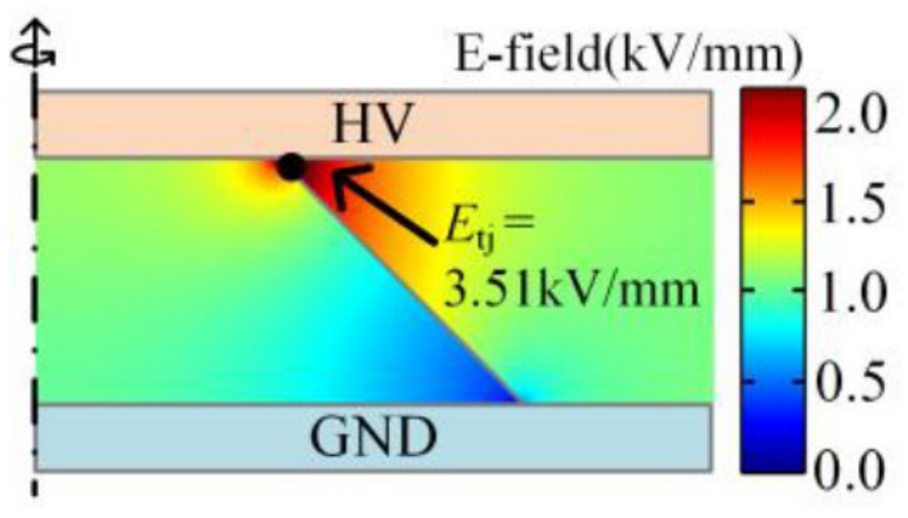
The electric field distribution of the conical insulator obtained from COMSOL Multiphysics 6.3 (COMSOL Inc., Burlington, MA, USA) simulation is shown in Figure 2. The color map represents the electric field magnitude, where warmer colors indicate higher electric field intensity. It can be observed that a strong electric field concentration appears near the triple-junction region between the high-voltage electrode, the insulator, and the gas medium. The maximum electric field at the triple junction reaches 3.51 kV/mm, which indicates a severe electric field distortion in this region. This phenomenon significantly reduces the insulation margin and may increase the risk of partial discharge or surface flashover. Under excessive local electric stress, electron-emission-induced ionization processes may further promote the initiation of localized discharge phenomena [20]. Therefore, effective regulation of the electric field distribution near the triple-junction region is essential for improving the insulation performance of GIS insulators.

By introducing a spatially varying permittivity distribution within the design domain of the insulator, the electric field distribution can be effectively regulated. The electric field is computed using the finite element method (FEM). To guarantee the reliability of the calculated electric field values, specific electrostatic boundary conditions were strictly defined in the FEM model, consistent with the base configuration established by Li et al. [8]. As illustrated in Figure 1, a Dirichlet boundary condition of 10 kV was applied to the high-voltage (HV) electrode, while the ground (GND) electrode was set to 0 V. The outer boundaries of the ambient gas domain were set as zero-charge (i.e., electric insulation, n × D = 0).

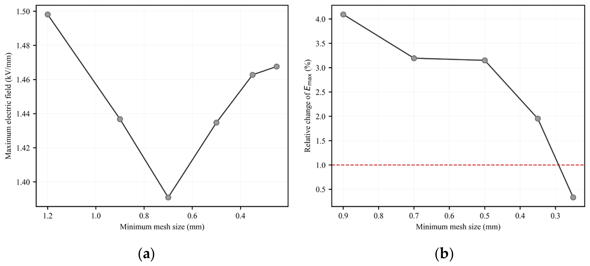
Furthermore, because the electric field at the triple junction is highly sensitive to grid density, a rigorous mesh independence study was conducted prior to the optimization. The local element size in the critical high-field region, denoted as h_mesh, was progressively refined from a coarse resolution of 1.2 mm down to a dense grid of 0.25 mm. As shown in Figure 3a, the calculated maximum electric field (E_max) gradually stabilizes as h_mesh decreases. Figure 3b further demonstrates that the relative variation in E_max drops to a negligible level once h_mesh is refined to 0.25 mm. To ensure absolute numerical stability during the subsequent topological iterations and accurate evaluation of the objective function, a local mesh size of h_mesh = 0.25 mm was ultimately adopted at the triple junction. This validation confirms that the calculated electric field values are mesh-independent and numerically stable.

In this model, the objective function consists of two components: the electric field uniformity index along the insulator surface and the electric field strength at the high-voltage triple-junction region. The mathematical formulation of the optimization problem is given as follows [8]:

$$\begin{gathered} \begin{array}{c}\mathrm{m}\mathrm{i}\mathrm{n}f={\int }_{\mathrm{Eopt}}+ q{f}_{\mathrm{grad}}\\ = w\left({\displaystyle \frac{1}{{\mathrm{C}}_{\mathrm{ref}}}}{\displaystyle {\int }_{{\mathsf{\Omega }}_2}}|E-E_{\mathrm{mean}}{|}^2\mathrm{d}\mathsf{\Omega }\right) + \left(1-w\right)\left({\displaystyle \frac{E_{\mathrm{tj}}}{E_{\mathrm{tj}0}}}\right)\\ +q{\displaystyle \frac{h_{\mathrm{mesh}}^2}{\mathrm{A}}}{\displaystyle {\int }_{{\mathsf{\Omega }}_1}}\left[{\left({\displaystyle \frac{\partial \rho }{\partial r}}\right)}^2+{\left({\displaystyle \frac{\partial \rho }{\partial z}}\right)}^2\right]\mathrm{d}\mathsf{\Omega }\end{array} \\ \mathrm{s}\text{.}\mathrm{t}\text{.}{\epsilon }_{\mathrm{r}}=\left({\epsilon }_{\mathit{rmax}}-{\epsilon }_{\mathit{rmin}}\right){\rho }_{\mathrm{i}}^p+{\epsilon }_{\mathit{rmin}}, p>0 \end{gathered}$$

(1)

The key parameters in the above model include the interpolation exponent p, the gradient penalty coefficient q, the objective function weighting factor w, and the upper bound of the relative permittivity ε_max. In practical insulation structures, the permittivity of the base material is usually determined by the intrinsic properties of the material itself, and its lower bound is essentially fixed. Therefore, in this study only the upper bound of the permittivity is treated as an optimization variable, while the lower bound is not optimized.

These parameters have a significant influence on the topology optimization results. Therefore, based on the above model, a systematic parameter optimization study is conducted in this work to determine the optimal parameter configuration.

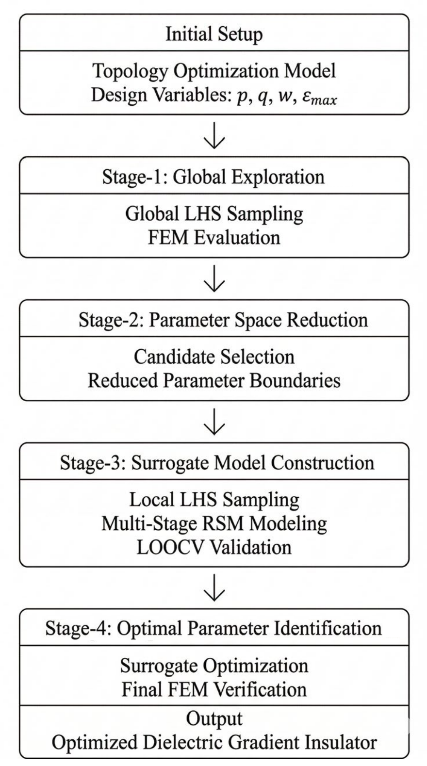
To systematically execute this, an integrated LHS–RSM hybrid optimization framework is proposed. The overall workflow of this methodological framework is intuitively illustrated in Figure 4. The procedure begins with the initial dielectric topology model. First, a global Design of Experiments (DOE) based on LHS is conducted to explore the macroscopic responses across the initial parameter space. Based on the evaluation of these samples, a mathematical sub-region determination is executed to narrow down the search space and isolate the most promising high-performance area. Subsequently, a robust surrogate model using RSM is constructed within this reduced subspace. Finally, the optimal parameter combination is pinpointed via the surrogate model, yielding the final optimized dielectric gradient structure. This integrated framework explicitly decouples the optimization iterations from exhaustive FEM simulations, thereby drastically reducing computational costs. The specific implementation of these phases will be detailed in the subsequent sections.

3. Parameter Optimization Based on Two-Stage Latin Hypercube Sampling

To obtain the optimal parameter configuration of the graded dielectric structure, it is necessary to explore a multidimensional design space to identify parameter combinations that can effectively improve electric field uniformity. Because the design variables are coupled with each other, conventional parametric scanning methods are computationally inefficient. Therefore, a two-stage Latin Hypercube Sampling (LHS) strategy is adopted for parameter optimization in this work.

The proposed approach first performs LHS in the global parameter space to identify promising regions, and then conducts a second LHS within a reduced parameter space around the promising region to further refine the optimal solution. Four key parameters are selected as optimization variables, including the shape parameters p and q, the gradient width w, and the maximum permittivity ε_max.

3.1. Global Exploration Using First-Stage LHS

The first stage aims to explore the global design space. The ranges of the design variables are listed in

Table 1. Parameter ranges used in the global LHS exploration.

Parameter	Description	Range
p	Interpolation exponent	0.6 ≤ p ≤ 1.4
q	Gradient penalty coefficient	6 ≤ q ≤ 20
w	Objective weighting factor	0.3 ≤ w ≤ 1.0
εmax	Maximum relative permittivity	10 ≤ εmax ≤ 30

.

To ensure the credibility and physical feasibility of the optimization process, the initial ranges for the four design variables listed in Table 1 were rigorously determined based on a combination of prior studies and preliminary simulations. Specifically, the ranges for the interpolation exponent (p in [0.6, 1.4]) and the gradient penalty coefficient (q in [6.0, 20.0]) were established encompassing the empirical values commonly utilized in classical variable density methods for dielectric design [8]. The weighting factor (w) was constrained within [0.3, 1.0] to ensure that the global electric field uniformity remains a dominant objective during the iteration. Furthermore, the upper bound of the relative permittivity was deliberately selected between 10 and 30 to reflect the practical manufacturing limits of current high-k functional composite materials (e.g., BaTiO₃/epoxy composites). This rational parameter bounding ensures that the LHS comprehensively covers the physically meaningful design space while preventing the FEM solver from encountering numerical divergence.

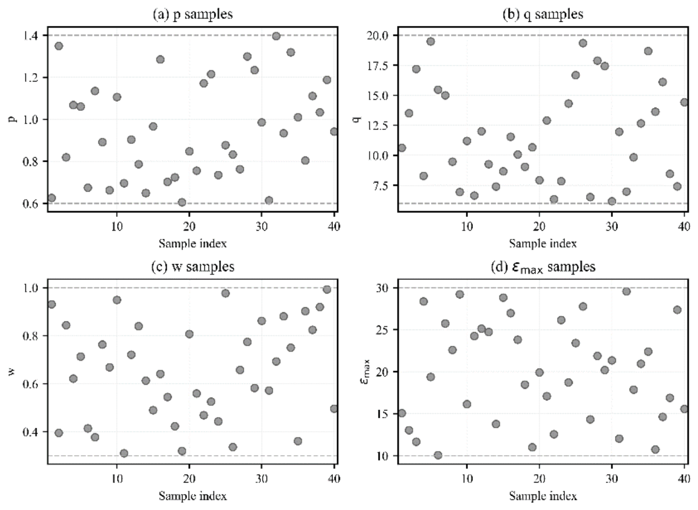
Within these explicitly defined ranges, the sample size for the initial global LHS was determined based on the widely adopted empirical “10$k$ rule” for computer experiments and surrogate modeling. This rule suggests that to achieve an optimal balance between multidimensional space-filling capacity and computational cost, the number of samples (N) should be approximately ten times the number of design variables (k). Given the four key design variables in this study (p, q, w, and ε_max, hence k = 4), the global sample size was set to N = 40. Consequently, 40 LHS samples were generated and evaluated using COMSOL simulations to obtain the corresponding objective values. The sampling distributions of the four parameters are illustrated in Figure 5. It can be observed that the samples are evenly distributed across the parameter ranges without significant clustering or gaps. This indicates that the selected sample size and the LHS approach effectively cover the multidimensional design space with sufficient resolution, successfully capturing macroscopic nonlinear relationships without incurring unnecessary FEM computational burden.

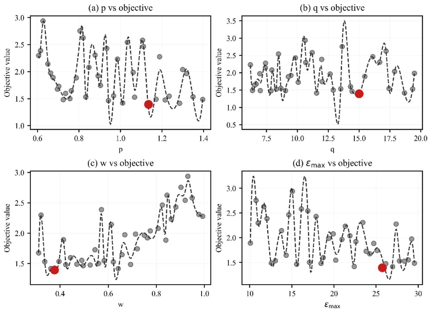
To further investigate the influence of each parameter on the objective function, the relationships between the design variables and the objective values are presented in Figure 6. The gray points represent the sampled solutions, the dashed curves indicate the trends derived from the data, and the red markers denote the best solution obtained from the first-stage search.

From these results, it can be observed that the parameters exhibit different levels of influence on the objective function. Parameter p tends to produce lower objective values at moderately large values, while q shows favorable performance within a middle range. The parameter w achieves better results at relatively small values, suggesting that a narrow gradient region is beneficial for electric field homogenization. In addition, larger values of ε_max generally contribute to reducing the electric field non-uniformity.

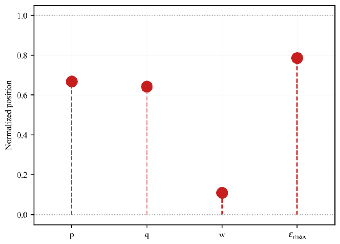
The normalized positions of the optimal parameters obtained in the first stage are presented in Figure 7. It can be observed that the optimal value of w lies close to its lower bound, while the other parameters are located in the middle regions of their ranges. This indicates that a relatively small gradient width may be beneficial for improving the electric field uniformity. However, since this stage mainly performs global exploration, the obtained solution only indicates a promising region.

3.2. Local Refinement Using Second-Stage LHS

To ensure reproducibility and methodological rigor, the boundaries of the reduced parameter space in the second stage were established using a threshold-based hyper-rectangular bounding criterion. Specifically, a high-performance subset was extracted from the first-stage global LHS, defined by samples whose objective values were lower than the median of the initial population (i.e., $f_{\mathrm{obj}}\le f_{\mathrm{median}}$). The secondary search boundaries were then mathematically determined by calculating the minimum and maximum coordinates of this subset for each parameter, denoted as $x_{i,\mathit{sub}}^{\mathit{min}}$ and $x_{i,\mathit{sub}}^{\mathit{max}}$. To avoid premature exclusion of the global optimum at the parameter edges, a 5% relaxation margin (α = 0.05) relative to the initial global parameter range (Δx_i) was introduced. The refined boundaries were defined by the equations:

$$\begin{array}{rr}& x_{i,\mathit{new}}^{\mathit{min}}=\mathit{max}\left(x_i^{\mathit{global},\mathit{min}},\hspace{0.17em}{x}_{i,\mathit{sub}}^{\mathit{min}}-\alpha \Delta x_i\right)\\ & x_{i,\mathit{new}}^{\mathit{max}}=\mathit{min}\left(x_i^{\mathit{global},\mathit{max}},\hspace{0.17em}{x}_{i,\mathit{sub}}^{\mathit{max}}+\alpha \Delta x_i\right)\end{array}$$

(2)

This mathematical criterion successfully truncated the underperforming sub-regions (e.g., strictly narrowing parameter w to [0.328, 0.60] and p to [0.651, 1.40]) while preserving the full exploration range for parameters that maintained favorable responses across their global domain (such as parameter q). The resulting secondary sampling ranges for the parameters are listed in

Table 2. Parameter ranges used in the second-stage LHS.

Parameter	Secondary Sampling Ranges
p	0.651–1.40
q	6.0–20.0
w	0.328–0.60
εmax	10.86–30.0

.

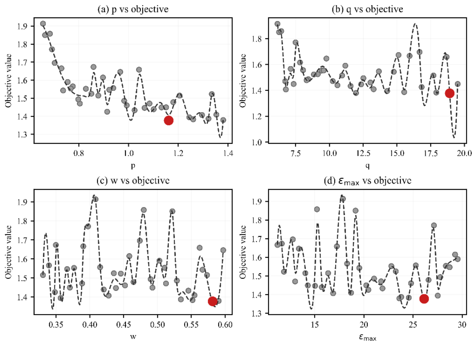
The relationships between the parameters and the objective values obtained in the second stage are shown in Figure 8. Compared with the first stage, the objective values are generally lower and the variation trend becomes clearer, indicating that the local refinement process improves the optimization quality.

The normalized positions of the optimal parameters obtained from the second stage are illustrated in Figure 9. Compared with the first-stage results, slight shifts can be observed in several parameters, while the parameter w remains in a relatively low region. This suggests that the parameter combination is further improved through the local search process.

3.3. Discussion of Optimization Results

To evaluate the effectiveness of the two-stage optimization strategy, the distributions of the objective values obtained from the two stages are compared in Figure 10. The results show that the second-stage samples exhibit lower objective values and a narrower distribution range than those of the first stage, indicating an improved optimization performance.

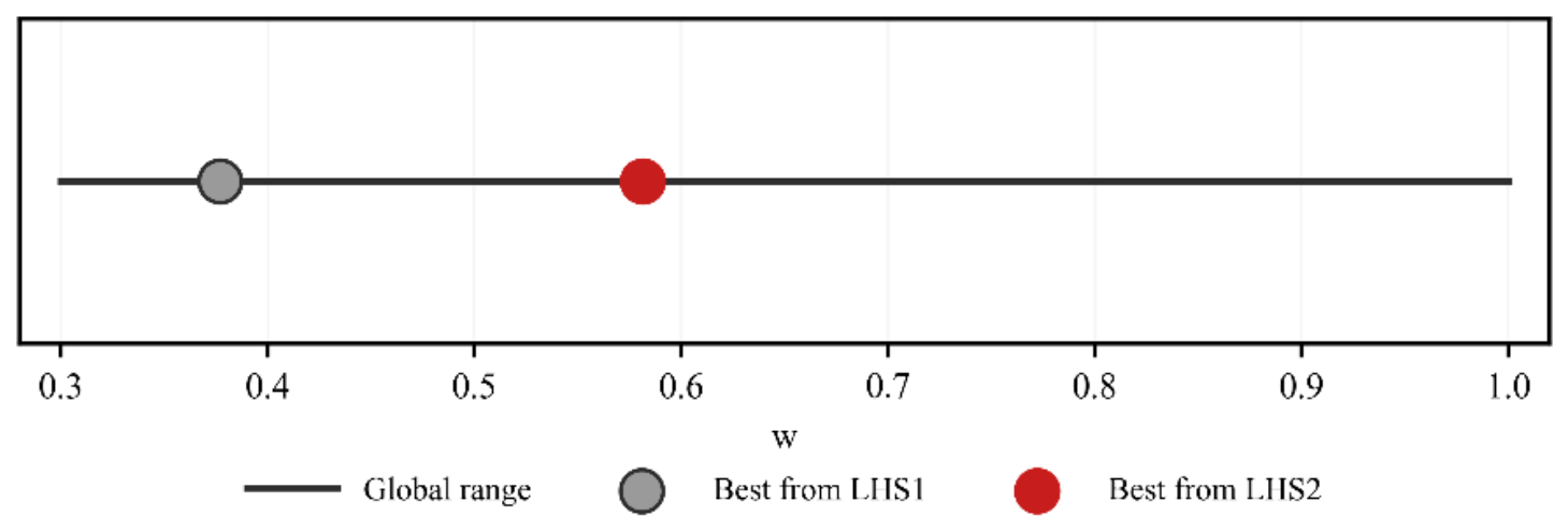
Furthermore, the evolution of parameter w during the optimization process is illustrated in Figure 11. The gray marker represents the best value obtained from the first stage, while the red marker corresponds to the optimal value obtained after the second-stage refinement. The shift in the optimal position demonstrates that the local search further improves the parameter combination.

Overall, the proposed two-stage LHS strategy enables efficient exploration of the multidimensional parameter space while maintaining a reasonable computational cost. By combining global exploration with local refinement, the optimal region can be progressively identified, leading to improved parameter configurations for the graded dielectric structure.

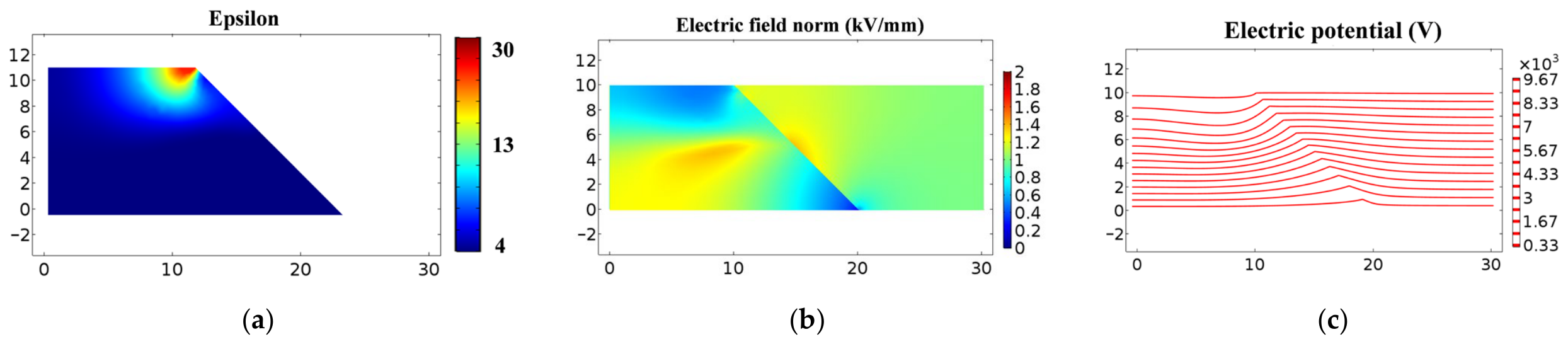
To further verify the effectiveness of the optimized parameter configuration, the electric field distribution corresponding to the optimal parameters obtained from the second-stage LHS search was analyzed. The final optimal parameters are p = 1.16147, q = 18.9053, w = 0.58145, ε_max = 26.127. The corresponding distributions of relative permittivity, electric field magnitude, and electric potential are illustrated in Figure 12. Figure 12a shows the distribution of relative permittivity in the optimized graded dielectric structure, where a high-permittivity region appears near the electrode. Figure 12b presents the electric field magnitude distribution, where the high-field region is reduced. Figure 12c shows the equipotential contours, which appear relatively smooth.

In summary, the two-stage Latin hypercube sampling approach enables efficient exploration of the design space and provides improved parameter configurations for the graded dielectric structure. However, LHS is essentially a sampling-based method, and its optimization efficiency may still be limited by the number of samples in large parameter spaces. In addition, it lacks a directed search mechanism toward the global optimum. Therefore, a more efficient optimization strategy is desirable. An improved optimization method will be introduced in the next section.

4. Response Surface Based Optimization

4.1. Overall Optimization Strategy

In Section 3, Latin hypercube sampling (LHS) was employed to explore the global parameter space and identify potential promising regions for the design variables. Although LHS provides good coverage of the parameter space, the sampling points are randomly distributed, making it difficult to establish a continuous functional relationship between the design variables and the objective function. As a result, the optimal parameter combination cannot be accurately determined using LHS alone.

To further improve the accuracy of parameter optimization, response surface methodology (RSM) is introduced based on the promising regions identified by LHS. By constructing surrogate models between design variables and the objective function, RSM can capture the variation trend of system responses with limited simulation cost and perform efficient parameter optimization on the response surface. To balance global exploration capability and local optimization accuracy, a three-stage response surface optimization strategy is adopted, including global screening, local refinement, and boundary verification. By progressively narrowing the design space, the optimization process evolves from global exploration to local optimization and final convergence verification.

4.2. Stage-1 Global Response Surface Analysis

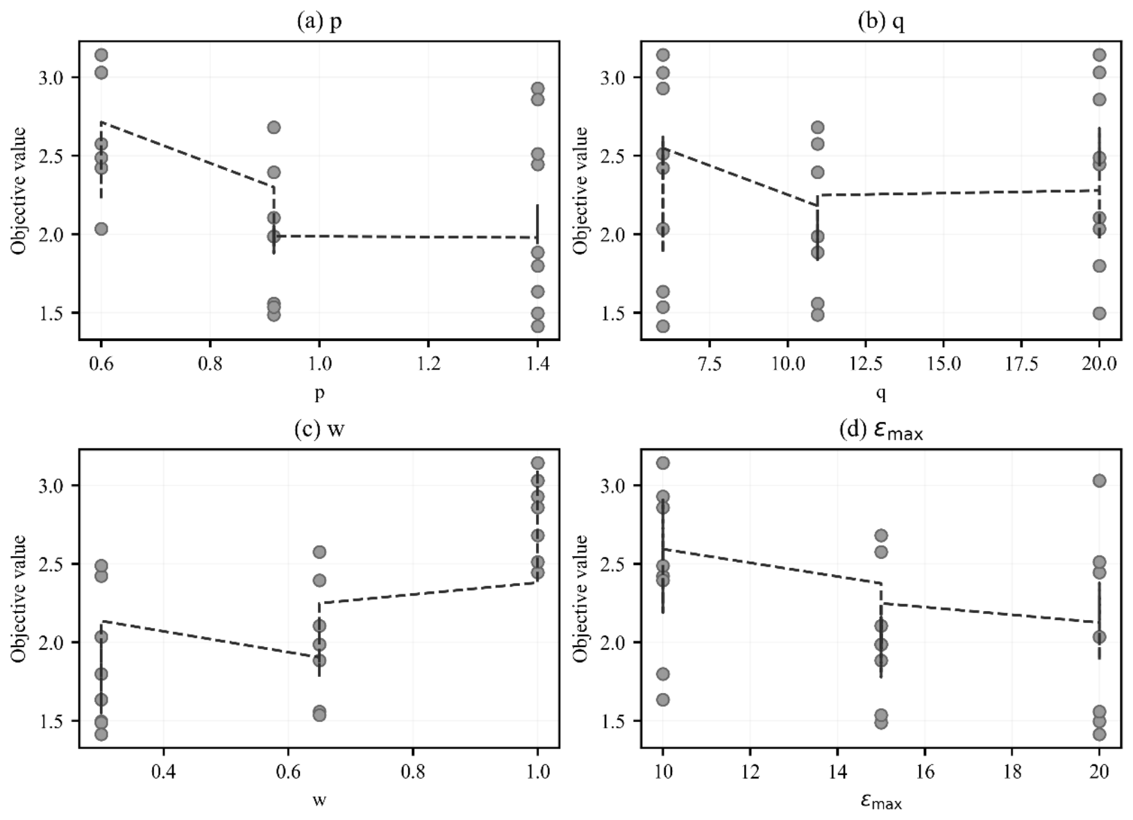
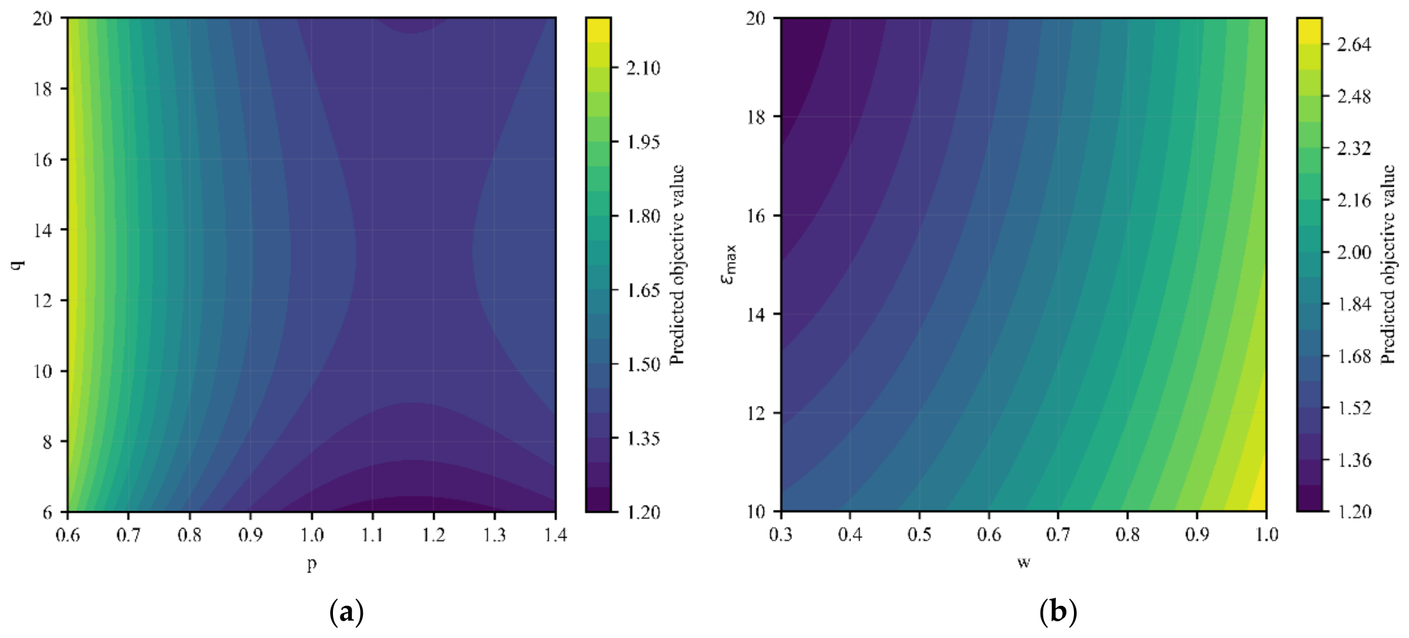
In the first stage, a four-factor face-centered central composite design (CCD) is employed within a relatively large design space, resulting in 29 simulation runs. Based on the simulation results, a second-order response surface model is constructed to analyze the influence of each design variable.

Figure 13 shows the main effects of the design variables on the objective function. It can be observed that the influences of the parameters are significantly different. In particular, p and w exhibit the most significant impact, whereas q and ε_max have relatively weaker effects.

Figure 14 further illustrates the response surfaces of typical parameter combinations. The response surfaces reveal a clear low-value region within the design space, which provides guidance for narrowing the design space in the next optimization stage.

The fitting results indicate that the coefficient of determination of the Stage-1 response surface model is R² = 0.9545, suggesting that the model can effectively capture the global relationship between the design variables and the objective function.

4.3. Stage-2 Local Response Surface Refinement

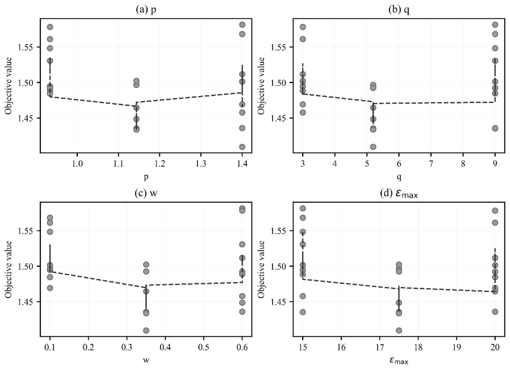
Based on the results obtained in Stage-1, the design space is reduced around the promising region and a new four-factor CCD experiment is constructed in Stage-2 to increase the sampling density near the optimal region and improve the fitting accuracy of the response surface model. A total of 31 simulation runs are performed in this stage. The main effects obtained in Stage-2 are shown in Figure 15. After the design space is reduced, the influence trends of the parameters become clearer.

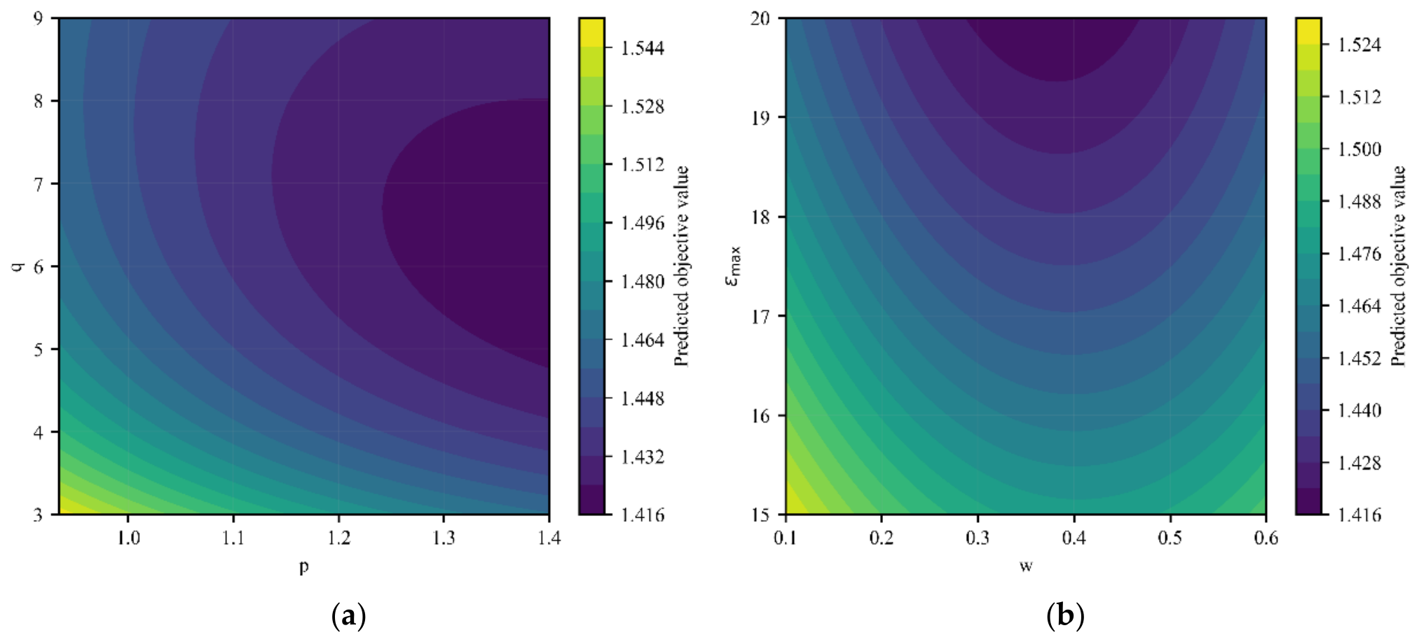
Among the parameters, w exhibits a noticeable local optimum, while p and ε_max remain close to their upper bounds. The response surface model predicts the optimal parameter combination as p = 1.4, q = 6.18355, w = 0.377724, ε_max = 20 with the corresponding objective value Obj = 1.40897.

The corresponding response surfaces are illustrated in Figure 16. The optimal region becomes more concentrated, indicating that the response surface model can accurately capture the local variation in the objective function.

4.4. Stage-3 Boundary Verification

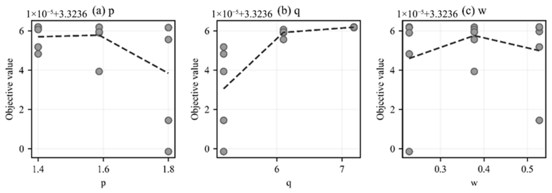
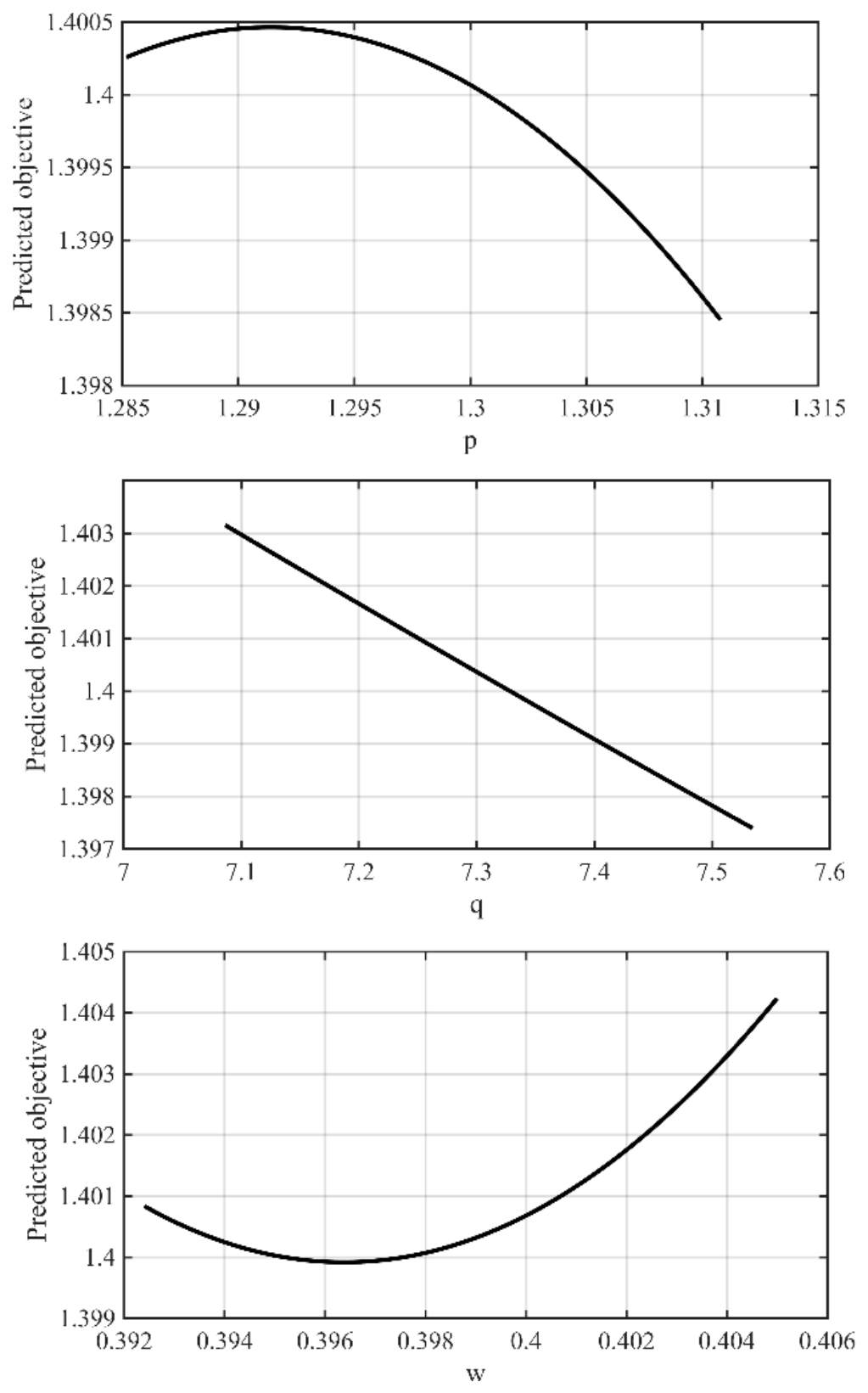
The results of Stage-2 indicate that the optimal solution lies near the parameter boundary. Therefore, in Stage-3 the parameter ε_max = 20 is fixed and a three-factor response surface model involving p, q, and w is constructed to further investigate the boundary region. A total of 21 simulation runs are performed in this stage. The main effects of the parameters are shown in Figure 17. The variation in the objective function becomes significantly smaller, indicating that the optimization process approaches convergence.

4.5. Model Validation and Residual Diagnostics

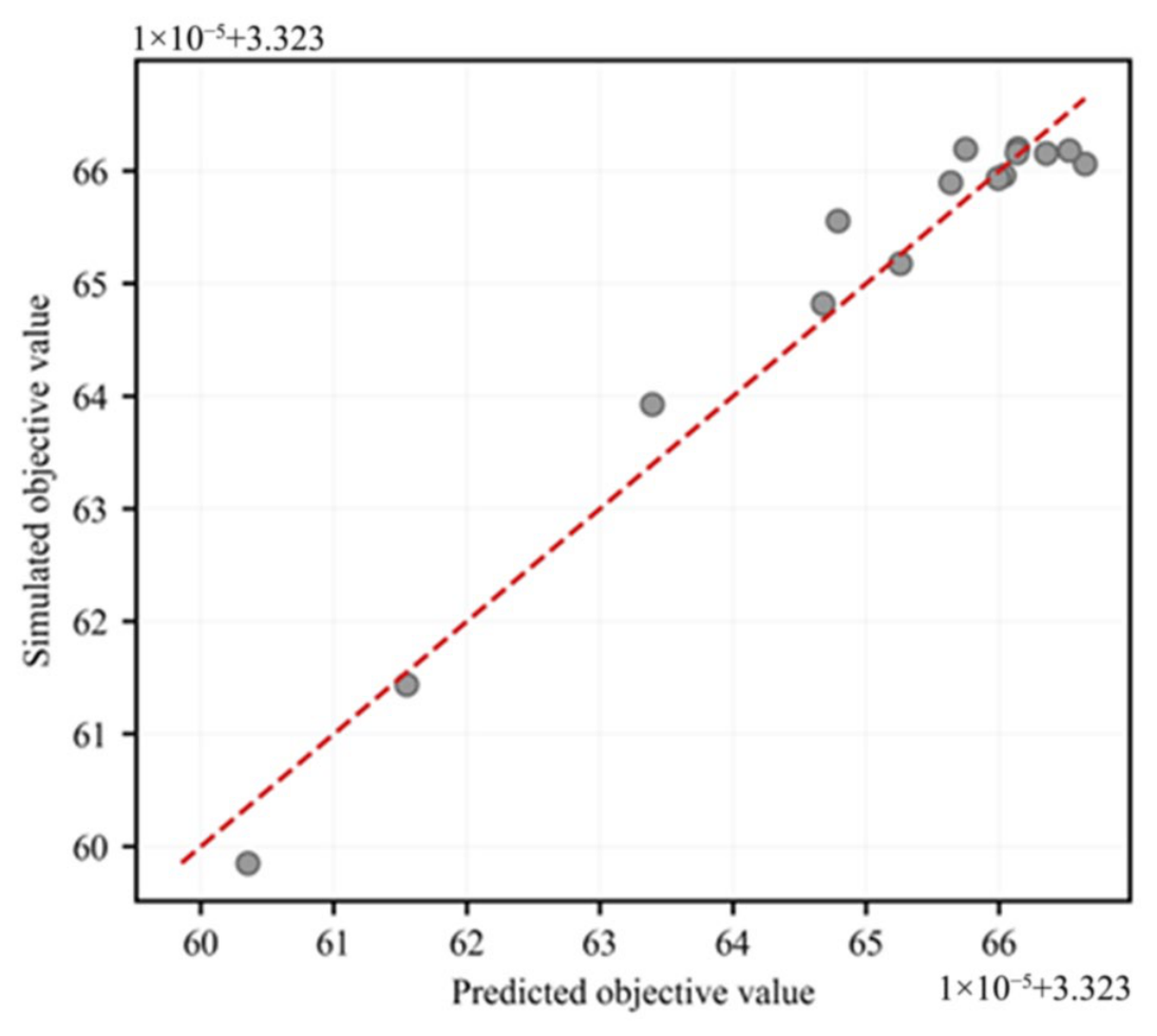
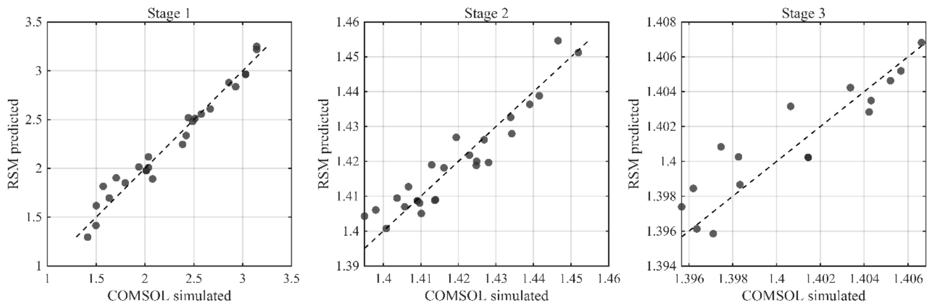
To evaluate the predictive capability of the response surface model, the predicted results are compared with the COMSOL simulation results. Figure 18 shows the comparison between predicted and simulated values. Most data points lie close to the diagonal line, indicating that the response surface model can accurately predict the variation in the objective function.

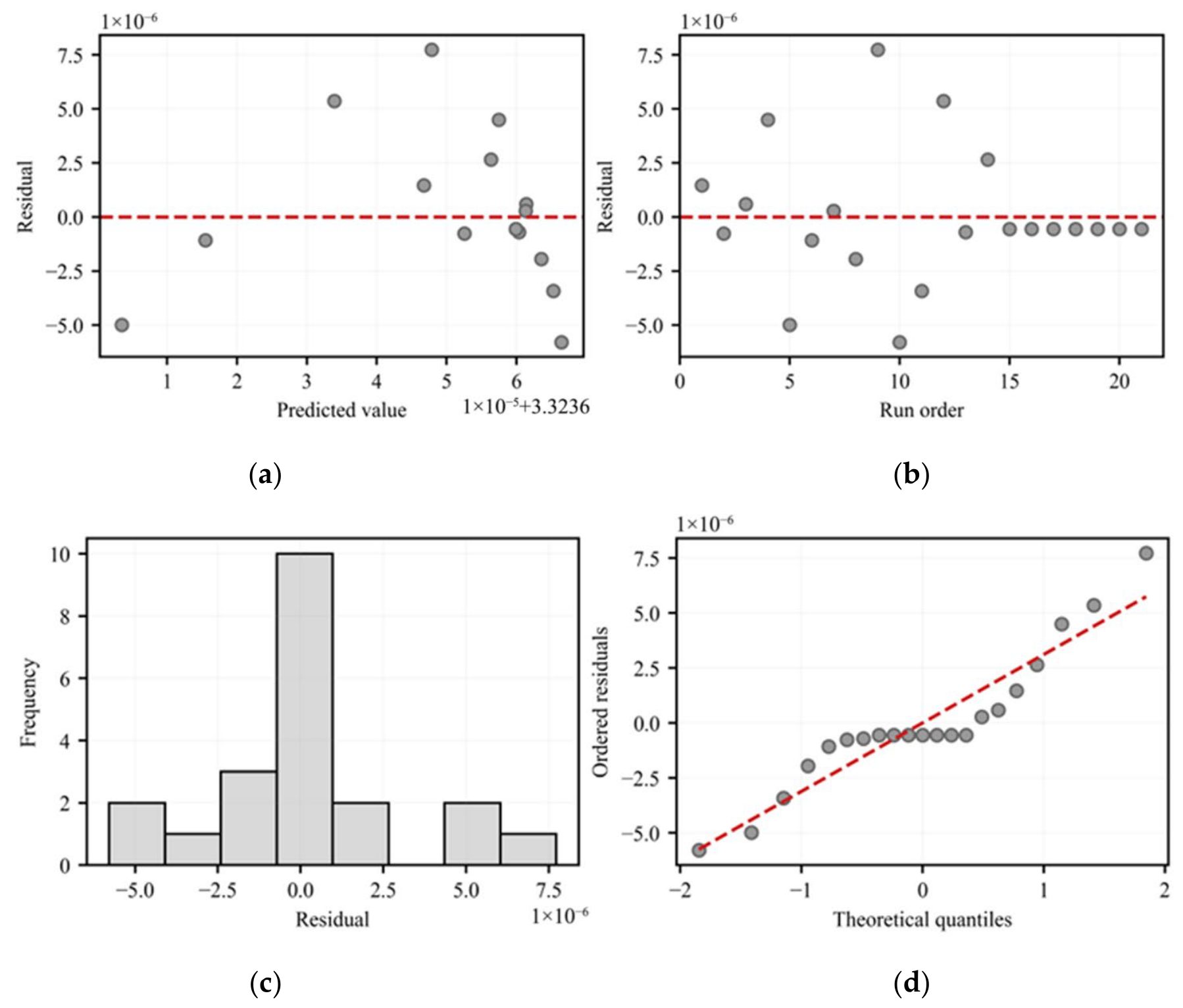
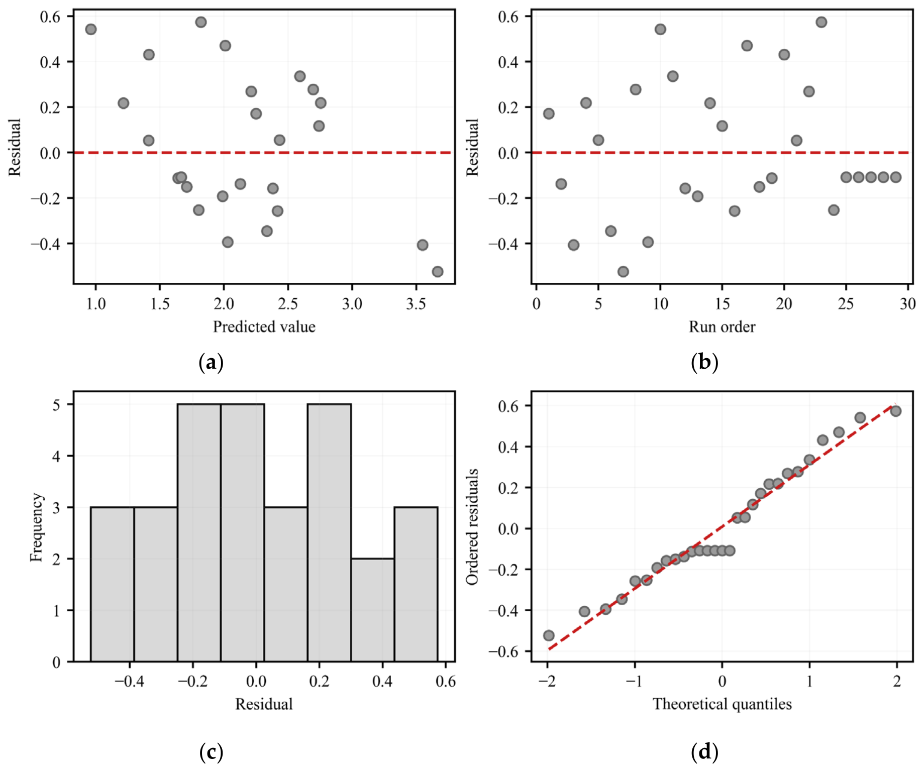
Figure 19 presents the residual diagnostic results, including residual versus predicted value, residual versus run order, residual histogram, and normal probability plot. The residuals are randomly distributed around zero without noticeable systematic bias, demonstrating that the response surface model has good statistical reliability.

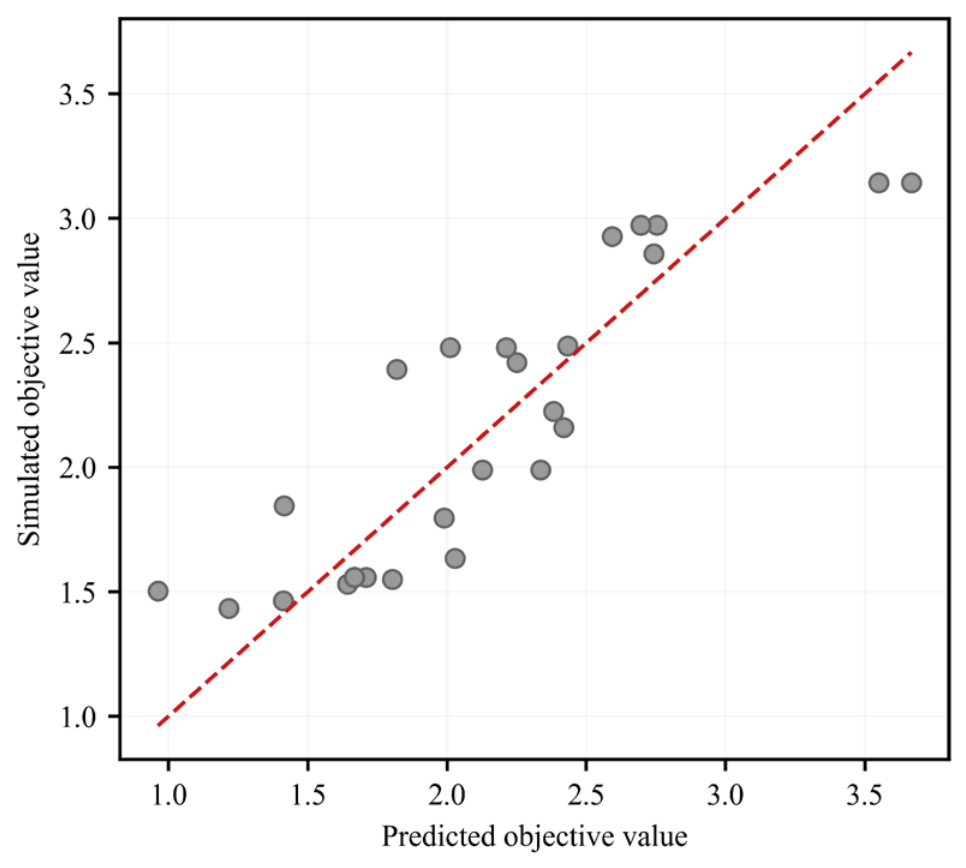
In addition to residual diagnostics, the potential risk of overfitting was further evaluated using leave-one-out cross-validation (LOOCV). In the LOOCV procedure, each sample was excluded in turn, and the response surface model was reconstructed using the remaining samples to predict the excluded point. The comparison between the LOOCV predicted values and the simulation results is shown in Figure 20, where most data points are still distributed close to the diagonal line, indicating acceptable prediction accuracy. The corresponding residual diagnostics based on LOOCV predictions are presented in Figure 21. The residuals remain randomly distributed around zero without significant systematic trends, further demonstrating the statistical reliability of the surrogate model.

The cross-validation results show that the prediction accuracy decreases compared with the training model, but the prediction error remains within an acceptable range. The cross-validated coefficient of determination (CV R²) is 0.7439, and the mean absolute percentage error (MAPE) is approximately 12.05%. These results indicate that the response surface model maintains reasonable generalization capability and does not exhibit severe overfitting. Therefore, the surrogate model can be reliably used for parameter optimization in this study.

4.6. Optimization Results and Transition to Hybrid Optimization

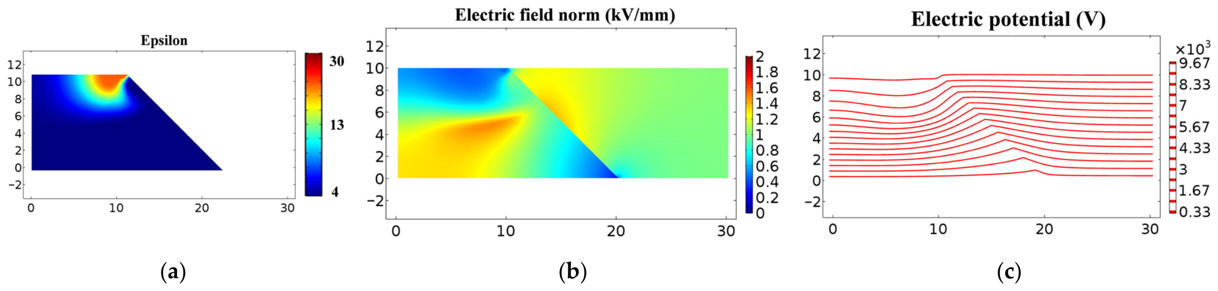
To further verify the physical validity of the optimized design, the dielectric permittivity distribution, electric field distribution, and electric potential distribution corresponding to the optimal parameters obtained in Stage-3 were recalculated using COMSOL, as shown in Figure 22.

As shown in Figure 22a, the optimized permittivity forms a gradient distribution near the high-field region, which effectively regulates the local electric field concentration. The corresponding electric field magnitude is presented in Figure 22b, where the high-field region is significantly alleviated and the overall electric field distribution becomes more uniform. Figure 22c illustrates the equipotential lines of the electric potential. The equipotential lines become smoother inside the structure, indicating that the potential gradient is effectively improved.

The three-stage response surface optimization gradually transitions from global exploration to local refinement and ultimately identifies a stable optimal parameter combination. However, the effectiveness of response surface optimization still depends on the selection of the initial design space. When the initial region deviates from the global optimum, the response surface model may still suffer from local optimal solutions.

Therefore, in the next section, the Latin hypercube sampling strategy introduced in Section 3 will be combined with the response surface optimization method presented in this section to develop a hybrid LHS–RSM optimization approach, aiming to further enhance the global search capability and robustness of the optimization process.

5. Optimization of Dielectric Gradient Parameters Based on the LHS–RSM Framework

5.1. Optimization Framework

In Section 3, Latin hypercube sampling (LHS) was employed to explore the global parameter space of the dielectric gradient design. The results showed that LHS is effective for identifying promising regions with relatively low objective values, but the sampling-based strategy alone is not sufficient to accurately determine the optimum because the relationship between the design variables and the objective function cannot be explicitly described. In Section 4, response surface methodology (RSM) was introduced to establish surrogate models for local parameter analysis and refinement. Although RSM provides efficient local optimization capability, its performance still depends on the selection of the initial design region.

To take advantage of both methods, a hybrid LHS–RSM optimization framework is developed in this section. In the proposed framework, LHS is first used to perform global exploration and select the top-performing candidate samples. These samples are then used to define a reduced parameter region for subsequent RSM optimization. Based on the reduced search space, a multi-stage response surface optimization procedure is carried out to progressively refine the parameter bounds and approach the final optimum. In this way, the global exploration capability of LHS and the local refinement capability of RSM are effectively combined.

5.2. LHS and Candidate Selection

In order to explore the global parameter space, Latin hypercube sampling was employed to generate candidate parameter combinations. Compared with conventional random sampling, LHS ensures a more uniform distribution of samples within the multidimensional design space. Each parameter range was divided into equal intervals, and the samples were generated to guarantee that each interval was represented exactly once.

For each sampled parameter combination, the objective value was evaluated using the response surface model established in Section 4. Among all generated samples, the top-performing candidates with the lowest objective values were selected as promising solutions.

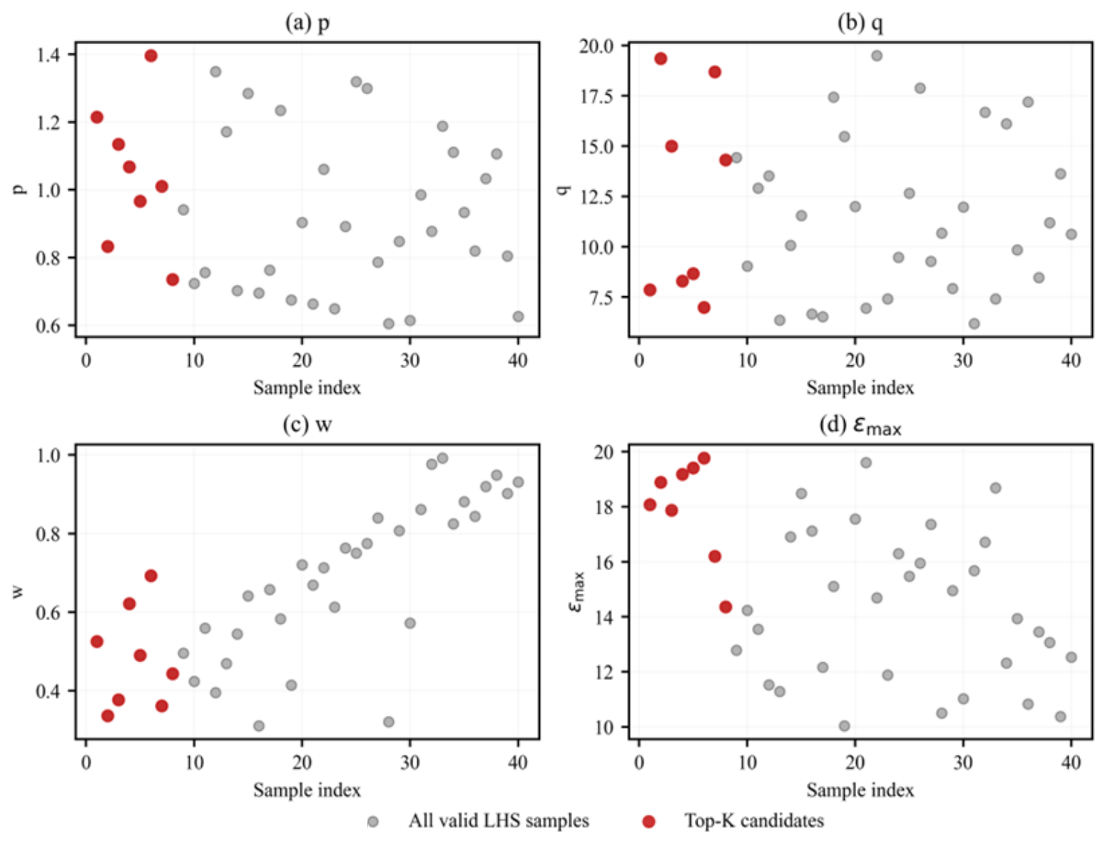
Figure 23 illustrates the distribution of LHS samples and the corresponding top-K candidates. It can be observed that the selected candidates are mainly concentrated within specific regions of the parameter space, indicating that these regions are more likely to contain the optimal solution.

5.3. Parameter Space Reduction

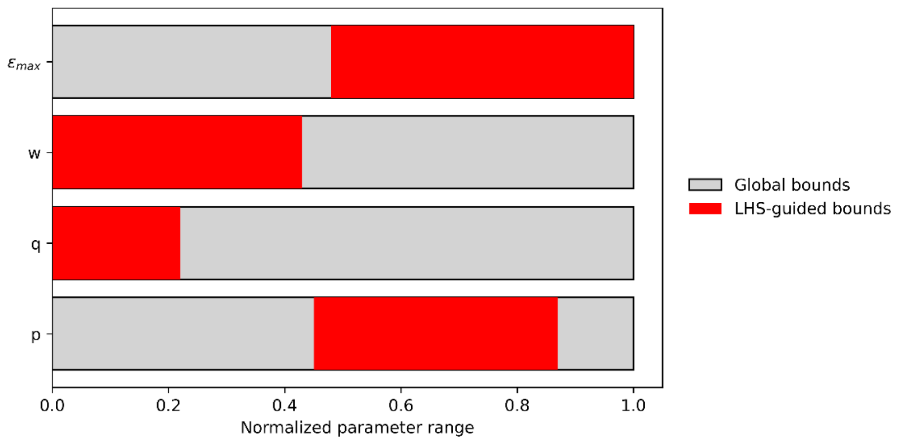
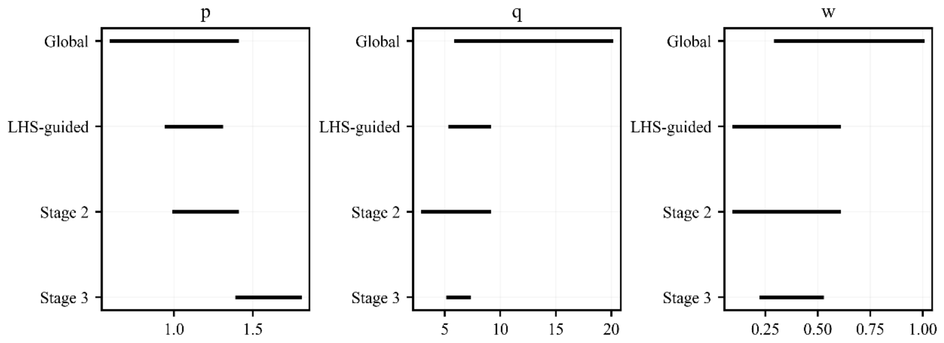
Based on the candidate solutions obtained from LHS, the parameter bounds were further refined to reduce the search space for subsequent optimization. Instead of exploring the entire global parameter space, the optimization process focuses on a reduced region surrounding the best-performing samples. Figure 24 presents the comparison between the global parameter bounds and the LHS-guided reduced bounds. It can be observed that the search space is significantly narrowed while still covering the most promising regions identified during the LHS exploration stage. The reduction in the parameter space not only improves optimization efficiency but also enhances the stability of the subsequent response surface optimization.

5.4. Progressive RSM Optimization

After determining the reduced parameter bounds, a multi-stage RSM optimization procedure was conducted to progressively approach the optimal solution. In each stage, the response surface model was used to evaluate the objective function and identify the optimal parameter combination within the current parameter bounds. Figure 25 illustrates the progressive refinement of the parameter bounds during the optimization process. As the optimization proceeds, the search space becomes increasingly concentrated around the optimal region.

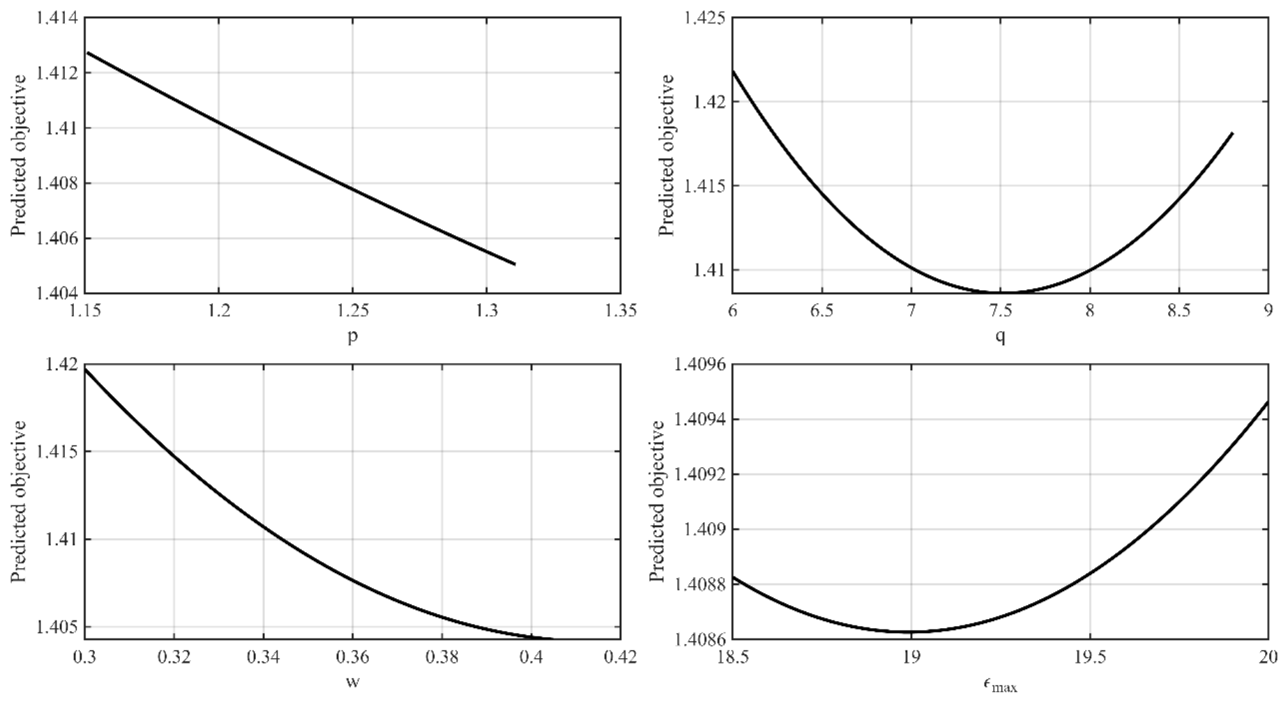
To further analyze the influence of each design variable, the main effects of the parameters were examined. Figure 26 and Figure 27 present the response curves of the objective function with respect to each parameter in different optimization stages. The results reveal the sensitivity of the objective function to the design variables and provide guidance for identifying the optimal parameter region.

5.5. Model Validation

To verify the reliability of the response surface model during the optimization process, several parameter combinations predicted by the RSM were validated using COMSOL simulations. The predicted objective values were compared with the corresponding simulated results. Figure 28 shows the comparison between the predicted and simulated objective values for different optimization stages. The data points are closely distributed around the diagonal line, indicating good agreement between the RSM predictions and the finite-element simulation results. This validation confirms that the response surface model maintains sufficient accuracy during the optimization process and can be reliably used to guide parameter optimization.

5.6. Comparison of Optimization Methods

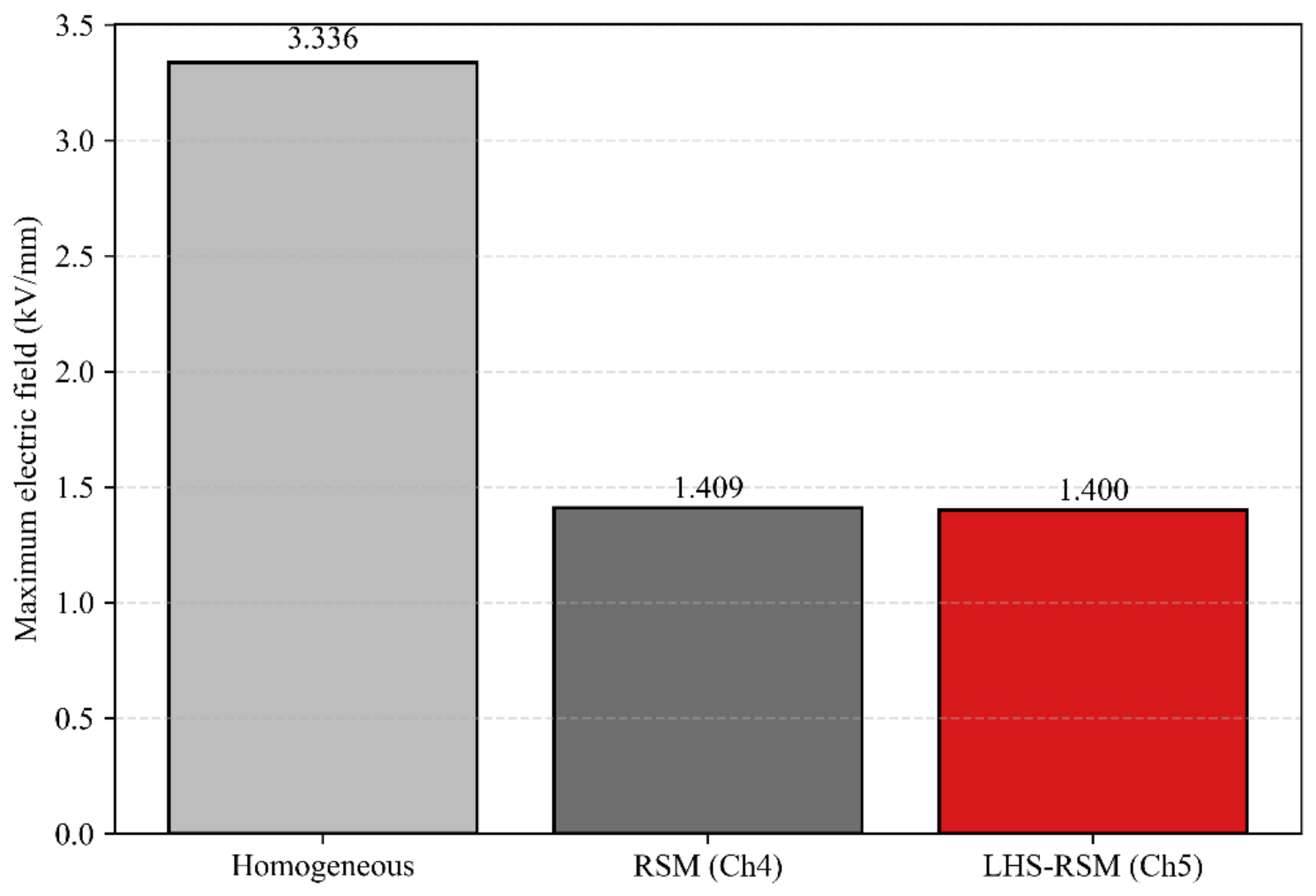
To further evaluate the effectiveness of the proposed optimization framework, the maximum electric field values obtained for different insulation configurations are compared. Figure 29 presents the maximum electric field for the homogeneous insulator, the optimized design obtained using response surface methodology (RSM) in Section 4, and the final design obtained using the proposed LHS–RSM optimization framework.

By further introducing the LHS–RSM optimization framework, the maximum electric field is reduced to 1.400 kV/mm. Although the reduction compared with the Section 4 result is relatively small, it demonstrates that the hybrid optimization strategy is capable of refining the dielectric gradient parameters and further improving the electric field uniformity. Compared with using RSM alone, the proposed LHS–RSM framework combines the global exploration capability of LHS with the local refinement capability of RSM. LHS is first employed to explore the global parameter space and identify promising regions, while RSM is then used to construct a response surface model for efficient local optimization. This hybrid strategy improves the robustness of the optimization process and avoids the risk of directly applying RSM in an excessively large design space.

Therefore, the LHS–RSM framework provides a more reliable and efficient approach for optimizing dielectric gradient insulation structures. Furthermore, cross-validation analysis also demonstrates that the surrogate model maintains acceptable prediction accuracy for unseen parameter combinations, indicating that the model has good generalization capability during the optimization process.

5.7. Optimization Performance Demonstration

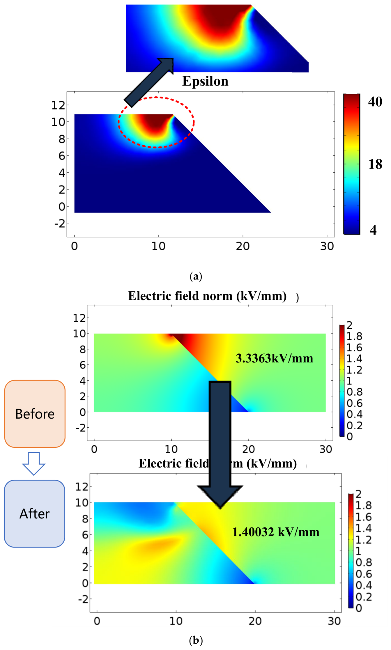
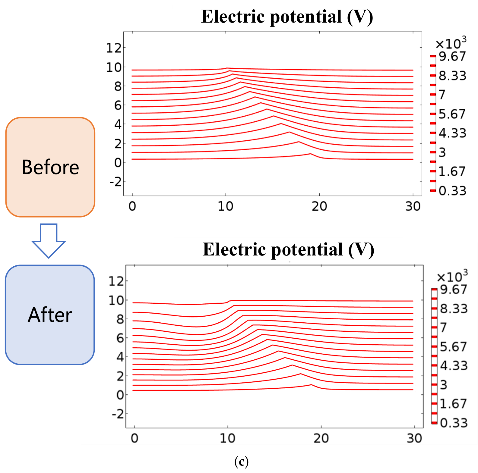
To verify the effectiveness of the optimized dielectric gradient parameters, the electric field and electric potential distributions before and after optimization are compared, using p = 1.310776, q = 7.534328, w = 0.396775, ε_max = 20, as shown in Figure 30.

5.8. Comparison with Conventional Optimization Methods

To quantitatively demonstrate the computational cost reduction and performance improvement of the proposed LHS–RSM framework, a comparison with the standard topology optimization method using conventionally determined parameters (e.g., empirical trial-and-error parameter selection as commonly used in traditional studies such as Li et al. [8]) was conducted.

In traditional parameter selection for topology optimization, the optimal combination of parameters is usually determined through repeated simulations or grid search in a high-dimensional parameter space. For example, a standard 5-level grid search in a four-parameter space would require 5⁴ = 625 independent topology optimization runs. Since each topology optimization run involves multiple finite element iterations, the overall computational cost is extremely high.

In contrast, the proposed LHS–RSM framework explores the parameter space using Latin Hypercube Sampling and constructs a response surface model to approximate the relationship between model parameters and optimization objectives. In this study, only 95 topology optimization evaluations were required to construct the surrogate model and perform parameter optimization, which significantly reduces the number of required simulations compared with traditional exhaustive parameter search methods.

In addition to computational efficiency, the proposed method also improves optimization performance. Using empirically selected parameters similar to those reported in the literature, the optimized maximum electric field (E_max) of the GIS insulator model is approximately 1.52 kV/mm. By contrast, the proposed LHS–RSM framework identifies a better parameter combination through systematic parameter space exploration and reduces E_max to 1.400 kV/mm. This comparison indicates that the proposed method not only reduces computational cost but also achieves improved electric field optimization performance.

6. Conclusions

This study proposes an efficient parameter optimization framework for dielectric gradient topology design of GIS insulators by integrating Latin Hypercube Sampling (LHS) and Response Surface Methodology (RSM). The main conclusions are summarized as follows.

(1)

A two-stage LHS strategy combined with multi-stage response surface optimization is developed to efficiently explore the multidimensional parameter space. The approach enables effective global exploration and local refinement, and the constructed response surface model achieves a high coefficient of determination (R² = 0.9545), indicating that the relationship between design variables and the objective function can be accurately captured.

(2)

By integrating the global exploration capability of LHS with the local optimization capability of RSM, the proposed hybrid LHS–RSM framework significantly improves optimization efficiency and robustness. The total number of simulations required is reduced to 161, whereas conventional single-parameter scanning with four parameters (20 levels each) would require approximately 160,000 simulations, representing a reduction of about three orders of magnitude in computational cost.

(3)

The optimized dielectric gradient parameters effectively improve the electric field distribution of the GIS insulator. Compared with the homogeneous insulation structure, the maximum electric field is reduced from 3.336 kV/mm to 1.400 kV/mm, demonstrating the effectiveness of the proposed framework in enhancing electric field uniformity and insulation performance.

Overall, the proposed LHS–RSM optimization framework provides a practical and efficient method for parameter selection in dielectric gradient topology design and has potential applications in other topology optimization problems involving complex multiparameter coupling.

Finally, while this study establishes a comprehensive theoretical and computational framework for parameter optimization, the physical realization of such dielectric gradient insulators is highly feasible using existing manufacturing technologies. Specifically, the optimized continuous gradient profile can be effectively approximated and fabricated through a step-by-step layered casting technique [21]. By discretizing the continuous permittivity distribution into several distinct macroscopic layers, epoxy resin composites with varying high-k filler concentrations can be sequentially cast and cured. Future experimental work will focus on manufacturing these layered gradient prototypes using this multi-step casting process to validate their insulation performance and electric field homogenization under actual high-voltage operational conditions.

References

1. Kindersberger, J.; Lederle, C. Surface Charge Accumulation on Insulators in DC Ion Flow Fields. IEEE Trans. Dielectr. Electr. Insul. 2008, 15, 941–948. [Google Scholar] [CrossRef] [Scilit]
2. Sun, G.; Zhao, Y.; Liu, J.; Zhang, X.; Wang, J.; Wang, J.; He, Z.; Gao, Y.; Zhang, X.; Wang, D. Secondary Electron Emission and Trap State In Situ Combined (SETiC) Measurement for Spacecraft ESD Protection. IEEE Trans. Instrum. Meas. 2026, 75, 1–10. [Google Scholar] [CrossRef] [Scilit]
3. Donzel, A.; Schuler, M.; Stevens, G.C. Nonlinear Electrical Conduction in Polymer Composites for Field Grading in High-Voltage Applications: A Review. Polymers 2021, 13, 1370. [Google Scholar] [CrossRef] [Scilit]
4. Okubo, H.; Shumiya, H.; Ito, M.; Kato, K. Optimization Techniques on Permittivity Distribution in Permittivity Graded Solid Insulators. In Proceedings of the Conference Record of the 2006 IEEE International Symposium on Electrical Insulation; IEEE: Toronto, ON, Canada, 2006; pp. 519–522. [Google Scholar]
5. Kurimoto, M.; Kato, K.; Shikari, Y.; Hoshina, Y.; Takei, M.; Okubo, H. Application of functionally graded material for reducing electric field on electrode and spacer interface. IEEE Trans. Dielectr. Electr. Insul. 2010, 17, 256–263. [Google Scholar] [CrossRef] [Scilit]
6. Seok, J.M.; Choi, H.S.; Baek, M.K.; Park, I.H. Optimization of Permittivity Distribution for Functionally Graded Material in GIS Spacer. IEEE Trans. Magn. 2012, 48, 747–750. [Google Scholar] [CrossRef]
7. Lee, K.H.; Hong, S.G.; Baek, M.K.; Choi, H.S.; Kim, Y.S.; Park, I.H. Alleviation of Electric Field Intensity in High-Voltage System by Topology Shape Optimization of Dielectric Material Using Continuum Design Sensitivity and Level Set Method. IEEE Trans. Magn. 2015, 51, 7001404. [Google Scholar] [CrossRef] [Scilit]
8. Li, W.; Li, X.; Guo, B.; Wang, C.; Liu, Z.; Zhang, G. Topology Optimization of Truncated Cone Insulator with Graded Permittivity Using Variable Density Method. IEEE Trans. Dielectr. Electr. Insul. 2019, 26, 1–9. [Google Scholar] [CrossRef] [Scilit]
9. Guo, D.; Zhang, G.; Liu, J.; Wang, C.; Zhang, X. The Influence of Gas Conductivity on the Surface Charge Accumulation Characteristics of DC-GIS/GIL Insulators. IEEE Trans. Dielectr. Electr. Insul. 2026; early access.
10. Vasconcelos, J.A.; Krahenbuhl, L.; Nicolas, A. Optimization of a high-voltage insulator profile using a genetic algorithm. IEEE Trans. Magn. 1997, 33, 1856–1859. [Google Scholar] [CrossRef] [Scilit]
11. Goldberg, D.E. Genetic Algorithms in Search, Optimization and Machine Learning; Addison-Wesley: Reading, MA, USA, 1989. [Google Scholar]
12. Kennedy, J.; Eberhart, R. Particle Swarm Optimization. In Proceedings of ICNN′95—International Conference on Neural Networks; IEEE: Perth, Australia, 1995; pp. 1942–1948. [Google Scholar]
13. Ilkhechi, H.D.; Samimi, M.H. Applications of the Machine Learning in High-Voltage Engineering: A Review. IEEE Trans. Dielectr. Electr. Insul. 2021, 28, 438–454. [Google Scholar] [CrossRef] [Scilit]
14. Sun, Y.; Li, J.; Chen, M.; Zhu, W.; Yao, H.; Du, B. Multi-objective Structure Design of ±550 kV DC Gas Insulated Cable Termination via a Two-Layer Stacking Optimization Surrogate Model. IEEE Trans. Dielectr. Electr. Insul. 2025; early access.
15. Junior, K.U.; Lucchini, F.; Marconato, N. Data-Driven Dynamics Learning on Time Simulation of SF6 HVDC-GIS Conical Solid Insulators. Electronics 2025, 14, 616. [Google Scholar] [CrossRef] [Scilit]
16. Kim, H.K.; Hwang, Y.S.; Park, I.H. Optimization of high voltage insulator profile using response surface methodology. IEEE Trans. Magn. 2007, 43, 1593–1596. [Google Scholar]
17. Sima, W.; Sun, P.; Yang, M. Optimization of grading ring parameters for ±800 kV converter valve based on 3-D electric field and orthogonal experimental design. IEEE Trans. Dielectr. Electr. Insul. 2012, 19, 168–176. [Google Scholar]
18. McKay, M.D.; Beckman, R.J.; Conover, W.J. A Comparison of Three Methods for Selecting Values of Input Variables in the Analysis of Output from a Computer Code. Technometrics 1979, 21, 239–245. [Google Scholar] [CrossRef] [Scilit]
19. Myers, R.H.; Montgomery, D.C.; Anderson-Cook, C.M. Response Surface Methodology: Process and Product Optimization Using Designed Experiments; Wiley: Hoboken, NJ, USA, 2016. [Google Scholar]
20. Sun, G.; Zhao, Y.; Gao, Y.; Wang, J.; Wang, J.; Zhang, X.; Wang, D.; He, Z.; Zhang, X.; Liu, J. Ultra-High-Efficiency On-Chip CO2 Conversion by Nanosecond Self-Pulsing Micro-Plasma Devices. Carbon Energy 2026, 8, e70010. [Google Scholar] [CrossRef] [Scilit]
21. Qasim, S.A.; Gupta, N. Computation of effective properties of graded and layered dielectrics. IEEE Trans. Dielectr. Electr. Insul. 2021, 28, 460–467. [Google Scholar] [CrossRef] [Scilit]
Figure 1. Geometry of the 45° truncated cone insulator [8].
Electronics 15 03698 g001
Figure 2. Electric field distribution of the conical GIS insulator obtained.
Electronics 15 03698 g002
Figure 3. Mesh independence verification for the electrostatic simulations. (a) Variation in the maximum electric field (Emax) with different minimum mesh sizes. (b) Relative change in Emax during mesh refinement, the red dashed line indicates the 1% convergence criterion.
Electronics 15 03698 g003
Figure 4. Overall workflow of the proposed LHS–RSM hybrid optimization framework, illustrating the systematic transition from the initial configuration to the optimized model through global parameter exploration, sub-region determination, and surrogate modeling.
Electronics 15 03698 g004
Figure 5. Sampling distributions of the design variables in the first-stage Latin hypercube sampling (LHS). Each parameter is uniformly distributed within its predefined global range.
Electronics 15 03698 g005
Figure 6. Relationships between the design variables and the objective value obtained from the first-stage LHS. Gray points denote sampled solutions, the dashed curve indicates the trend of the data, and the red marker represents the best solution.
Electronics 15 03698 g006
Figure 7. Normalized positions of the optimal parameters obtained from the first-stage LHS within the global design ranges. The dashed lines indicate the normalized parameter intervals, and the red markers denote the optimal parameter values.
Electronics 15 03698 g007
Figure 8. Relationships between the design variables and the objective value obtained from the second-stage LHS within the refined parameter space. Gray dots denote sampled solutions, the dashed curve indicates the trend of the data, and the red markers represent the best solution.
Electronics 15 03698 g008
Figure 9. Normalized positions of the optimal parameters obtained from the second-stage LHS within the global parameter ranges. The red markers indicate the optimal parameter values, while the dashed lines represent their projected normalized positions within the design interval.
Electronics 15 03698 g009
Figure 10. Comparison between the results obtained from the first-stage and second-stage LHS optimization. (a) Distribution of objective values. (b) Comparison of normalized optimal parameters, where the dotted lines indicate the normalized boundary limits of the design interval.
Electronics 15 03698 g010
Figure 11. Evolution of the optimal value of parameter w during the two-stage optimization process. The gray marker represents the best solution from the first stage, while the red marker corresponds to the refined solution from the second stage.
Electronics 15 03698 g011
Figure 12. Electric field characteristics of the optimized graded dielectric structure obtained from the two-stage LHS optimization. (a) Relative permittivity distribution. (b) Electric field magnitude distribution. (c) Electric potential contours.
Electronics 15 03698 g012
Figure 13. Main effects of design variables on the objective function in Stage-1 response surface analysis. The gray dots denote sampled data, and the dotted lines represent the fitted main-effect trends.
Electronics 15 03698 g013
Figure 14. Response surface distributions of the objective function for representative parameter combinations in Stage-1: (a) p q interaction, (b) w ε m a x interaction.
Electronics 15 03698 g014
Figure 15. Main effects of design variables on the objective function in Stage-2 local response surface refinement. The gray dots denote sampled data, and the dotted lines represent the fitted main-effect trends.
Electronics 15 03698 g015
Figure 16. Response surface distributions near the optimal region obtained in Stage-2: (a) p q response surface, (b) w ε m a x response surface.
Electronics 15 03698 g016
Figure 17. Main effects of design variables in Stage-3 boundary verification: (a) p, (b) q, and (c) w. The gray dots denote sampled data, and the dotted lines represent the fitted main-effect trends. Further analysis shows that the variation in the objective function is only on the order of 10−5, indicating that the system has reached a stable optimal state.
Electronics 15 03698 g017
Figure 18. Comparison between predicted objective values obtained from the response surface model and COMSOL simulation results. The gray dots denote sampled data, and the red dashed line represents the ideal parity line (y = x).
Electronics 15 03698 g018
Figure 19. Residual diagnostics of the response surface model: (a) residuals versus predicted values, (b) residuals versus run order, (c) residual histogram, and (d) normal probability plot. The red dashed lines indicate the reference baselines used for residual evaluation and normality assessment.
Electronics 15 03698 g019
Figure 20. Parity plot between LOOCV predicted objective values and COMSOL simulated results.
Electronics 15 03698 g020
Figure 21. Residual diagnostics based on LOOCV predictions: (a) residuals versus predicted values, (b) residuals versus run order, (c) residual histogram, and (d) normal probability plot. The red dashed lines represent the zero-reference baselines in (a,b), and the fitted reference line for normality assessment in (d).
Electronics 15 03698 g021
Figure 22. Field distributions corresponding to the optimized parameters obtained from the RSM optimization. (a) Relative permittivity distribution. (b) Electric field magnitude distribution. (c) Electric potential distribution.
Electronics 15 03698 g022
Figure 23. Distribution of top candidate solutions obtained from LHS.
Electronics 15 03698 g023
Figure 24. Comparison between the global parameter bounds and the LHS-guided reduced bounds.
Electronics 15 03698 g024
Figure 25. Progressive reduction in the design space during the LHS–RSM optimization process.
Electronics 15 03698 g025
Figure 26. Main effects of design parameters on the predicted objective value obtained from the response surface model (Stage 2).
Electronics 15 03698 g026
Figure 27. Main effects of design parameters on the predicted objective value obtained from the response surface model (Stage 3).
Electronics 15 03698 g027
Figure 28. Comparison between RSM predicted values and COMSOL simulated results at different optimization stages.
Electronics 15 03698 g028
Figure 29. Comparison of maximum electric field values for different insulation configurations.
Electronics 15 03698 g029
Figure 30. Optimization performance of the dielectric gradient insulator. (a) Relative permittivity distribution. (b) Electric field magnitude distribution. (c) Electric potential distribution. The arrow indicates the transition from the initial design (Before) to the optimized design (After).
Electronics 15 03698 g030aElectronics 15 03698 g030b