Efficient Membership Function Computation Using a Modified Bisection Algorithm

Abstract

Fuzzy set theory, proposed by Lotfi Zadeh, is applied with great success in embedded, control-oriented systems based on microcontrollers or programmable logic devices. Algorithms used in these systems operate on fuzzy sets represented by membership functions. In practically implemented control systems, these functions typically possess simple linear shapes, such as trapezoidal or triangular. To compute the function value, the classical method relies on multiplication and division. These operations are complex to implement in software or hardware, consume significant resources, and are time-consuming. This paper proposes a fixed-point computation method to obtain the value of a membership function without relying on these operations. For this purpose, the bisection algorithm was adopted, replacing its complex arithmetic with addition and binary shift operations. This approach allows for a reduction in computation time and the hardware or software overhead required by resource-constrained embedded systems, especially architectures without dedicated hardware accelerators for multiplication and division. Sample software and hardware implementations demonstrate its suitability for real-world systems.

1. Introduction

Practical implementations of fuzzy inference systems in embedded systems involve hardware solutions (based on programmable logic devices such as FPGAs, CPLDs, or ASIC chips) [1,2,3] or, more frequently, software solutions (embedded software for general-purpose microcontrollers) [4,5]. These systems implement fuzzy inference algorithms that perform calculations on fuzzy data represented by membership functions [6,7].

Regardless of the inference strategies and fuzzy operators used, calculations are performed on these functions using classical arithmetic operations [8,9]. The most basic operation is calculating the value of the membership function, which typically requires addition, multiplication, and division [10,11]. While addition is fundamental to binary arithmetic, the other operations are often replaced by binary shifts (equivalent to multiplication or division by a power of 2) and repeated additions [12,13]. However, replacing one complex operation with several basic ones can ultimately increase computation time or resource consumption. Therefore, alternative methods should be sought to significantly improve performance while reducing resource requirements [14].

From an application perspective, aspects related to membership functions can be considered in three interconnected areas: the typology of functions and their scope of application along with selection criteria, algorithmic methods for determining numerical values of the functions, and techniques for their formal representation in data structures.

Membership functions can be divided into two basic classes, depending on their mathematical properties and application domain: piecewise linear functions (e.g., triangular or trapezoidal), which are typically used in embedded systems and control systems (automation), and smooth functions differentiable at every point (e.g., Gaussian or bell-shaped), which play a crucial role in optimization and machine learning. The application area of these functions is often determined by computational complexity, which translates directly into hardware overhead and the execution time required to calculate the function values [15,16]. For this reason, where smooth functions are required, they are often formulated as spline curves within the specifications—i.e., low-degree polynomial functions (most commonly third-degree, so-called cubic splines) [17,18,19]—or, in the simplest case, they are approximated by piecewise linear functions [20,21], using, for instance, the method of membership function decomposition into alpha-cuts [22]. By appropriately selecting the number of partition points (knots), any arbitrary shape of the original function can be precisely replicated [23].

It is estimated, piecewise linear functions (triangular and trapezoidal) dominate in most practical implementations, accounting for over 70% of applications, which stems from their minimal resource requirements [24]. In turn, smooth nonlinear functions, such as the Gaussian function, represent approximately 15–20% of applications, while the less frequently used generalized bell function accounts for a mere 3–5% of systems. Meanwhile, sigmoidal functions, splines, and PI/S/Z-type polynomials constitute only about 2–3% of systems [25]. It is clearly evident that the continuous, piecewise linear function is the dominant and crucial function in fuzzy systems.

The type of membership function (membership in a specific class) is inherently linked to the method used to determine its value at a given point. There is a range of methods, which include classical methods (directly from the definition or mathematical formula) [26], the incremental method (also known as the finite difference method) [27], the method based on the CORDIC algorithm [28], and the utilization of specialized accelerators to calculate membership function values [29].

In the case of classical methods, the RAM requirement for storing function coefficients is low, and they can be modified on the fly, which is critical for adaptive systems. The precision of the calculated outcome depends on the adopted number representation system (integer, fixed-point, or real/floating-point type). Disadvantages include high and variable, yet predictable, computational overhead and execution time for determining the result, caused by the necessity of using multiplication, division, and the direct evaluation of non-linear functions, posing a challenge for resource-constrained hardware architectures [30].

The incremental method allows for saving computational power by replacing multiplication operations with addition, which directly translates into high performance [31]. The implementation is straightforward; the algorithm requires only a loop and a basic summation operation at each step (for more complex functions, more operations must be performed). Memory requirements are low, as the system stores only the current value and a constant increment. However, the accuracy of this method depends on the number of steps, which is not constant; thus, the time required to determine the result is variable. Operating on increments also leads to the accumulation of round-off errors. Furthermore, initializing the initial increment value or changing its step size during calculations requires the use of multiplication and division.

The CORDIC algorithm is widely used when the membership function is based on trigonometric, hyperbolic, exponential, or logarithmic functions (e.g., bell-shaped or sigmoidal functions) [32,33]. It computes advanced mathematical functions using a sequence of simple operations: bit shifts and additions, making it highly efficient for basic microcontrollers and FPGA devices. Avoiding complex operations during the function evaluation phase typically requires executing intricate operations at an earlier stage-variable initialization—which constitutes a data preprocessing bottleneck. These can be executed in linear mode (multiplication, division); however, for simple functions, the gain from the function evaluation itself may be overshadowed by the losses incurred during the preliminary stage. This is particularly significant for systems that require frequent adjustments of function parameters (tuning, adaptive systems).

Specialized accelerators rarely rely on a single technique; they generally combine the aforementioned evaluation methods with hardware-assisted computation (parallel and vector processing, pipelined architectures) and efficient data storage and processing methods (double buffering, multi-port memories) [34]. Despite the extreme performance of these circuits, they suffer from high implementation costs, structural rigidity (being tailored to strictly defined functions and fuzzy algorithms), and substantial system complexity. These characteristics significantly hinder their direct and fair comparison with simpler, single-chip solutions based on a single computational technique [29].

The representation of a membership function as a data structure is inherently linked to the memory architecture and its available capacity, as well as the computational overhead associated with evaluating its value. Usually, three description methods are employed: parametric, segmented, or tabular.

For the parametric description, the shape of the function is defined by a set of geometric points (e.g., four points for a trapezoid: $(a,b,c,d)$) or analytical parameters (e.g., the mean $\left(\mu \right)$ and standard deviation $\left(\sigma \right)$ for a Gaussian function). The function value is calculated directly from the formula or by applying the techniques described above.

The segmented form of a function is typically used for non-linear functions that are approximated by a sequence of segments or polynomials (splines). For each segment, the data structure stores a set of coefficients and the interval boundaries. Evaluating the function value reduces to determining the specific interval containing the target point (introducing additional computational overhead), where the value is then calculated in the same manner as in the parametric description.

In the tabular approach, the function is sampled and stored in ROM/RAM as a discrete vector of values (a LUT array, where values are precalculated using parametric or segmented methods). This enables instantaneous value retrieval (eliminating computation) and offers universality for any arbitrary function shape. However, memory consumption increases exponentially with bit resolution and the number of samples; therefore, data compression techniques are often additionally applied, such as removing repeating values in the simplest case or employing differential encoding. Nonetheless, reading the value involves on-the-fly data decompression and requires extra hardware logic or processor instructions. If the function coefficients need to be modified, the entire array must be recomputed, which often requires implementing an computation module that remains active only during array initialization [35].

In conclusion, a comparison of the fundamental properties of the discussed methods is summarized in

Table 1. Comparison of membership function computation methods parameters.

Method	Computation Time	Memory Requirements	Accuracy	Implementation Complexity
LUT (Compression)	Lowest	Very high	Depends on table size	Very low
Piecewise-Linear Approximations	Medium–high	Low	Depends on mbf (error for curves)	Medium
Incremental Computations	Low	Minimal	High	Medium
CORDIC-based Methods	Medium	Very low	Very high	Medium/High
Specialized Hardware Accelerators	Very low	Hard blocks (e.g., BRAM, DSP)	Maximum	Very high

.

Taking the above into consideration, parametric linear membership functions can be identified as the most universal and frequently used in practice, and they can be easily extended to segmented functions (piecewise linear approximation). Regarding the methods for evaluating function values, the execution of the algorithms is two-stage and comprises: initialization, performed only once, and the actual computation, executed in a loop.

In most cases, the cited methods eliminate complex multiplication and division operations from the evaluation phase, but conversely, they utilize them during the initialization stage. The proposed computation method fills this gap and offers the elimination of these operations at both the initialization and evaluation stages. Furthermore, the absence of multiplication and division allows for its implementation on any software and hardware platforms, regardless of whether they provide hardware support for complex mathematical operations. To maintain full generality of the ongoing considerations, the classical method for evaluating membership function values will be adopted as the reference point. This approach will allow for an objective evaluation of the efficiency of the proposed solution.

The paper is organized as follows: in Section 2 theoretical background of fuzzy algorithms, membership function representation, and classical methods of calculating membership values. The proposed bisection algorithm is described in Section 3, while its implementation, experimental results and discussion are presented in Section 4. Finally, Section 5 concludes the work.

2. Theoretical Backgrounds

Fuzzy inference result for a K-input MISO system is computed based on current inputs ${\mathit{x}}^{\prime }=[x_1^{\prime },x_2^{\prime },\dots ,x_K^{\prime }]$ and information in the knowledge base $KB[X_1,\dots ,X_K,Y]$ of the fuzzy system [6]. The knowledge base has the primary form of rule base $RB=\{R_1,R_2,\dots ,R_R\}$ and definitions of the linguistic variables (denoted as $X_1,\dots ,X_K$ and Y for inputs and output, respectively)  [7].

$$\mathrm{IF}\left(X_{1}is{\underline{A}}_{1r}\right)\mathrm{AND}\dots \mathrm{AND}\left(X_{K}is{\underline{A}}_{Kr}\right)\mathrm{THEN}\left(Yis{\underline{B}}_r\right),$$

(1)

where $\mathit{X}=[X_1,\dots ,X_K$], Y are linguistic variables, while $\underline{\mathit{A}}=[{\underline{A}}_{1r},\dots ,{\underline{A}}_{Kr}]$, ${\underline{B}}_r$ are linguistic values defined for the corresponding variables and described by the membership functions ${\mu }_{A_{1r}}\left(x_1\right),\dots ,{\mu }_{A_{Kr}}\left(x_K\right),{\mu }_{B_r}\left(y\right)$ of fuzzy sets $A_{1r},\dots ,A_{Kr},B_r$ respectively [36,37]. Practically implemented fuzzy systems usually use triangular or trapezoidal shape of membership functions ${\mu }_{A_{1r}}\left(x_1\right),\dots ,{\mu }_{A_{Kr}}\left(x_K\right)$ and singleton membership functions ${\mu }_{B_r}\left(y\right)$ (zero-order Takagi-Sugeno model) to simplify computations and thus improve system performance [5,38].

The output of the system is computed, according to the fuzzy inference algorithm, in four steps [13,36,37,38,39]:

• Fuzzification—The membership functions defined on the input variables $\mathit{X}$ are applied to their actual values ${\mathit{X}}^{\mathsf{\prime }}$ to determine the degree of truth for each rule premise (the if-parts of the rules (1)). The most popular method is singleton fuzzification (systems with no fuzzy inputs). In this step the values of the membership functions are calculated.
• Inference—The truth value for the premise of each rule is computed and applied to the conclusion part of each rule (the then-parts of the rule).
• Aggregation—All of the fuzzy subsets obtained in step 2 are combined together to form a single fuzzy set $B^{\prime }$ for output variable Y (fuzzy output).
• Defuzzification—The conversion of the fuzzy output set $B^{\prime }$ to a crisp number $y^{\prime }$.

As previously mentioned, the most popular membership function is the trapezoidal one [10,22,37]. For an exemplary fuzzy set A, the membership function ${\mu }_A\left(x\right)$ is described by a mathematical formula in its general form:

$${\mu }_A\left(x\right)=\left\{\begin{array}{cc}0\hfill & x\le x_a,x\ge x_d\hfill \\ {\displaystyle \frac{x-x_a}{x_b-x_a}}\hfill & x_a<x<x_b\hfill \\ {\displaystyle \frac{x_d-x}{x_d-x_c}}\hfill & x_c<x<x_d\hfill \\ 1\hfill & x_b\le x\le x_c\hfill \end{array}\right.,$$

(2)

where $(x_a,x_b,x_c,x_d)$ are the characteristic points of the function.

In some cases, it is convenient to represent a linear function in the form (for an exemplary interval $x_a<x<x_b$)

$${\mu }_A\left(x\right)={\displaystyle \frac{1}{x_b-x_a}}·x-{\displaystyle \frac{x_a}{x_b-x_a}}=a_1·x+b_1$$

(3)

and to use the coefficients $(a_1,b_1)$ instead of the parameters $(x_a,x_b)$, which are applied in CORDIC algorithms and incremental evaluations. It is worth noting that division is required to determine these coefficients, and the values for the fixed-point format should possess appropriate accuracy.

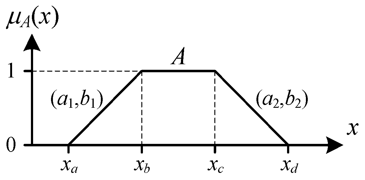
The graphical representation of the trapezoidal membership function ${\mu }_A\left(x\right)$ is shown in Figure 1.

Determining the value of the function is computationally demanding for the ranges $x_a<x<x_b$ and $x_c<x<x_d$. In these cases, calculating the function value requires subtraction and division operations [8,9]. Assume that all values in (2) are represented by n-bit binary numbers. While the normalized range of membership values is $[0,1]$, in binary logic, it is represented by the range $[0,2^n-1]$. Thus, Formula (2) must be additionally multiplied by the factor $2^n-1$ [10].

Assume that all values involved in the computation (n-bit parameters, arguments, and function values) are n bits in length. Calculating the trapezoidal membership function values involves several steps, where multiplication and division are the most computationally expensive operations [11,40,41]:

• Subtract the values in the numerator (n-bit value from n-bit value; the result is n bits long).
• Multiply the numerator by the factor $2^n-1$ (n-bit value by n-bit value; the result is $2n$ bits long).
• Subtract the values in the denominator (n-bit value from n-bit value; the result is n bits long).
• Divide the numerator by the denominator ($2n$-bit value by n-bit value; the result is n bits long).

The pseudocode for computing the membership function value for an input $x^{\prime }$ is presented in Algorithm 1. The code utilizes several variables to store data: the membership function parameters ($x_a,x_b,x_c,x_d$), the input value ($x^{\prime }$), and the computation result ($mbf$). For simplicity, ${\mu }_A\left(x\right)$ is denoted by $mbf$. While all of these variables store n-bit values, the length of auxiliary variables used for intermediate results can be greater, reaching $2n$ bits as described above [12,13].

Algorithm 1. Pseudocode for membership function computation based on parameters $(x_a,x_b,x_c,x_d)$.

1: if $((x^{\prime }<=x_a)$ or $(x^{\prime }>=x_d))$ then 2:     return 0 3: else if (($x^{\prime }>x_a$) and ($x^{\prime }<x_b$)) then 4:     return $((2^n-1)·(x^{\prime }-x_a))/(x_b-x_a)$ 5: else if $((x^{\prime }>x_c)$ and $(x^{\prime }<x_d))$ then 6:     return $((2^n-1)·(x_d-x^{\prime }))/(x_d-x_c)$ 7: else 8:     return  $(2^n-1)$ 9: end if

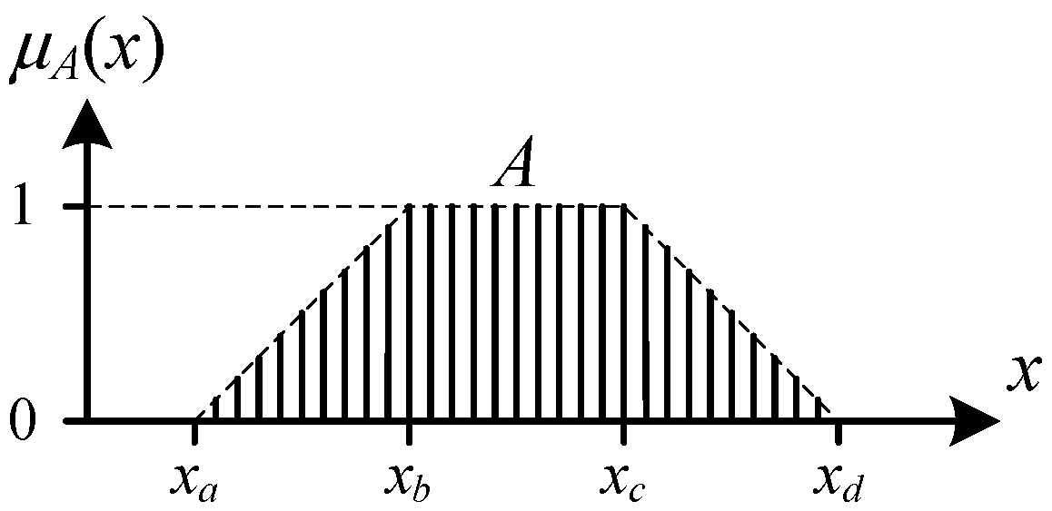
The computation steps should follow this order to achieve the best resolution (specifically step 2, which allows for avoiding fractional numbers). To avoid these operations during the inference process, the membership function can be precomputed, with the resulting values stored in a look-up table [42], as shown in Figure 2.

In this case, the memory size is $n·2^n$ bits and grows exponentially with the value of n. For example, if $n=8$, the memory size is 2048 bits; however, for $n=16$, it increases to as many as 1,048,576 bits [14,43]. As mentioned in Section 1, the memory footprint can be reduced by applying various data compression techniques, along with all associated consequences (such as increased overhead related to real-time decompression).

3. Bisection Algorithm

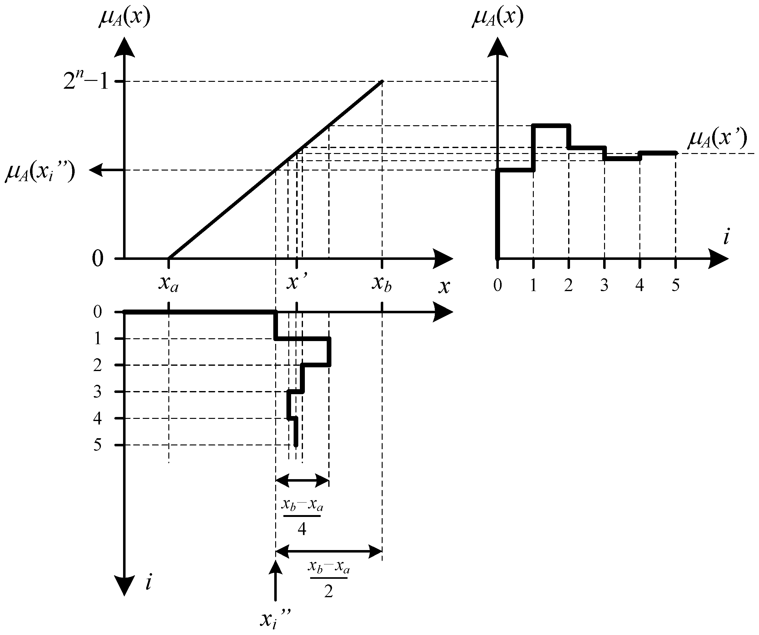
Multiplication and division operations are unnecessary to compute the membership function value if the modified bisection method (also known as the dichotomy method or the interval halving method) is used [12,13]. Let us consider the continuous and linear membership function ${\mu }_A\left(x\right)$ in the interval $[x_a,x_b]$, as shown in Figure 3, where the method is presented graphically (the ongoing considerations can also be extended to the interval $[x_c,x_d]$).

The figure illustrates the computational steps for determining the membership value ${\mu }_A\left(x^{\prime }\right)$ for a specific input $x^{\prime }$ [10]. The left and bottom graphs demonstrate how the membership value and the x value change over time during successive iterations [5].

Each i-th iteration of the bisection algorithm involves the following steps:

• Calculate the interval offset: ${\Delta }_{x_i}=(x_b-x_a)/2^{i+1}$.
• Determine the candidate value: $x_i^{″}=x_{i-1}^{″}\pm {\Delta }_{x_i}$ (where $x_0^{″}=x_a$).
• Compare the candidate value with the input: if $x_i^{″}>x^{\prime }$, then the next adjustment will be negative.
• Check for convergence: if the desired precision is reached (after n iterations), proceed to step 5; otherwise, return to step 1.
• Assign the corresponding membership value ${\mu }_A\left(x_i^{″}\right)$ based on the binary search progress.
• Return the final value ${\mu }_A\left(x^{\prime }\right)$ and terminate the process.

The classic bisection algorithm typically operates on real numbers [12,13]. Let us now assume that all values in the algorithm are represented by n-bit integers, and the membership values fall within the range $[0,2^n-1]$. Under these assumptions, the calculations in the primary algorithm can be significantly simplified [8,10].

First, in step 1 of the Algorithm 1, the division operation can be replaced by a binary right-shift by one bit in each iteration.

Second, steps 2 and 3 can be merged to avoid using signed integers. It is well known that calculations with signed numbers are more complex than those with unsigned ones. The new value $x_i^{″}$ is determined as $x_a+{\Delta }_{x_i}$ or $x_a-{\Delta }_{x_i}$, depending on the result of the comparison between $x_i^{″}$ and $x^{\prime }$.

Third, computing the membership function value ${\mu }_A\left(x_i^{″}\right)$ at point $x_i^{″}$ typically requires Formula (2), involving division and multiplication operations. However, for a linear function, the membership value can be updated within the main loop (steps 1 and 2) in each iteration using the method of successive approximation. In step 1, the interval midpoint for the membership function is calculated as ${\Delta }_{mbf}=2^n/2^{i+1}$, where the division is replaced by a binary right-shift by one bit in each iteration. Notably, an n-bit value shifted by n bits becomes zero; for example, ${\Delta }_{mbf}$ reaches zero after n iterations. In step 2, the current membership value is updated by adding or subtracting ${\Delta }_{mbf}$, depending on the comparison between $x_i^{″}$ and $x^{\prime }$.

Fourth, instead of checking the relationship between $x_i^{″}$ and $x^{\prime }$, it is more efficient to verify whether ${\Delta }_{mbf}$ has reached zero. Furthermore, the interval $[x_a,x_b]$ is not constant and may vary depending on the defined shape of the membership function. For small intervals, this variation may lead to a decrease in the accuracy of the computed function value.

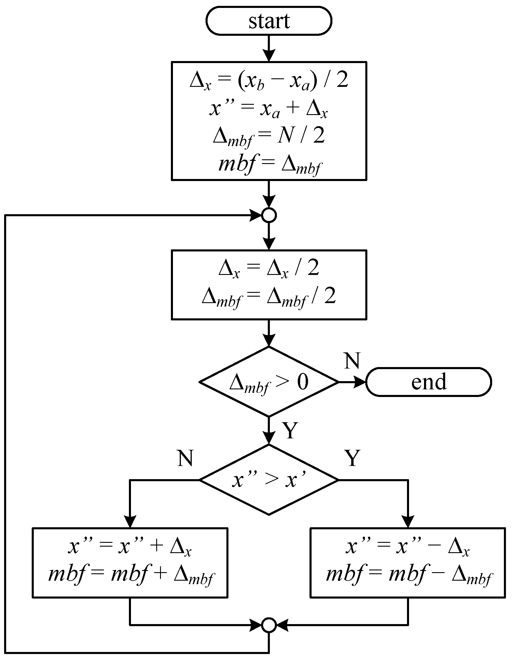
The block diagram of the algorithm for computing the function value, incorporating the proposed changes, is presented in Figure 4. The division by 2 is performed as a binary right-shift of the argument by one bit.

The pseudocode for computing the membership function value for a specific input $x^{\prime }$ within the interval under consideration is presented in Algorithm 2.

Algorithm 2. Pseudocode for computing the membership function value defined by parameters $(x_a,x_b)$ in the interval $x_a\le x\le x_b$.

1: ${\Delta }_x\leftarrow (x_b-x_a)\gg 1$   2: $x^{″}\leftarrow x_a+{\Delta }_x$   3: ${\Delta }_{mbf}\leftarrow 2^n\gg 1$   4: $mbf\leftarrow {\Delta }_{mbf}$   5: while ${\Delta }_{mbf}>0$  do   6:     ${\Delta }_x\leftarrow {\Delta }_x\gg 1$   7:     ${\Delta }_{mbf}\leftarrow {\Delta }_{mbf}\gg 1$   8:     if $x^{\prime }>x^{″}$ then   9:         $x^{″}\leftarrow x^{″}+{\Delta }_x$ 10:         $mbf\leftarrow mbf+{\Delta }_{mbf}$ 11:     else 12:         $x^{″}\leftarrow x^{″}-{\Delta }_x$ 13:         $mbf\leftarrow mbf-{\Delta }_{mbf}$ 14:     end if 15: end while

The expression $A\gg b$ denotes a binary bitwise right-shift of argument A by b bits, whereas $2^n$ represents 2 to the power of n.

It should be noted that in the first block of the algorithm (Figure 4) and in the Algorithm 2 (lines 1–4), i.e., at the initialization stage, complex multiplication and division operations do not occur. Instead, only operations of division by 2 (reduced to shifting the value by 1 to the right), summation, and copying are present. This is similar to what takes place during the actual evaluation of the function value in the loop (the remaining blocks of the algorithm while in the loop).

4. Implementations

The proposed algorithm was implemented as a fuzzy inference system module in both software and hardware. It was practically tested in an exemplary embedded system based on a general-purpose microcontroller and a field-programmable gate array (FPGA) [42].

The presented implementations compare the classical and proposed methods for computing membership function values. To ensure a fair evaluation of the discussed solutions, which perform the same function but are implemented using different techniques, the compared implementations must utilize the same underlying component library. For software implementations, this requires using the same processor/microcontroller instruction set, whereas for hardware implementations, it mandates employing solely general-purpose logic resources—namely, Look-Up Tables (LUTs) and flip-flops. Incorporating auxiliary components into either solution (such as multiplication and division instructions in software, or dedicated hardware multipliers and DSP modules in hardware) would compromise the comparison by favoring one approach over the other. Consequently, this would necessitate the introduction of advanced result normalization or correction factors. These measures would allow for separating the intrinsic efficiency of the algorithm architecture itself from the performance gain resulting exclusively from the technological characteristics of the hardware accelerators used (including those executing complex operations within the processor and expanding its instruction set, or DSP blocks and multipliers within the FPGA/ASIC fabric). The classical methods utilize standard mathematical operators for unsigned integers defined in the standard library (C implementation) or classical algorithms implemented in hardware or assembly [11]. For the division operation, the non-restoring division algorithm was used, while multiplication by a constant was replaced by bitwise shift operators [8,10].

To ensure a fair evaluation of the discussed solutions, experimental platforms with significantly more modest resources than those currently available on the market were utilized. The test programs employed the classic instruction set of the AVR microcontroller family (which lacks a division instruction), whereas the hardware modules were designed solely based on foundational logic—namely, LUT cells and flip-flops. This approach prevented hiding costly computations within the microcontroller’s machine code or inside dedicated blocks of the FPGA fabric. Furthermore, solutions based on such a basic resource set are fully portable to other platforms, and their performance parameters will only change quantitatively rather than qualitatively.

The software implementation was developed for an 8-bit Microchip AVR microcontroller (ATmega32 at a 16 MHz clock frequency) [4]. The embedded software was written in Assembly and C using the Microchip Studio (v7.0.2594) environment and the AVR 8 bit GNU Toolchain (v3.6.2.1778) with the AVR-GCC compiler (v5.4.0) [40,41].

The C code was compiled using AVR-GCC with the -Os optimization flag. The program memory (Flash) requirements were quantified based on compilation reports by analyzing the start and end addresses of the code segment, taking into account any subroutine calls. The program execution time, expressed both in clock cycles and microseconds, was determined using the cycle-accurate software simulator integrated into the Microchip Studio environment.

For the hardware modules described in Verilog, the synthesis and implementation processes were performed within the Xilinx ISE 8.2i environment [43,44] using the default optimization strategy settings, targeting the Xilinx Spartan-3 (XC3S200-4ft256) FPGA [2]. Hardware resource utilization was extracted directly from the post-mapping report (Map Report), accounting for the number of occupied Slices, Look-Up Tables (LUTs), and Flip-Flops. The estimated maximum clock frequency was obtained from the detailed synthesis report; based on this value, the final execution time was calculated as the product of the number of clock cycles required to complete the operation and the clock period (evaluated for both the maximum estimated frequency and a predefined reference of 100 MHz).

Both algorithms were tested with various data sizes: 8-bit, 16-bit, and a configuration with an 8-bit function value and a 16-bit argument. For the software implementation, the results are summarized in

Table 2. Implementation parameters for computing the membership function on an AVR microcontroller (8-bit data).

Implementation	Classic Algorithm		Bisection Algorithm
Parameters	Assembly	GCC	Assembly	GCC
Memory [B]	32	116	22	31
Speed [cycles]	258	264	98	100
Speed [μs] 1	16.1	16.5	6.1	6.3

¹ for clock frequency 16 MHz.

,

Table 3. Implementation parameters for computing the membership function on an AVR microcontroller (16-bit data).

Implementation	Classic Algorithm		Bisection Algorithm
Parameters	Assembly	GCC	Assembly	GCC
Memory [B]	46	238	42	62
Speed [cycles]	643	712	291	282
Speed [μs] 1	40.2	44.5	18.2	17.6

¹ for clock frequency 16 MHz.

and

Table 4. Implementation parameters for computing the membership function on an AVR microcontroller (16-bit input arguments and 8-bit membership values).

Implementation	Classic Algorithm		Bisection Algorithm
Parameters	Assembly	GCC	Assembly	GCC
Memory [B]	43	186	32	52
Speed [cycles]	466	661	250	250
Speed [μs] 1	29.1	41.3	15.6	15.6

¹ for clock frequency 16 MHz.

, and for the hardware implementation in

Table 5. Implementation parameters for computing the membership function on an FPGA (8-bit data).

Parameters	Algorithm
	Classic	Bisection
Number of Slice Flip Flops	30	32
Number of 4-input LUTs	56	52
Number of Slices	36	32
Total equivalent gate count	750	727
Maximum Frequency [MHz]	170	128
Computation time [ns] 1	94.1	62.5
Computation time [ns] 2	170	90

¹ for maximum frequency. ² for clock frequency 100 MHz.

,

Table 6. Implementation parameters for computing the membership function on an FPGA (16-bit input arguments and 8-bit membership values).

Parameters	Algorithm
	Classic	Bisection
Number of Slice Flip Flops	47	48
Number of 4-input LUTs	107	92
Number of Slices	61	52
Total equivalent gate count	1360	1215
Maximum Frequency [MHz]	154	108
Computation time [ns] 1	155.8	148.1
Computation time [ns] 2	250	170

¹ for maximum frequency. ² for clock frequency 100 MHz.

and

Table 7. Implementation parameters for computing the membership function on an FPGA (16-bit data).

Parameters	Algorithm
	Classic	Bisection
Number of Slice Flip Flops	55	64
Number of 4-input LUTs	107	105
Number of Slices	65	64
Total equivalent gate count	1424	1469
Maximum Frequency [MHz]	154	107
Computation time [ns] 1	207.8	149.5
Computation time [ns] 2	330	170

¹ for maximum frequency. ² for clock frequency 100 MHz.

.

It can be observed that the software implementation of the bisection algorithm achieves a significant reduction in both resource consumption (specifically program memory size) and computation time. These improvements are consistent across different programming languages and data sizes.

On the basis of the gathered data in Table 2, Table 3 and Table 4, it can be said that the description of the algorithm in assembler code leads to a reduction in memory size by 72–81% (classic algorithm) and 29–38% (bisection algorithm). The time of computing the result is comparable in the case of bisection algorithm, while for the classical algorithm one can notice its reduction by 2–30%.

Comparing the proposed algorithm with the classical one, three main conclusions can be drawn. First, the program memory size is reduced by 9–31% for the assembly code and 72–74% for the C code. Second, while the program size depends strongly on the data type in the assembly implementation, the proposed method remains more resource-efficient. Finally, the result is calculated 46–62% faster, and the performance is nearly independent of both the data type and the programming language used.

In the case of hardware implementation, the differences in hardware cost are insignificant, ranging from −3% to 11% (see Table 5, Table 6 and Table 7). This might initially suggest that this approach is not advantageous. However, the primary benefit is the significant reduction in computation time. The computation time is reduced by 32–48% when assuming a constant clock frequency (e.g., 100 MHz) and by 5–34% when comparing the maximum clock frequencies of each system.

It can be observed that for the module implementing the bisection algorithm, there was a decrease in the maximum clock frequency of the FPGA device compared to the classical solution (even though the computation time remains more favorable for the bisection algorithm). This effect could have been caused by the occurrence of a critical path; removing this critical path could increase the frequency and further reduce the evaluation time. This can be achieved by introducing pipelining or using alternative synthesis tools (e.g., Vivado, Quartus) that can automatically perform register retiming inside the combinational logic to balance propagation delays. During the testing phase, such a solution was not pursued in order to avoid introducing additional components, and the scope was restricted solely to the basic implementation of the bisection algorithm presented in Section 3.

Due to the approximate computation of the ${\Delta }_x$ value (Figure 4), where division operation is performed via bitwise shifting and omitting the least significant bit (LSB), a limited computation accuracy must be considered.

To evaluate this effect, a comparative analysis was conducted between the classical and the proposed algorithms within the fixed-point domain. The values obtained from the classical algorithm, derived directly from the exact analytical Formula (2), were adopted as the reference baseline.

The error evaluation methodology was structured as a two-stage process. First, partial errors were determined for all discrete points within a specific interval width ($x_b-x_a$). Subsequently, these partial values were aggregated across all analyzed intervals to compute the global Mean Absolute Error (MAE) and Root Mean Square Error (RMSE) indicators. To quantify the overall numerical degradation, these metrics were calculated for 8- to 12-bit representations of ${\Delta }_x$.

The analysis covers the entire range of variations for the $(x_b-x_a)$ interval width. The results are summarized in

Table 8. Comparison of MAE and RMSE errors based on interval width.

Error Metrics	8 Bits	9 Bits	10 Bits	11 Bits	12 Bits
MAE	1.89	0.92	0.61	0.51	0.49
RMSE	3.07	1.51	0.93	0.75	0.71

.

As the computational resolution increases, the accuracy of calculating the membership function value (encoded in 8 bits) increases, while the MAE and RMSE errors systematically decrease. For the 8-bit resolution, the error is greatest (MAE = 1.89, RMSE = 3.07) because fewer bits represent data with lower resolution, which limits calculation precision. The best results are achieved for 12 bits, where the mean absolute error (MAE) drops to 0.49, representing only a 0.19% error for the full range of membership function values. Notably, the greatest reduction in error occurs when switching from 8 to 9 bits, with a decrease in MAE by 0.97 and a decrease in RMSE by 1.56.

Notable numerical anomalies are observed across all analyzed bit resolutions, with RMSE values systematically exceeding the corresponding MAE metrics. Within statistical error analysis, this trend clearly demonstrates that, regardless of the computational resolution, the algorithm is subject to isolated large errors, even though their magnitude drastically diminishes as the resolution increases (with RMSE dropping from 3.07 to 0.71).

These peak errors represent a core limitation of the proposed method; they reach their maximum values exclusively for narrow widths of the $x_b-x_a$ interval that are not aligned with power-of-two boundaries (when the interval widths are exact powers of two, the computation proceeds without any loss of precision, yielding an error of exactly zero).

In fuzzy inference systems, typically 3 to 7 membership functions are applied per single linguistic variable [45]. In such cases, the interval widths are typically 30 or more. Only in certain situations are membership functions clustered more densely in regions where the system requires the highest operational precision [46], which consequently reduces the width of that interval. In the case of very narrow intervals, where error values may become significant, the interval boundary points can be slightly shifted to achieve an interval width that is a power of 2. Fuzzy systems are characterized by an inherent robustness to disturbances and parametric errors [47]. A minor modification to the boundaries of the membership function shape (e.g., expanding the support, i.e., the interval width, from 30 to 32) will cause a minimal, smooth variation in the control surface, which generally does not affect the system behavior or stability.

Due to the difficulties in analytically generalizing the impact of membership function shape variations on systems with diverse knowledge bases, the final verification of operational correctness requires conducting simulation studies or real-world testing [48].

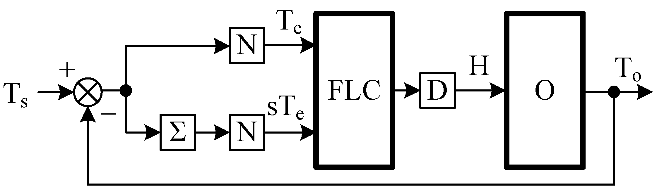
In situations where the interval width cannot be freely chosen, it is necessary to evaluate the influence of the proposed algorithm on the behavior of the entire fuzzy inference system in a practical application. The impact of using the bisection algorithm for membership function computation was tested using a fuzzy PI controller (FLC) within the real-world temperature control system shown in Figure 5.

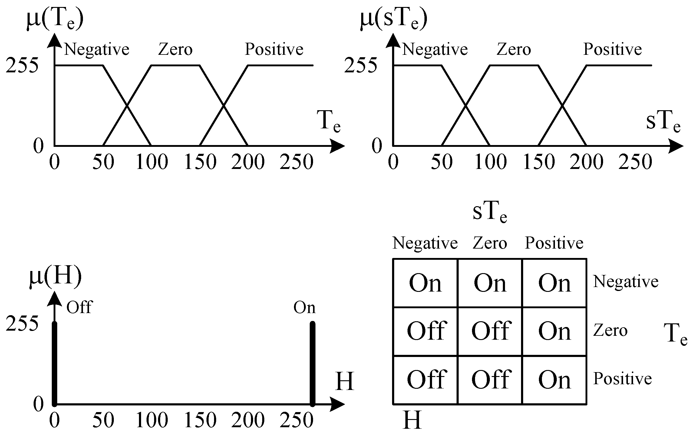
Modules denoted as N and D are used for the normalization and denormalization of physical quantities to the range $[0,2^n-1]$ required by the FLC. The ∑ module performs the integration of the input signal, which is the temperature error $T_e$. The controlled object consists of a heat sink heated by a resistor. The behavior of the fuzzy logic controller is defined by the knowledge base shown in Figure 6.

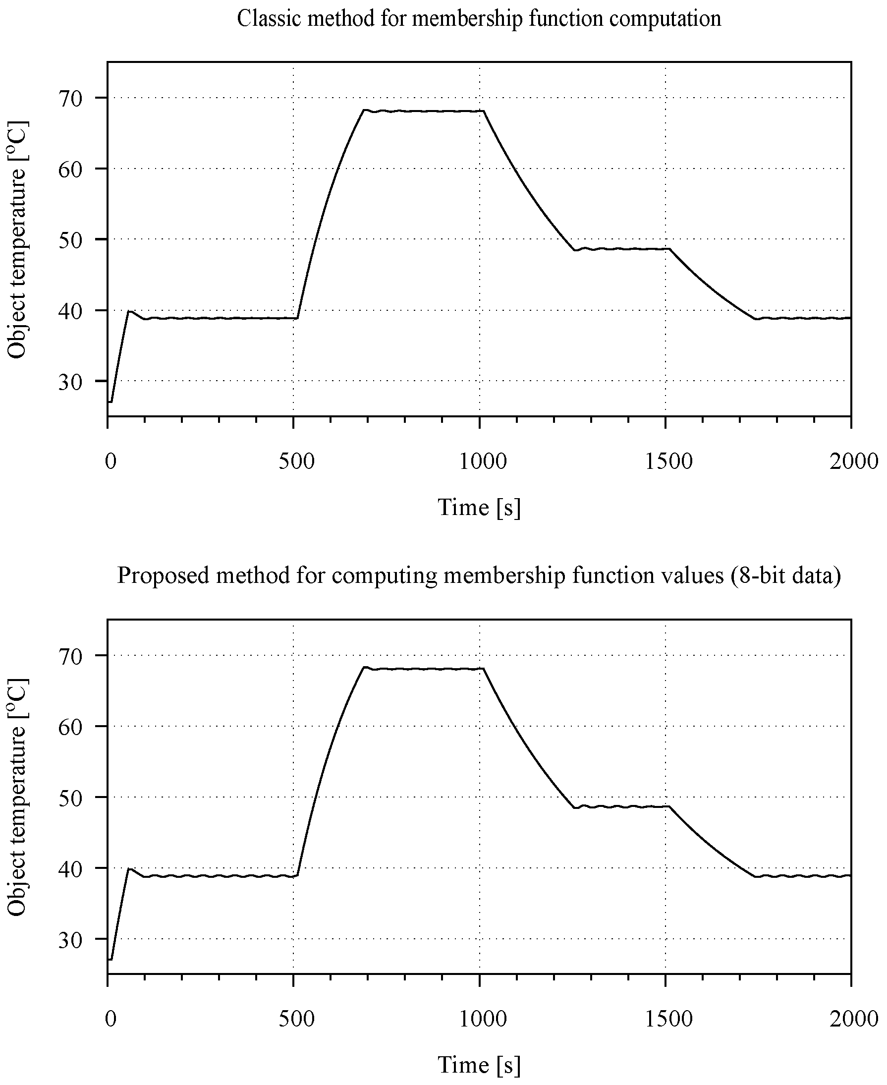
Timing diagrams of the system’s key parameters (specifically the object temperature) for both the classical and bisection algorithms are presented in Figure 7.

As can be seen in this example, with a computation error of the membership value not exceeding 2%, only minor changes in the control system’s behavior were observed. A slight increase in the overshoot (approximately 0.5%) and the settling time can be noted.

5. Conclusions

The proposed modified bisection method serves as an efficient alternative for embedded fuzzy inference systems, specifically targeting the microcontrollers and programmable logic devices (FPGAs) that lack dedicated hardware multipliers and dividers. By replacing complex arithmetic operations with basic addition and bitwise shifts during both the initialization and execution phases, the method provides several critical advantages:

• While both the classical and the proposed methods offer predictable latency, the proposed approach achieves a shorter execution time under the tested conditions, suggesting its potential suitability for specific real-time embedded applications.
• The proposed approach significantly reduces memory usage, since the functions require storing only a few node coordinates rather than extensive arrays, as is typical for standard look-up tables (LUTs). Moreover, any nonlinear curve can theoretically be approximated with satisfactory accuracy by utilizing an appropriately selected number of linear segments.
• Reducing the execution time required to compute the function value enables the potential minimization of the system’s dynamic power consumption.
• The hardware implementation is based on general-purpose programmable logic (standard LUTs and flip-flops) without the mandatory utilization of specialized DSP blocks or hardware multipliers, thereby keeping these resources available for other tasks in a design. By avoiding vendor-specific hardblocks, the Verilog description exhibits high portability across different FPGA architectures (such as AMD/Xilinx or Intel/Altera) and simplifies the potential migration pathway to ASIC implementations.
• The software implementation utilizes a basic instruction set and can be executed across various architectures. It is particularly suited for severely resource-constrained systems, such as low-cost microcontrollers lacking a hardware division unit. Although the algorithm can also be deployed on high-performance platforms, it will not yield such significant performance improvements in those cases.
• The accuracy of the computed outcome, even for the adopted 8-bit resolution, proved satisfactory during the experimental validation on the actual hardware and may be sufficient for a selected class of practical fuzzy logic applications.

Based on the experimental results and implementation analysis, the following conclusions can be drawn.

First, the proposed algorithm significantly reduces the computational load by replacing complex multiplication and division operations with simple binary shifts and additions. In software implementations, this approach resulted in a 46–62% reduction in computation time and a significant decrease in program memory usage, particularly for C-based developments.

Second, hardware implementations on FPGA devices demonstrated that while the logic resource consumption remains comparable to classical methods, the bisection algorithm offers a substantial speed advantage. When operating at a constant clock frequency, the proposed method is 32–48% faster, making it highly suitable for high-speed control applications.

Finally, experimental tests on a real-world temperature control system with a fuzzy PI controller confirmed the practical viability of the method. Even with the limited accuracy inherent in fixed-point bisection, the impact on control quality—specifically overshoot and settling time—was negligible. Thus, the proposed method is an efficient alternative for resource-constrained embedded systems where performance and memory efficiency are critical.