Article

A Drift-Aware Human-in-the-Loop Edge AI Agent for Wireless IoMT Sensor-Network Intrusion Detection Under Cross-Corpus Shift

by
Abdulaziz Saleh Alajaji
Department of Information Systems, College of Computer and Information Sciences, King Saud University, Riyadh 11543, Saudi Arabia
Electronics 2026, 15(14), 3015; https://doi.org/10.3390/electronics15143015
Submission received: 12 June 2026 / Revised: 4 July 2026 / Accepted: 7 July 2026 / Published: 9 July 2026
(This article belongs to the Section Networks)

Abstract

Wireless sensor networks underpin the Internet of Medical Things (IoMT), where connected medical devices and wearable body-area sensors stream patient telemetry across hospital networks, and securing this traffic is safety-critical. Machine learning intrusion-detection systems for the IoMT are usually evaluated within a single public dataset, where they report near-perfect detection scores; whether that accuracy predicts performance in a different hospital has not been measured systematically. We frame the deployed detector as a lightweight human-in-the-loop edge AI agent that observes local traffic, asks an analyst to label a small set of representative flows, trains a tiny model on-premises, and monitors the traffic distribution for drift. Using cross-corpus shift across four public datasets, comprising three sensor-network corpora (WUSTL-EHMS-2020, CIC-IoMT-2024, TON-IoT) and an unrelated enterprise-network corpus, as a reproducible stand-in for cross-hospital deployment, we find the shift is near its theoretical maximum on all twelve transfer directions, that unlabeled domain-adaptation methods collapse on the hardest medical-telemetry targets, and that external pretraining adds no measurable benefit once training schedules are matched, consistent with a domain-adaptation error bound that the measured divergence renders vacuous. The same 1206-parameter network trained from scratch on ten to fifty locally labeled flows matches or exceeds every transfer alternative across all four corpora; on the six sensor-network transfer directions it also outperforms larger and classical local models. A closed-loop evaluation on simulated drifting streams shows the calibrated trigger detects drift within two 500-flow windows at under one false alarm per hundred stationary windows, retraining restores accuracy, and the agent tolerates ten percent analyst error for about five F1 points; we also map the detector’s exposure to white-box evasion and targeted label poisoning.

1. Introduction

The Internet of Medical Things (IoMT) extends wireless sensor network (WSN) and body-area-network technology into clinical settings, integrating connected medical devices (patient monitors, infusion pumps, wearable sensors, and imaging equipment) into hospital networks, and has become a primary surface through which cyber-attacks reach clinical care [1,2]. Because compromised medical-device telemetry can directly affect patient safety, network intrusion detection for the IoMT sensor subnet is an operational priority rather than a purely academic one.
IoMT and wearable-health systems increasingly rely on cloud-edge AI architectures that distribute intelligence across sensing devices, gateway nodes, and cloud services to balance responsiveness, communication cost, privacy, and scalability [3]. Within this architecture, the line of work on resource-efficient inference shows that constrained edge devices benefit from lightweight deployment strategies such as model compression and quantization [4] and edge-cloud partitioning of inference [5]. Our detector sits at the gateway end of this spectrum: it is a 1206-parameter model ( 4.7  KB, sub-millisecond inference per thousand flows; Table 1) that runs entirely on-premises, so it inherits the latency, energy, and privacy advantages those strategies’ target without an offloading step. The footprint is at or below that of prior lightweight gateway-resident IoMT/IoT IDS such as Passban [6], which we treat as the reference class for edge-deployable detection. Unlike general deployment-optimization studies, the present work focuses on whether such an on-gateway detector should be obtained by importing and adapting an external public-corpus model or by training a fresh local model, and on keeping it reliable under distribution drift.
The workflow targets resource-constrained IoMT gateways, where flow-level telemetry must be processed locally with a compact model, limited labeling, and no cross-institutional telemetry export [6]. Machine learning network intrusion-detection systems (IDSs) for IoMT report within-corpus F 1     1.0 on public benchmarks [7,8,9], implicitly assuming that within-corpus performance predicts deployment performance. This assumption has not been measured systematically, because IoMT IDSs evaluation is, with few exceptions, single-corpus: a model is trained and tested on splits of the same capture, so the reported number reflects in-distribution generalization rather than the cross-environment generalization a real deployment demands.
A hospital deploying an IoMT IDS realistically chooses between two options: use a public-corpus pretrained model (possibly adapted with standard domain-adaptation tooling) or have the local IT team label a small batch of in-house flows and train a model from scratch. Intuition favors the first option: pretraining on hundreds of thousands of labeled flows ought to dominate hand-labeling fifty. However, if public IoMT corpora differ enough in capture methodology, attack taxonomy, and feature schema, a small from-scratch model trained on in-distribution labels may suffice, and the operational and regulatory cost of importing an external model may not be repaid by any accuracy gain. We measure this question across four public IDSs corpora-harmonized onto a common nine-feature flow schema, using cross-corpus shift as a publicly reproducible proxy for cross-hospital deployment shift. Three are sensor-network captures: WUSTL-EHMS-2020 [7] and CIC-IoMT-2024 [8] for medical IoMT, and TON-IoT [10] for broader IoT/IIoT traffic. The fourth, CSE-CIC-IDS-2018 [11], is an enterprise-network corpus from an unrelated capture that carries the audit beyond the medical domain and rules out any dependence on a single capture lineage. The gap between this cross-corpus proxy and true cross-hospital deployment is examined in Section 9. We organize the study around three research questions:
  • RQ1. How large is the distribution shift across the evaluated corpus pairs, especially the primary WUSTL ↔ CIC IoMT pair? We measure it directly with the H-divergence proxy [12] and a kernel maximum mean discrepancy (MMD) [13].
  • RQ2. To what extent do canonical cross-corpus adaptation methods recover target-domain F 1 under severe shift? We evaluate eight adaptation methods spanning labeled, unlabeled, and source-free regimes.
  • RQ3. How does direct local-supervised training, a tiny model trained from scratch on a small in-house labeling budget, compare with cross-corpus adaptation across target-label budgets N?
With the transfer question settled, we turn to deployment and characterize how the recommended workflow behaves under alternative model classes, feature masking, white-box evasion, targeted label poisoning, and competing drift triggers (Section 7 and Section 8).
Findings. (RQ1) The shift is essentially maximal on every pair: a domain classifier tells the corpora apart perfectly, and the H-divergence proxy saturates while the kernel MMD stays consistently large (Section 6). (RQ2) On the directions whose target is the medical-telemetry corpus, every unlabeled method (DANN, Deep CORAL, TENT, pseudo-labeling, and plain source-only transfer) stays below an F 1 of 0.22 , consistent with the theoretical lower bound on marginal-alignment adaptation under conditional shift [14]; easier directions retain partial utility. (RQ3) Once fine-tuning schedules are matched, source pretraining is statistically indistinguishable from training the same model from scratch on the local labels. In this severe-shift setting, training the tiny model from scratch on representative target labels provides the same practical benefit as importing and adapting an external source model.
This paper is a deployment audit of a constrained edge AI-agent workflow: the tiny model avoids dependence on source labels and source model weights, cross-institutional data sharing, and adaptation-pipeline complexity while matching the target-domain performance of more complex alternatives.
The novelty is not a new learning algorithm; the components (a small MLP, k-medoids selection, MMD drift detection, and detect-then-retrain looping) are individually standard. Three elements distinguish this work from prior human-in-the-loop and edge-AI IDS research. First, existing human-in-the-loop and active-learning IDS studies assume a single corpus and ask how few labels recover within-corpus accuracy; we instead measure the deployment decision itself, quantifying when a small local labeling round is preferable to importing and adapting an external model under measured cross-environment shift. Second, prior edge-AI IDS work optimizes the on-device model in isolation; we tie the model to a closed loop in which a calibrated, label-free drift trigger decides when the human-in-the-loop step is re-invoked, and we validate that loop end-to-end on drifting streams against standard drift detectors. Third, we connect the empirical outcome to domain-adaptation theory, showing that the measured separability drives the transfer bound to a vacuous value, which explains rather than merely reports the negative transfer result. The contribution is therefore this audit, the closed-loop workflow, and the theoretical framing, not a new adaptation mechanism. The contributions of this paper are as follows:
  • A reproducible cross-corpus deployment audit for lightweight IDS over four public corpora that span medical IoMT (WUSTL-EHMS-2020 [7], CIC-IoMT-2024 [8]), general IoT/IIoT (TON-IoT [10]), and enterprise networks (CSE-CIC-IDS-2018 [11]), all harmonized onto a common nine-feature flow schema. Across the twelve ordered transfer directions, the measured shift sits near its theoretical maximum, and the negative-transfer pattern is uniform across medical and non-medical captures.
  • Evidence that standard cross-corpus transfer and adaptation methods do not reliably survive this shift: unlabeled domain adaptation (source-only, DANN, Deep CORAL, TENT, pseudo-labeling, and the recent source-free method SHOT) is unstable across directions and collapses on WUSTL-target settings, while source pretraining followed by matched-schedule fine-tuning gives no measurable advantage over from-scratch target training. Every primary comparison is backed by paired, multiplicity-corrected tests over fifteen runs and a hyperparameter-fairness ablation.
  • A theoretical interpretation of the empirical collapse: the measured domain separability drives the domain-adaptation target-error bound to a vacuous value, which explains why marginal-alignment methods have little room to recover target-domain accuracy under the observed conditional shift.
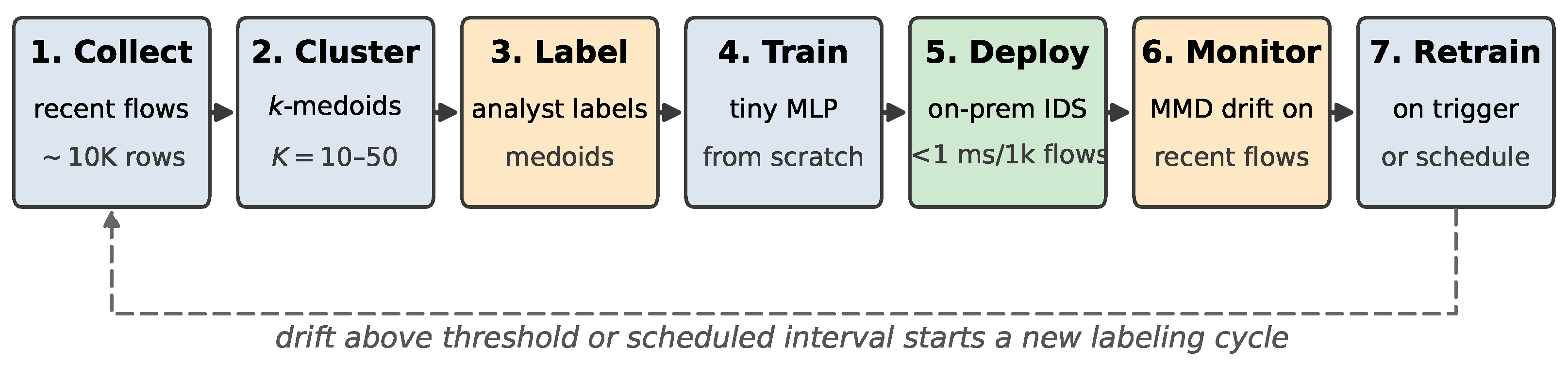
  • A constrained human-in-the-loop edge-agent workflow for IoMT IDS deployment, in which the agent observes recent local flows, summarizes them with k-medoids, requests analyst labels for representative medoids, trains a 1206-parameter classifier on-premises, monitors drift, and triggers retraining while keeping labeling authority with the human analyst.
  • A deployment-validation study of that workflow (architecture and feature ablations, analyst label-noise tolerance, targeted label poisoning, white-box evasion, and a comparison of drift triggers in closed loop on simulated drifting streams) that identifies the operating conditions under which the compact local model remains reliable and those under which the deployed agent remains vulnerable.
The remainder of this paper is organized as follows. Section 2 reviews single-corpus IoMT IDS evaluation, cross-dataset generalization, and domain-adaptation theory. Section 3 defines the constrained edge AI-agent deployment model, and Section 4 states the threat model and deployment scenario. Section 5 describes the corpora, harmonization, architecture, and statistical protocol. Section 6 quantifies the cross-corpus shift and interprets it through the domain-adaptation target-error bound. Section 7 reports the empirical results—the primary six-direction audit, budget curves, the full twelve-direction matrix over the four corpora, operational precision/recall trade-offs, architecture and feature ablations, active labeling, analyst label-noise tolerance, and adversarial robustness. Section 8 assembles the findings into the drift-aware agent workflow and compares drift-trigger alternatives in closed loop on simulated drifting streams. Section 9 discusses implications and limitations, Section 10 outlines future work, and Section 11 concludes.

2. Related Work

2.1. Single-Corpus Evaluation of IoMT and IoT Intrusion Detection

Surveys of IoMT and healthcare-system security identify network intrusion detection at the medical-sensor subnet as a core defense layer [1,2], and lightweight gateway-resident IDS designs such as Passban [6] demonstrate that anomaly detection can run directly on IoT edge hardware. On the evaluation side, Hady et al. [7] and Dadkhah et al. [8] introduced WUSTL-EHMS-2020 and CIC-IoMT-2024 with within-corpus headline F 1 0.99 each. The general IoT-IDS literature [9] similarly reports single-corpus evaluations, and broad IoT/IIoT benchmarks such as TON-IoT [10] are likewise typically used in a train-and-test-on-the-same-capture protocol. We are not aware of any prior cross-corpus IoMT IDS evaluation; existing IoMT IDS studies largely report within-corpus performance and therefore do not answer the deployment question addressed here—whether public-corpus transfer improves IDS performance under cross-corpus shift used as a public-corpus proxy for hospital deployment. The near-saturated single-corpus numbers are best read as in-distribution references rather than predictions of cross-environment behavior.

2.2. Cross-Dataset Generalization in Network Intrusion Detection

Outside IoMT, the limits of single-corpus evaluation are better documented. Sommer and Paxson [15] identified the gap between closed-world benchmark evaluation and operational network monitoring as the central reason machine learning IDS sees limited deployment, and Arp et al. [16] catalog the recurring pitfalls—including sampling bias and dataset artifacts—that inflate published detection results. Dataset-quality studies reinforce the point: Engelen et al. [17] document labeling and feature-extraction defects in the widely used CICIDS2017 corpus. Layeghy and Portmann [18] measured cross-dataset generalization for general network IDSs and reported large drops when models are moved between captures, and Apruzzese et al. [19] systematized the role of unlabeled data and the practical obstacles to deploying learning-based detectors in operational settings. These studies motivate treating cross-corpus transfer, rather than within-corpus accuracy, as the quantity of interest for deployment. Our work specializes this concern to the IoMT/smart-health setting and pairs it with an explicit comparison against a small locally trained model.

2.3. Unsupervised Domain Adaptation and Its Theoretical Limits

Standard domain-adaptation (DA) tools underpin our baselines: adversarial feature alignment via DANN [20], second-order feature-covariance alignment via Deep CORAL [21], and test-time batch-normalization adaptation via TENT [22], together with the broader feature-transfer and H-divergence framework [12,23,24]. The theoretical ceiling on these methods is equally relevant: the H-divergence bound [12] ties transferable risk to the distinguishability of the two domains, and Zhao et al. [14] prove a lower bound showing that marginal-feature alignment cannot guarantee target performance when the label-conditional distributions differ. We use the kernel MMD [13] as a complementary, classifier-free measure of marginal shift; the broader dataset-shift taxonomy is laid out by Quiñonero-Candela et al. [25]. More recent source-free domain adaptation, which adapts a source-trained model without access to the source data (for example, source-hypothesis transfer [26]), and test-time adaptation such as TENT [22] belong to the same marginal-alignment family: both adjust the model to the target marginal but cannot supply the target label-conditional information that the lower bound of Zhao et al. [14] shows is required, so the same theory anticipates limited headroom under the conditional shift we measure. We test this prediction directly: alongside TENT, we evaluate SHOT as a representative recent source-free method (Section 7.5), and both stay below direct local-supervised training on every direction. The temporal counterpart of cross-environment shift is concept drift, for which detection-and-retraining loops are the standard adaptation pattern [27,28]; our workflow instantiates that pattern at the IoMT gateway with a calibrated MMD trigger. As the results show, the negative outcome we measure is the empirical face of these bounds: when the domain classifier separates the corpora perfectly, marginal alignment has little room to help, and conditional shift does the rest.

2.4. Research Gap

The literature establishes that (i) IoMT IDS is overwhelmingly evaluated single-corpus, (ii) cross-dataset transfer degrades sharply for general network IDSs, and (iii) DA theory bounds what marginal alignment can recover under conditional shift. What is missing is a controlled, reproducible audit that places these threads together in the IoMT setting and asks whether a hospital is better served by importing and adapting an external model or by labeling a small local sample. This paper provides that audit and packages the answer as a deployable human-in-the-loop edge-agent workflow.

3. AI Agent Deployment Model

We model the deployed IDS as a constrained human-in-the-loop edge AI agent operating at the hospital IoMT gateway. The agent is constrained because it does not independently assign ground-truth security labels or autonomously change the hospital security policy. Instead, it automates four bounded functions: observing recent flow-level traffic, selecting representative flows for analyst labeling, training a compact local classifier, and monitoring post-deployment drift.
This framing separates automation from authority. The agent summarizes traffic, recommends which flows should be labeled, trains and deploys a tiny IDS model, and triggers a retraining request when drift is detected. The analyst, however, remains responsible for security-critical labeling decisions. This design is appropriate for smart-health environments, where medical-device telemetry is sensitive, cross-institutional data sharing is restricted, and fully autonomous adaptation may introduce unsafe model updates. The agent therefore occupies a middle ground between fully manual IDS maintenance, which scales poorly, and fully autonomous adaptation, which removes the human oversight that security-critical and safety-critical clinical environments require.

Formal Specification

We state the agent as a tuple ( O , S , A , π , ρ ) so that the automated and human-controlled steps are explicit. The observation space O is a sliding window W t R m × 9 of the m most recent flows on the harmonized nine-feature schema. The internal state S comprises the current classifier parameters θ t , the reference window W ref fixed at the last (re)training, and the calibrated drift threshold τ . The action set is A = {Monitor, Select, RequestLabels, Train, Deploy}. The agent’s policy π is deterministic and rule-based rather than learned: in the steady state it takes Monitor, computing the drift statistic d t = MMD ( W t , W ref ) ; when the trigger predicate ρ ( d t , τ ) = 1 [ d t > τ ] fires (or a scheduled interval elapses), the policy executes the bounded sequence SelectRequestLabelsTrainDeploy, where Select returns K medoid flows, Train fits θ from scratch on the analyst-provided labels, and  W ref is reset. The crucial restriction is that the label-assignment function that produces ground-truth y for the selected medoids is not part of π ; it is the human analyst, which is what makes the agent constrained rather than autonomous. The reward the policy implicitly optimizes is post-retraining target F 1 at the smallest analyst-labeling cost, and Section 7.8 and Section 8.1 measure both terms. Algorithm 1 below is the executable form of this specification.
Algorithm 1 Drift-aware human-in-the-loop IDS agent loop.
  1:
Input: traffic stream; labeling budget K; drift threshold τ
  2:
Collect a recent-traffic window W ( 10 K flows)
  3:
Standardize W to the harmonized nine-feature schema
  4:
M k - medoids ( W , K )                        ▹ representative flows
  5:
Analyst labels the medoids M                 ▹ human authority retained
  6:
Train the 9 32 16 2 MLP from scratch on ( M , labels )
  7:
Deploy the model for on-premises inference at the gateway
  8:
loop                          ▹ post-deployment monitoring
  9:
       d MMD(recent window, training window)
10:
      if  d > τ  or scheduled interval elapsed then
11:
           trigger retraining (return to line 2)
12:
      end if
13:
end loop

4. Threat Model and Deployment Scenario

A hospital IT team installs a binary attack/benign network IDS on its IoMT subnet, with access to (i) a public-corpus pretrained model (a vendor or research artifact), and (ii) the ability to label a small number of recent in-house flows by hand. The adversary is a network-layer attacker producing either medical-device data-stream attacks (WUSTL: spoofing or alteration of patient-monitor telemetry) or IoT-network volumetric attacks (CIC: DDoS, MQTT flood, ARP spoof, reconnaissance). We do not model an adversary that adapts to the IDS; we measure the static-attack regime that the public corpora capture. The defender has read access to one public corpus (source), unlabeled access to flows from the target deployment environment, and a labeling budget N { 10 , 50 , 200 , 500 , 1000 } . The assumption of a representative pool of unlabeled target flows is mild in this setting: a gateway-resident detector observes its own local traffic by construction, so collecting a recent-traffic window is a passive capture step that needs no labels, no external data, and no cross-institutional sharing. It is the labels on that traffic, not the traffic itself, that are scarce, which is exactly why the agent spends its budget on a small analyst-labeled medoid set. This scenario isolates the variable of interest—whether external source data help—while holding the detector architecture and labeling interface fixed.

5. Experimental Setup

5.1. Corpora and Harmonization

WUSTL-EHMS-2020 [7] contains 16 , 318 flows ( 87.5 % benign) with spoofing/alteration of patient-monitor telemetry; CIC-IoMT-2024 [8] contains ∼1.6M flows dominated by DDoS variants, balance-sampled to 20K+20K per seed; TON-IoT [10] contains ∼211K flows across nine IoT/IIoT attack families; and CSE-CIC-IDS-2018 [11] (CSE-IDS2018 in tables and figures) contributes an enterprise-network capture produced with a CICFlowMeter toolchain and a DoS, DDoS, Bot, Brute-Force, Infiltration, and Web attack taxonomy. The four corpora come from four unrelated captures and span medical IoMT, general IoT/IIoT, and enterprise traffic. WUSTL ↔ CIC is the primary smart-health/IoMT case study and carries the full statistical protocol; TON-IoT and CSE-IDS2018 extend the audit to general IoT and non-medical enterprise traffic and complete the twelve-direction matrix of Section 7.4.
The native schemas share no identical column names. We construct a manual semantic mapping (Table 2) onto a common nine-feature flow schema (rate, duration, inter-arrival time, total bytes, total packets, minimum/maximum/average packet size, and jitter); the CSE-IDS2018 column of Table 2 gives its CICFlowMeter mapping, drawn from a balanced benign/attack subset over its DoS, DDoS, Bot, Infiltration, and Web capture days under the same stratified 70 / 30 split per seed used for the other corpora. TON-IoT’s Zeek-style records carry no per-flow packet-size minima/maxima or jitter, so those three columns degenerate to the average packet size and zero, respectively; the harmonized vector therefore loses some discriminative information for TON-IoT while staying aligned with the other two schemas. Features are standardized via a quantile transformer fit on the union of source-train and target-unlabeled features; the same target-unlabeled snapshot is used for scaling in all methods to avoid pre-processing asymmetry. The target-unlabeled snapshot used for scaling and for unsupervised adaptation is the target train partition, which is disjoint from the target-test partition by the stratified 70 / 30 split; target-test labels are never used in pre-processing, training, model selection, or threshold calibration. Within-corpus references on the harmonized schema (the same 9 32 16 2 MLP, mean over 5 seeds) are WUSTL F 1 = 0.60 , TON-IoT 0.85 , CIC 0.996 , and CSE-IDS2018 0.98 , confirming that the interface is not broken on any corpus; harmonization on WUSTL costs ∼5 percentage points versus the 30-feature native schema (Random Forest, F 1 = 0.655 0.606 ), dominated by removing eight biometric features rather than by harmonization itself.

5.2. Architecture and Methods

We use a single 9 32 16 2 MLP (batch normalization + ReLU, 1206 parameters, 4.7  KB at float32) for all nine methods, so that differences in performance reflect the training regime rather than model capacity (The 1206-parameter count is sum(p.numel() for p in model.parameters()) over the full shared module, including the input batch-normalization affine parameters and the domain-discriminator head used by DANN; the classifier-only inference path (input BN, two hidden layers, and the two-way classifier head) accounts for 900 of these parameters). Six methods use no target labels (cross-corpus DA): source-only, DANN [20], Deep CORAL [21], TENT [22], pseudo-labeling, and the source-free method SHOT [26]. Two methods use N target labels on top of source pretraining: source-pretrain plus full-network fine-tune, and source-pretrain plus linear probe. The ninth is direct local-supervised training: train the same MLP from scratch on N labeled target flows using no source labels and no source model weights. For comparability with the transfer baselines, its quantile scaler is fit on the same source-train plus target-unlabeled features used throughout (Section 5); for strict source-free deployment the scaler can instead be fit on the local unlabeled target window alone, which removes the last dependence on source data. SHOT is evaluated across the full twelve-direction matrix (Section 7.5); the other eight methods are additionally evaluated across the six cross-corpus directions (Section 7.1).
These baselines are chosen to cover the canonical families of cross-corpus transfer rather than to be exhaustive: source-only is the no-adaptation lower bound; DANN represents adversarial feature alignment; Deep CORAL represents moment (covariance) matching; TENT and the more recent SHOT (Section 7.5) represent test-time and source-free adaptation; pseudo-labeling represents self-training; and source-pretrain plus fine-tune or linear probe represent the supervised-transfer references a deployer would actually try. Each is lightweight enough to run within the gateway envelope of Section 7.7, which is a deployment constraint that excludes heavier adaptation pipelines. Because every method shares one architecture and one labeled set, the comparison isolates the training regime; the domain-adaptation lower bound of Section 6.1 further implies that other marginal-alignment variants would face the same ceiling on the directions where these collapse.
Target-label selection. For the main N-label comparisons (Table 3 and Table 4, Figure 1), the N target labels are drawn by class-balanced stratified sampling from the target-train partition, and the identical labeled set is shared by all methods that consume target labels, so that differences reflect the training regime rather than the draw. Stratified selection isolates the transfer question from the selection question; Section 7.8 then separately compares random, stratified, uncertainty, and k-medoids selection policies and shows that the agent’s deployed k-medoids policy is the stronger choice on the hardest direction at small budgets. The class-balanced stratified draw is an analysis device, not a deployment assumption: it presumes knowledge of the target class proportions only so that the main grid varies the training regime and not the label mix. The deployed agent never uses this information. Its k-medoids selector is fully unsupervised, choosing representative flows from the covariate distribution alone, and Section 7.8 shows that at B = 10 it already exceeds on the hardest direction the F 1 that the balanced stratified draw reaches at N = 50 , so the headline finding does not rest on the balance assumption.
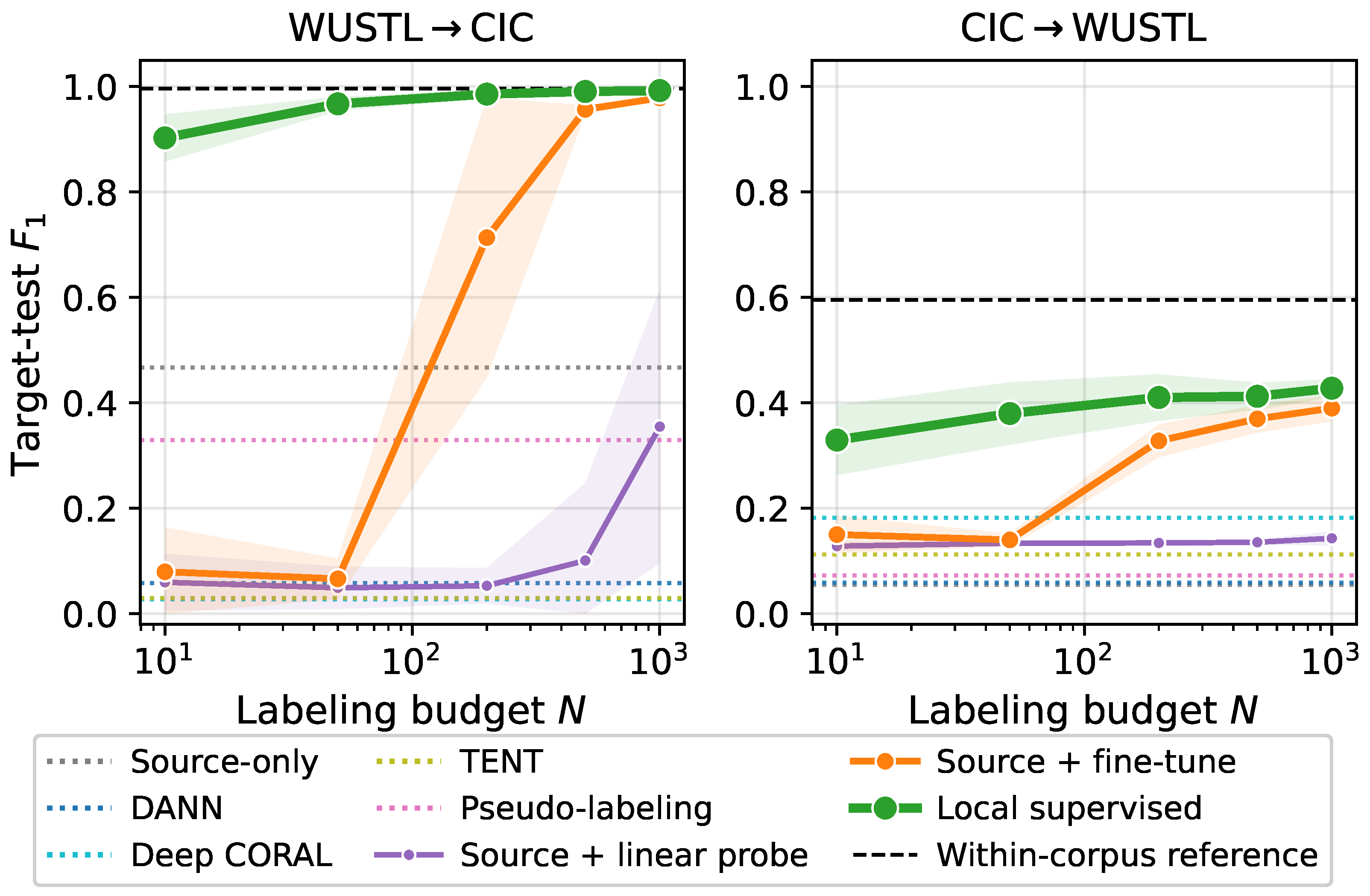
Figure 1. Target-test F 1 versus labeling budget N on the primary WUSTL ↔ CIC pair (5 seeds × 3 replicates). The five zero-target-label adaptation methods (source-only, DANN, Deep CORAL, TENT, pseudo-labeling) are drawn as dotted horizontal reference lines; the solid curves use N target labels (standard-deviation bands), with direct local-supervised training drawn as the heavy green curve. Dashed black is the within-corpus reference ( 0.60 WUSTL, 0.996 CIC). All six directions are shown in Figure 2.
Electronics 15 03015 g001
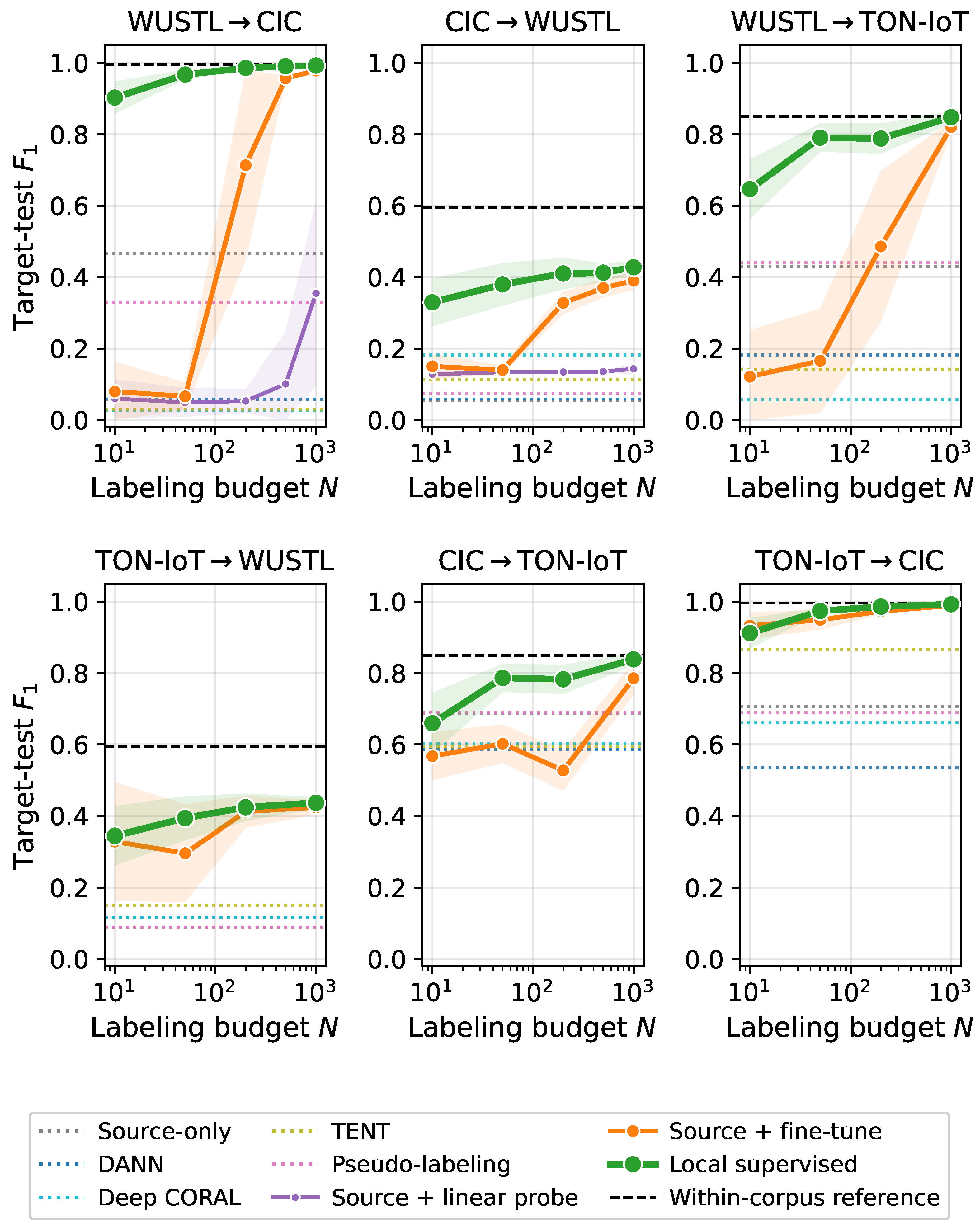
Figure 2. Target-test F 1 versus labeling budget N across all six cross-corpus directions, every cell aggregating 5 seeds × 3 replicates ( n = 15 ). Dotted horizontal lines are the five zero-target-label adaptation methods (source-only, DANN, Deep CORAL, TENT, pseudo-labeling); solid curves use N target labels (standard-deviation bands), with direct local-supervised training drawn as the heavy green curve; dashed black is the within-corpus reference of each target corpus. The local-supervised model matches or exceeds every transfer alternative and approaches the within-corpus ceiling in every direction. The linear probe appears in the primary-pair panels only.
Electronics 15 03015 g002
Statistical protocol. Unless a caption states otherwise, every reported cell aggregates 5 seeds × 3 few-shot replicates ( n = 15 runs, varying both the data split/model initialization and the drawn label set). Paired comparisons use Wilcoxon signed-rank tests with Holm–Bonferroni correction over 14 comparisons and bootstrap 95 % confidence intervals ( n boot = 2000 ). To guard against an unfair comparison favoring the local model, a hyperparameter-fairness ablation re-runs source-pretrain+fine-tune with the local-supervised optimization schedule, so that any residual gap cannot be attributed to a tuning mismatch.

6. Measuring Cross-Corpus Shift

We characterize the gap between corpora with three measurements. First, a Random Forest trained to predict “which corpus did this row come from” on the harmonized nine-feature schema reaches 100 % accuracy on every pair. Equivalently, the H-divergence proxy [12], defined as 2 ( 1 2 ϵ dom ) for domain-classifier error rate ϵ dom , saturates at 2.0 on every pair. Second, a quadratic-time kernel MMD [13] computed between 1500-row subsamples of source and target standardized features ranges over [ 0.70 , 0.98 ] across the primary sensor-network pairs ( 0.83 for WUSTL ↔ CIC, 0.98 for WUSTL ↔ TON-IoT, and 0.70 for CIC ↔ TON-IoT; the theoretical ceiling on the unit ball is 2 1.41 ), and the per-direction divergence for the complete four-corpus matrix is reported with the twelve-direction results in Section 7.4. We report the square-rooted unbiased kernel MMD estimate using an RBF kernel with median-heuristic bandwidth. Combined with the qualitative differences in attacks, threat models, and capture tools, these measurements place the evaluation in the severe-shift regime on every pair, and—through the H-divergence bound [12]—predict that marginal-alignment adaptation has little headroom.

6.1. Theoretical Interpretation via the Target-Error Bound

The measured divergence has a direct consequence in domain-adaptation theory. The bound of Ben-David et al. [12] states that for any hypothesis h the target risk obeys
ϵ T ( h ) ϵ S ( h ) + 1 2 d H Δ H ( D S , D T ) + λ ,
where λ = min h ϵ S ( h ) + ϵ T ( h ) is the error of the best joint hypothesis and d H Δ H is the symmetric-difference divergence. Treating the measured domain-classifier separability as an empirical proxy for the divergence term, the proxy saturates at 2.0 on every genuinely cross-corpus direction; the divergence contribution alone is therefore approximately 1 2 ( 2.0 ) = 1.0 , so Equation (1) reads ϵ T ( h ) ϵ S ( h ) + 1 + λ and is vacuous for practical target-risk prediction: it already exceeds the trivial error ceiling of 1.0 . Unlabeled methods that align marginals (DANN, Deep CORAL, TENT) minimize ϵ S and attempt to shrink the divergence term, but when the two corpora are near-perfectly separable in the harmonized space that term offers little purchase, and the conditional shift in attack semantics is absorbed into λ , which marginal alignment alone cannot be relied on to reduce. This is exactly the regime our empirical collapse occupies. Direct local-supervised training sidesteps Equation (1) altogether: by minimizing an empirical estimate of ϵ T on a small target-labeled sample it optimizes the quantity that the transfer bound can only loosely cap. This explains why, under the measured severe shift, a small target-labeled sample can outperform unlabeled source alignment.

6.2. Feature-Information Loss Versus Domain Shift

Mapping four native schemas onto a common nine-feature space discards information, so a fair reading of the transfer collapse must separate two distinct effects: the accuracy lost by compressing the feature space (feature-information loss) and the accuracy lost by moving between corpora (domain shift). We isolate the first effect by measuring within-corpus F 1 on the same corpus at three schema resolutions, holding the model and protocol fixed (Table 5). On WUSTL, the corpus that loses the most features, within-corpus F 1 falls from 0.655 on the full 30-feature native schema to 0.616 when the eight biometric columns are removed (22 flow-only features) and to 0.606 on the harmonized nine-feature schema. The harmonization step proper (from 22 flow features to 9) costs about one F 1 point; the larger part of the 5 -point total comes from dropping the biometric columns, not from harmonization. On the other corpora, the harmonized within-corpus references stay high ( F 1 = 0.996 for CIC, 0.98 for CSE-IDS2018, 0.85 for TON-IoT), so the nine-feature interface is not the bottleneck.
The two effects differ by an order of magnitude. Feature compression costs at most about five F 1 points within a corpus, whereas moving to a different corpus on the same nine-feature schema costs 40 to 90 points (CIC → WUSTL source-only reaches F 1 = 0.04 ). The transfer collapse is therefore a property of the shift between corpora, not an artifact of the harmonized representation; a richer per-corpus schema could recover a few points of within-corpus accuracy but would not close the cross-corpus gap, and it would also break the cross-corpus comparability that the audit requires. This is why the audit bounds, rather than measures, the best achievable transfer.

7. Results

7.1. Main Result Across Six Directions

Table 3 reports the six-direction headline at N = 50 : the strongest unlabeled DA baseline against source-pretrain+fine-tune (matched schedule) and direct local-supervised training, every cell aggregating the same 5 × 3 protocol ( n = 15 ). The grid uses stratified target-label draws so that source-pretrained and local-only methods consume exactly the same labeled examples; the deployed agent instead uses the k-medoids policy evaluated separately in Section 7.8. WUSTL ↔ CIC remains the primary IoMT case study. On WUSTL → CIC some unlabeled runs retain partial utility because CIC’s attacks carry strong volumetric signatures, but the source-only baseline is itself unstable in this direction: across the 15 runs its F 1 is trimodal—six runs at ≤0.04, three near 0.43 , and six near 0.93 (mean 0.47 )—so small-seed subsets of the identical protocol can produce means anywhere between 0.04 and 0.93 . This run-to-run instability is part of the negative result: a deployment cannot rely on a transfer baseline whose outcome depends on the training draw. On CIC → WUSTL every unlabeled method collapses (best mean F 1 = 0.18 , Deep CORAL). At N = 50 target labels, paired Wilcoxon tests with Holm–Bonferroni correction ( n = 15 ) yield p Holm 0.003 for direct local-supervised training versus each unlabeled baseline, with 15 / 15 wins per pair on both WUSTL ↔ CIC directions and bootstrap 95 % confidence intervals on Δ F 1 that exclude zero everywhere. Once the fine-tune schedule is matched, source pretraining is statistically indistinguishable from from-scratch local training: | Δ F 1 | 0.05 in all 24 ( N , direction ) cells of the fairness ablation across all six directions ( n = 15 each), so the practical advantage goes to the simpler local-only procedure.
Four mechanisms jointly explain the WUSTL-target collapse. First, the harmonized feature space exhibits both marginal shift (MMD = 0.83 for WUSTL ↔ CIC) and conditional shift: WUSTL attack flows are short-duration, high-jitter telemetry tampering, whereas CIC/TON-IoT attack flows are dominated by volumetric DDoS, scanning, and protocol abuse. Marginal-feature alignment cannot recover the target conditional, which is precisely the Zhao et al. [14] lower bound. Second, attack semantics differ across corpora: source classifiers learn volumetric-attack signatures that are absent from WUSTL’s medical-device-tampering label space, so the source decision boundary lies in a region of low target attack support. Third, the harmonized schema discards corpus-specific information (MQTT payloads, biometric telemetry) that the source model relied on; what remains under-determines the target label. Fourth, ρ X Y ( source ) and ρ X Y ( target ) disagree on the sign for several harmonized features (rate, jitter), so feature-only alignment moves the source representation away from the target’s class structure.
Statistical detail on the unlabeled-DA collapse appears in Table 4: Holm-corrected paired Wilcoxon tests ( n = 15 ) yield p Holm 0.003 in every cell, and direct local-supervised training wins 15 / 15 paired runs against every cross-corpus baseline on both WUSTL ↔ CIC directions. Bootstrap 95 % confidence intervals on Δ F 1 exclude zero everywhere. Table 4 focuses on the primary WUSTL ↔ CIC smart-health pair, where the formal protocol covers all eight methods; the TON-IoT directions are summarized at the same protocol in Table 3 and follow the same ordering. Table 4 reports as-published hyperparameter schedules; the matched-schedule comparison for source fine-tuning (Source+FT-matched) was reported above.

7.2. Agent Behavior Under Different Human-Labeling Budgets

Figure 1 plots target-test F 1 versus labeling budget N for all eight methods on the primary WUSTL ↔ CIC pair under the formal 5 × 3 protocol; the corresponding curves for all six directions appear in Figure 2. Five zero-target-label methods (dotted) do not depend on N; three N-target-label methods (solid, with standard-deviation bands) do. The agent’s local-supervised curve is approximately monotone in N on every direction. On WUSTL → CIC it reaches the within-corpus reference (dashed) by N 200 ( F 1 = 0.986 versus 0.996 ); on the hardest direction, CIC → WUSTL, it rises from 0.33 at N = 10 to a plateau of 0.43 at N = 1000 —about 70 % of the 0.60 within-corpus reference, with 0.38 of it already reached at N = 50 . The pattern justifies the 10–50 label budget that the agent procedure targets: most of the F 1 achievable from small local batches is captured at small budgets, and the marginal value of additional labels falls off quickly, which is the property that makes the human-in-the-loop step affordable.
Figure 2 extends these primary-pair budget curves to all six cross-corpus directions, with every cell at the same formal 5-seed × 3-replicate protocol as the main results ( n = 15 ). On the TON-IoT directions, the unlabeled baselines are budget-free horizontal references, the labeled curves cover N { 10 , 50 , 200 , 1000 } , and the linear probe is reported for the primary pair only. The qualitative ordering (unlabeled adaptation flat or collapsed, labeled methods monotone in N, local-supervised training matching matched fine-tuning) is the same in every panel.

7.3. Three-Corpus Cross-Transfer

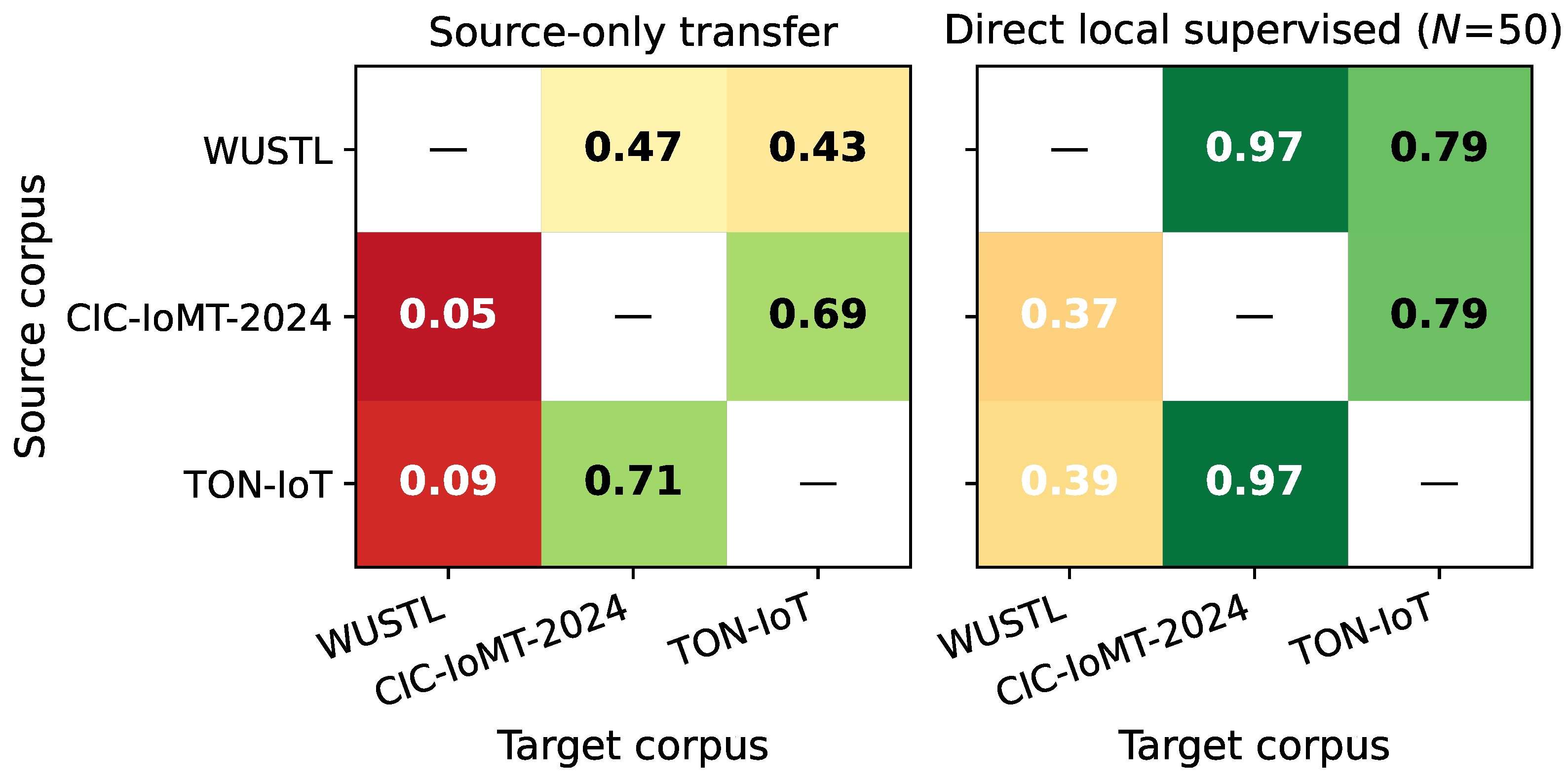
Adding TON-IoT [10] and re-running across all six pairwise directions on the same schema shows the pattern is not specific to WUSTL ↔ CIC (Figure 3). Shift is essentially maximal in every pair (H-divergence proxy = 2.0 , MMD [ 0.70 , 0.98 ] ). Source-only collapses on both WUSTL-target directions (below F 1 = 0.15 from both CIC and TON-IoT; per-direction values in Table 6) and is erratic elsewhere; direct local-supervised training reaches F 1 0.37 in every cell at N = 50 (mean 0.71 versus a source-only mean of 0.41 ). Source+fine-tune (matched) ties local-supervised training cell-by-cell to within | Δ F 1 | 0.05 , replicating the WUSTL ↔ CIC fairness pattern across six directions.

7.4. The Full Four-Corpus Transfer Matrix

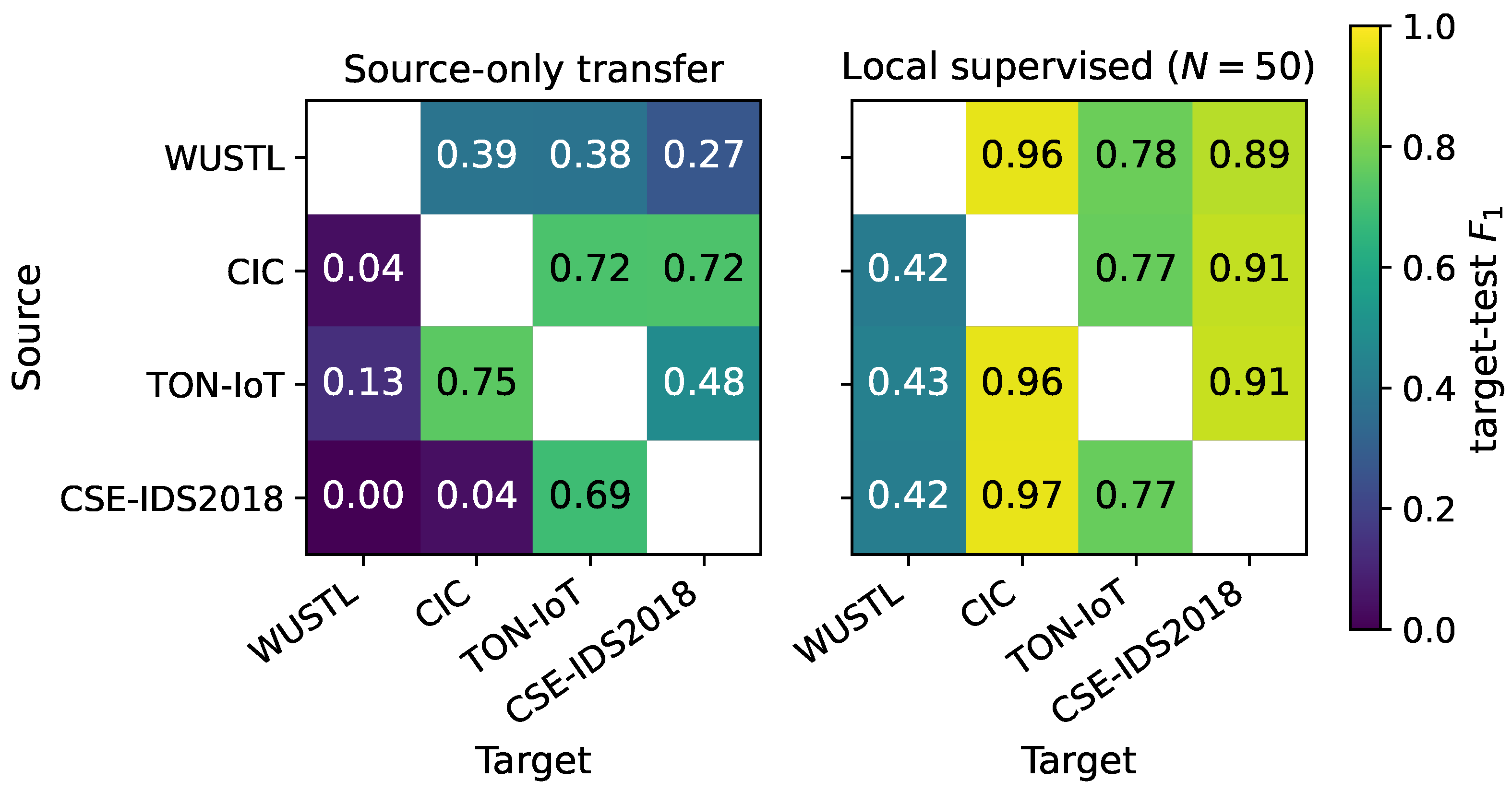
Section 7.1, Section 7.2 and Section 7.3 worked through the sensor-network corpora; the complete picture spans all four corpora and their twelve ordered transfer directions (Table 6, Figure 4). Each cell trains on one corpus and tests on another at N = 50 over five seeds, and the primary WUSTL ↔ CIC and six-direction analyses additionally carry the three few-shot replicates of the formal protocol. CSE-IDS2018, drawn from an unrelated enterprise capture, anchors the non-medical corner of the matrix.
Every direction sits at the maximal H-divergence ( 2.0 , two at 1.99 ): the four corpora are mutually and near-perfectly separable in the harmonized space. The pattern established on the sensor-network pairs carries straight through. Averaged over the twelve directions, source-only transfer reaches F 1 = 0.38 and falls apart on the hardest targets ( 0.00 on CSE-IDS2018 → WUSTL, 0.04 on CIC → WUSTL and CSE-IDS2018 → CIC, 0.13 on TON-IoT → WUSTL), while direct local-supervised training holds F 1 0.41 in every cell (mean 0.77 , max 0.97 ). The enterprise corpus behaves like the medical ones: as a target it admits source-only transfer at only 0.49 on average against 0.91 for local supervision. Source-pretrain+fine-tune under the matched schedule tracks local-only training to within | Δ F 1 | 0.03 in all twelve directions, so from-scratch local training is the operational choice across the entire matrix, medical and non-medical alike. Numbers may differ slightly from the six-direction figures because Table 6 uses five seeds without the three few-shot replicates of the primary protocol.

7.5. Source-Free Adaptation (SHOT)

The unlabeled baselines examined so far span adversarial, moment-matching, test-time, and self-training adaptation; SHOT [26] is the dedicated source-free member of the same suite. Introduced with the method set in Section 5, it freezes the source-trained classifier and adapts the feature encoder on target-unlabeled data by information maximization and centroid pseudo-labeling. Because SHOT uses no target labels, it is directly comparable to the other zero-target-label baselines; we evaluate it across all twelve directions at the five-seed protocol (Table 7).
The outcome matches the rest of the audit. SHOT improves on the source-only baseline in some directions (for example CSE-IDS2018 → CIC, 0.04 0.55 ) but degrades it in others (TON-IoT → CIC, 0.75 0.49 ; WUSTL → CIC, 0.39 0.24 ), because information maximization on the target marginal can settle on a confidently mislabeled cluster structure under severe shift. On the three medical-telemetry (WUSTL) targets it collapses to F 1 0.13 , the same failure mode as the other unlabeled methods. Averaged over the twelve directions SHOT reaches F 1 = 0.43 , against 0.38 for source-only and 0.77 for direct local-supervised training, and it stays below local-supervised training in every one of the twelve directions. A recent source-free method therefore does not escape the conditional-shift ceiling of Section 6.1: it adjusts the target marginal but cannot recover the target label-conditional, so the small local-labeled sample remains the better choice.

7.6. Operational Precision–Recall Tradeoffs

F 1 summarizes but hides the precision/recall tradeoffs that determine whether the agent is deployable. The alarming unlabeled cross-corpus methods on CIC → WUSTL (Deep CORAL, DANN, TENT) fire on 66– 99 % of benign flows in exchange for catching 39– 82 % of attacks; direct local-supervised training reaches a false-positive rate (FPR) = 0.19 at recall = 0.59 on CIC → WUSTL and FPR = 0.02 at recall = 0.94 on WUSTL → CIC. Source-only is the only unlabeled baseline that keeps FPR low ( 0.001 ), but its recall of 0.02 is near-silent. Concretely, on a single CIC → WUSTL split at N = 50 : source-only flags 16 of 614 attacks; Source+FT-default flags 342 at the cost of 3847 false alarms; direct local-supervised training flags 434 at 1241 false alarms. For an operations center, the difference between a near-silent detector and one that surfaces most attacks at a manageable false-alarm load is the difference between an unusable and a usable deployment.

7.7. Edge-Deployment Footprint

The agent fits within an IoT-gateway resource envelope (Table 1): a 1206-parameter model at 4.7 KB float32, training from 50 labels in under one second on a single CPU thread, and inference at 0.6 ms per 1000 flows. The slowest unlabeled baseline (pseudo-label) takes 16 s, still tractable on the gateway but unnecessary given that direct local-supervised training matches it. The footprint indicates that the workflow can run on commodity gateway-class CPU hardware without requiring a GPU.

7.8. Active Labeling and Representative-Flow Selection

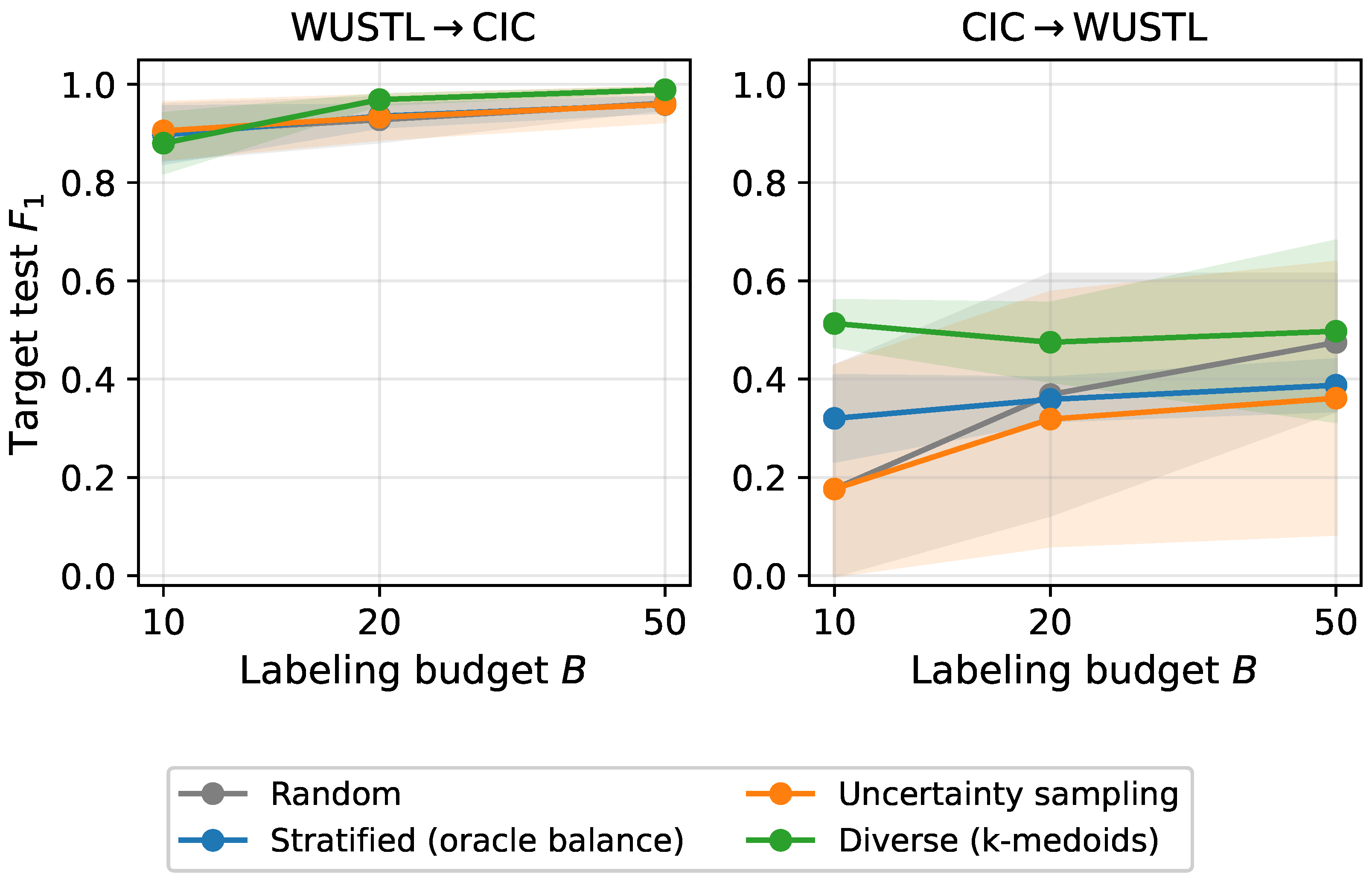
Because the agent depends on limited human feedback, its sample-selection policy is central to deployment performance. The main-grid comparisons of Section 7.1 use stratified draws to isolate the transfer question; this section isolates the selection question. The agent uses k-medoids [29] as its representative-flow selection policy over standardized nine-feature vectors: medoids minimize within-cluster dissimilarity and therefore cover the local target distribution more efficiently than random sampling. Figure 5 compares four selectors over 15 seeds: random, stratified ( 50 / 50 oracle balance), uncertainty sampling [30,31] (lowest model confidence), and diverse (k-medoids). On CIC → WUSTL at B = 10 , diverse selection reaches F 1 = 0.51 ± 0.05 versus random 0.18 ± 0.25 ( 2.91 × the mean, with much smaller variance); diverse leads at B = 20 and ties random at B = 50 . Notably, the k-medoids policy at B = 10 already exceeds the level that stratified draws reach at N = 50 in Table 3 on this hardest direction ( 0.51 versus 0.37 ), which is why the deployed agent uses k-medoids rather than the analysis-oriented stratified draw. On WUSTL → CIC all four selectors lie within 3 percentage points at B = 10 because CIC’s volumetric attacks are distinctive. The variance reduction is operationally as important as the mean improvement: a selection policy that removes the chance of a near-useless labeling round is easier to trust in deployment.

7.9. Robustness to Analyst Label Noise

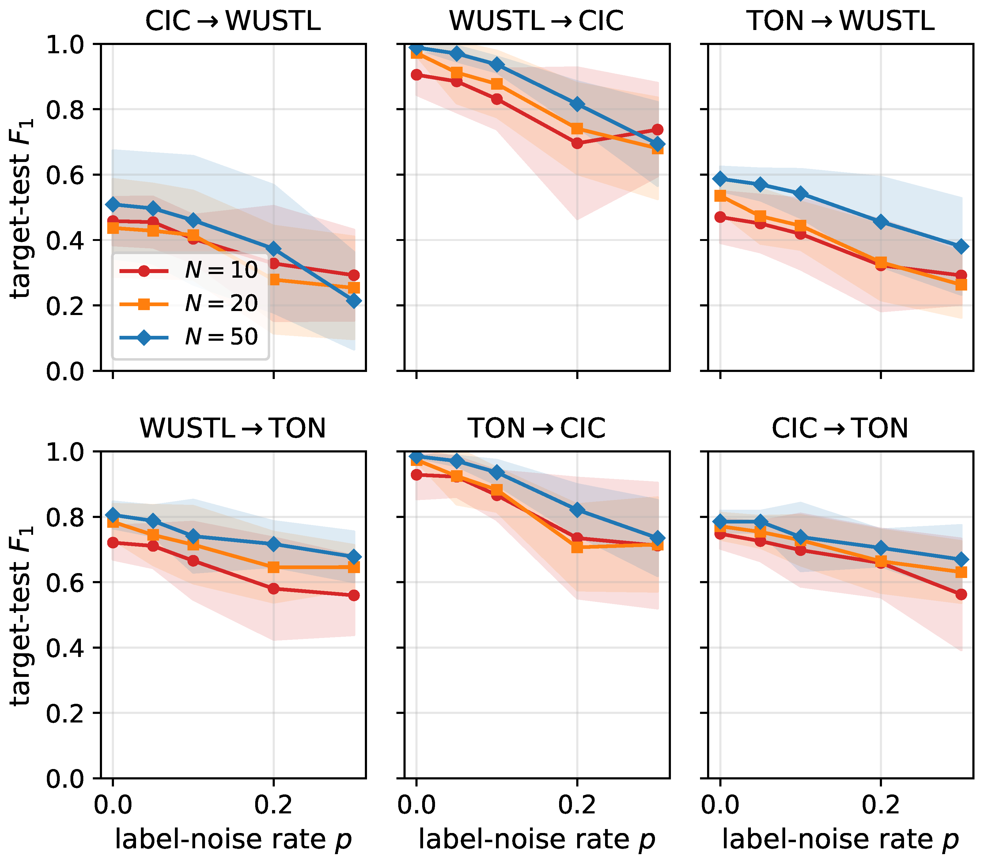
The agent assumes that the analyst labels the selected medoid flows correctly, but real analysts make mistakes. We quantify the sensitivity of the local-supervised step to imperfect labels with symmetric label noise: after the agent selects its N medoid flows, each oracle label is flipped independently with probability p { 0 , 0.05 , 0.10 , 0.20 , 0.30 } before the model is trained, and the trained model is evaluated on the clean target-test set. Each cell uses n = 15 runs (5 seeds × 3 replicates that vary both the medoid-selection seed and the noise realization), with the same architecture, optimization schedule, and quantile scaling as the main experiments.
Figure 6 shows the resulting degradation across all six directions. The decline is gradual, with no abrupt collapse at any tested rate. At N = 50 , averaged over the six directions, mean F 1 falls from 0.78 (clean labels) to 0.76 at p = 0.05 and 0.73 at p = 0.10 , a cost of 1.4 and 5.1 percentage points, respectively, while heavier noise costs materially more ( 0.65 at p = 0.20 and 0.56 at p = 0.30 ). The hardest direction is also the most sensitive: on CIC → WUSTL at N = 50 , F 1 drops from 0.51 clean to 0.46 at p = 0.10 and 0.21 at p = 0.30 , whereas the easy volumetric-attack directions (e.g., WUSTL → CIC: 0.99 0.94 at p = 0.10 ) absorb moderate noise with little loss. Smaller budgets amplify the effect, since a single flipped label is 10 % of an N = 10 batch. In operational terms, the human-in-the-loop procedure tolerates the error rates expected of an attentive analyst (roughly up to 10 % ) at a cost of at most a few F 1 points, but it does not survive careless labeling: label quality on the small medoid batch matters more than adding further labels, consistent with the budget-curve saturation in Section 7.2.

7.10. Architecture and Feature Ablations

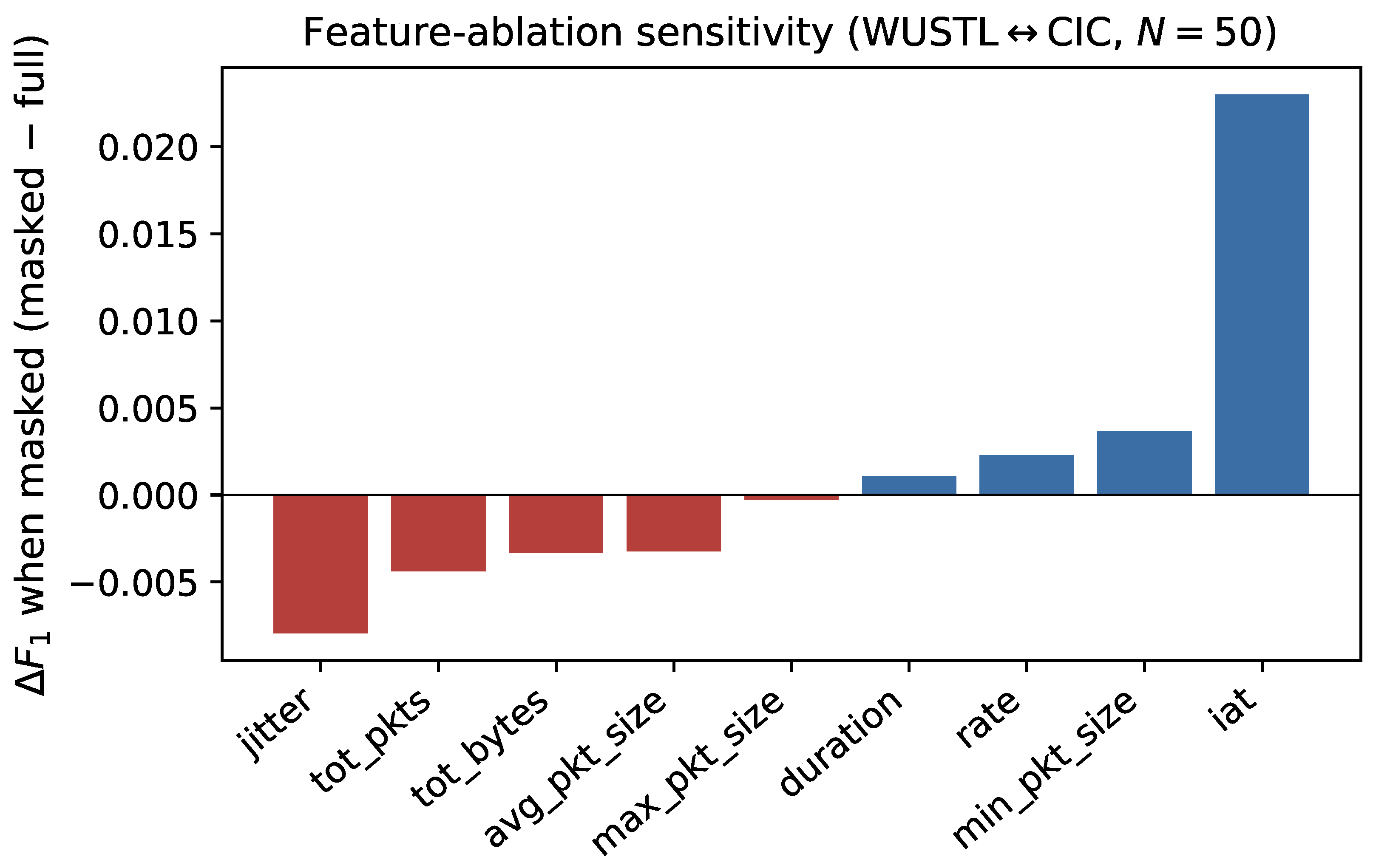
Two ablations justify the model and feature choices behind the 1206-parameter network, both in the local-supervised regime at N = 50 . First, we compare five from-scratch model families on the six original directions, five seeds each (Table 8). The tiny MLP is not a compromise for the sake of size: it attains the highest mean target-test F 1 ( 0.719 ) and the best mean on the hardest WUSTL-target directions ( 0.420 ), edging out a three-fold larger MLP (3926 parameters; 0.714 ), a 200-tree Random Forest ( 0.705 ), a depth-8 decision tree ( 0.685 ), and logistic regression ( 0.675 ). Capacity beyond a thousand parameters buys nothing here because the binding constraint is the fifty target labels, not model expressivity—which is precisely why an edge-sized model is the right tool rather than a concession. Second, masking each harmonized feature in turn (setting it to its standardized mean and retraining) leaves target-test F 1 on the primary WUSTL ↔ CIC pair almost unchanged: most features shift it by less than 0.01 (Figure 7), so no single feature dominates the decision rule and the nine-feature schema degrades gracefully under feature loss—a desirable property for a gateway that may transiently lose a telemetry field. Inter-arrival time is the only feature whose removal materially moves the metric, and it slightly improves mean F 1 ( + 0.023 ), indicating it carries more cross-corpus noise than signal in the harmonized space.

7.11. Adversarial Robustness

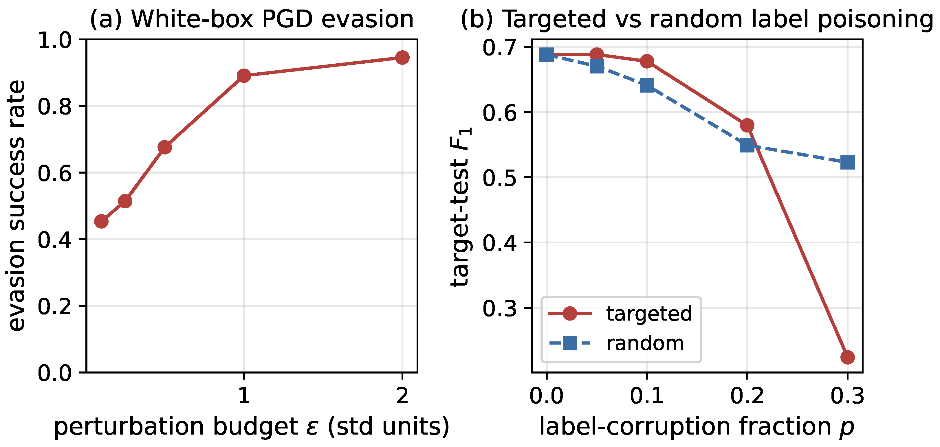
The symmetric-noise study bounds non-adversarial analyst error; two worst-case security threats complete the robustness picture for the deployed local-supervised model. (a) Evasion. A white-box L projected-gradient attack [32,33] in the agent’s standardized feature space, applied to malicious target-test flows the detector classifies correctly, flips 45 % of them to benign at a budget of 0.1 standard deviations and 95 % at 2.0 (Figure 8a). Like every lightweight ML detector, the tiny model offers a limited robustness margin; we report this as a deployer-relevant bound rather than a robustness claim, and note that gradient-based evasion presumes white-box access that a gateway-resident model does not freely grant. (b) Targeted label poisoning. Modeling a compromised or deceived analyst [34] who flips a fraction p of the malicious labels in the 50-flow batch to benign—the attack-suppressing direction—target-test F 1 falls from 0.69 to 0.22 at p = 0.30 , versus 0.52 under symmetric random flipping at the same rate (Figure 8b). The two regimes cross over: at low corruption ( p 0.10 ) targeted suppression is gentler than random flipping because it removes only a few of the 25 malicious labels, but beyond p = 0.20 it concentrates damage on the attack class and collapses recall. The asymmetry sharpens the operational message: label integrity on the malicious class matters more than label quantity, so protecting the analyst-labeling channel is a first-order security requirement, not a hygiene afterthought.

8. Drift-Aware Human-in-the-Loop Agent Workflow

The empirical results translate into a concrete drift-aware agent loop (Figure 9 and Algorithm 1), an instance of the detect-then-retrain pattern from the concept-drift literature [27,28] placed at the IoMT gateway. The agent collects a recent-traffic sample ( 10 K rows), clusters the standardized features with k-medoids at K { 10 , , 50 } so that each medoid is a representative flow, and asks the IT analyst to label those medoids. In deployment, the analyst would label each selected medoid from its flow metadata, alert context, device identity, and available local logs; the public-corpus experiments approximate this step with oracle labels, and Section 7.9 bounds the cost of analyst error through controlled noise injection. At 30 s per flow, 10 labels take roughly five minutes and 50 labels roughly 25 min; at 60 s per flow, the same budgets take ten and fifty minutes. The agent then trains the 1206-parameter MLP from scratch on those labels ( < 1 s on CPU; Table 3 reports the stratified analysis-grid result and Section 7.8 the deployed k-medoids selection result at N = 50 ), deploys the local IDS on the on-premises gateway (Table 1), and monitors drift on incoming traffic via a moving-window MMD on the harmonized features, retraining weekly or monthly or whenever drift exceeds a calibrated threshold. The procedure needs no cross-institutional data sharing; because labels and telemetry stay on-premises, it reduces the need to export medical-device telemetry to third parties and thereby lowers privacy and governance exposure under regimes such as HIPAA and GDPR Article 9.

8.1. Closed-Loop Validation of the Drift Trigger

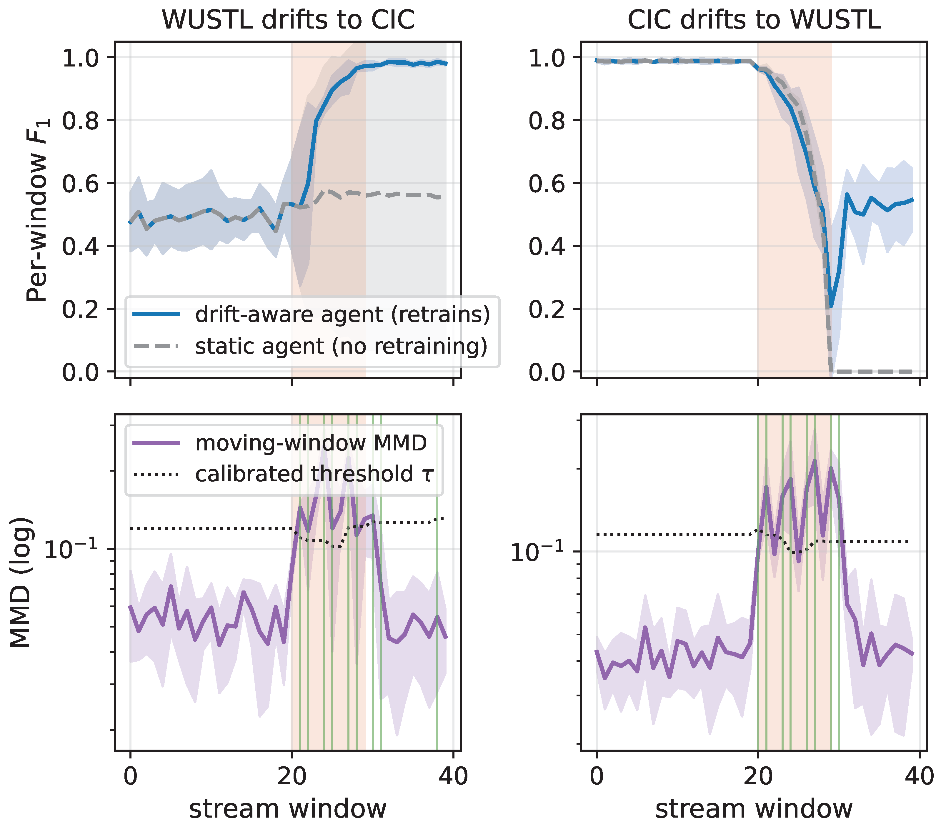
The loop in Algorithm 1 is only useful if the MMD trigger actually fires when the traffic distribution moves and stays quiet when it does not. We validate the loop end-to-end on simulated gateway streams with injected drift. Each stream consists of 40 windows of 500 flows; window t is an i.i.d. draw from the mixture ( 1 α t ) A + α t B of two corpora on the harmonized schema, with α t = 0 for the first 20 windows and then either an abrupt jump to 1 or a linear ramp over 10 windows. Cross-corpus substitution is the same severe-shift proxy used throughout the paper, so these streams represent a worst-case distribution change. The agent is deployed exactly as in Algorithm 1: it bootstraps from K = 50 medoid labels on initial traffic, computes a moving-window MMD (fixed median-heuristic bandwidth) between each incoming window and the training-time reference, and retrains from scratch on 50 fresh medoid labels whenever the statistic exceeds τ , where τ is the q-quantile of a null distribution obtained from disjoint random splits of the reference window. A static agent (identical initial model, no retraining) runs on the same stream as the comparison. We use 5 seeds per configuration and sweep q { 0.90 , 0.95 , 0.99 , 0.999 } .
Figure 10 shows the gradual-drift traces at the q = 0.99 operating point, and Table 9 reports the threshold sweep. Three observations summarize the outcome. First, detection is fast and specific: at q = 0.99 , the trigger fires within at most two windows of drift onset (at most 1000 flows) on every gradual stream and immediately on every abrupt stream, with zero false triggers across the 200 stationary gradual windows and 3 across the 200 stationary abrupt windows ( 0.75 % of the 400 stationary windows overall). Second, retraining restores the local reference level: on CIC-drifts-to-WUSTL, where the static agent collapses to F 1 = 0.00 , the monitored agent recovers to 0.53 ( 0.51 abrupt), the within-corpus level achievable from 50 medoid labels on WUSTL (Section 7.8), and on WUSTL-drifts-to-CIC it reaches 0.98 versus 0.38 0.56 for the static agent. Third, the threshold controls a sensible tradeoff: lowering q to 0.90 gains at most one window of earlier detection but doubles the false-trigger count, and each unnecessary trigger costs one 50-label analyst round; q = 0.99 balances the two. Gradual drift naturally produces 4 retrains as the mixture keeps moving away from each new reference (roughly one labeling round per ramp stage, about 25 analyst-minutes each at 30 s per flow), while abrupt drift settles after 1–2.

8.2. Justification of the MMD Drift Trigger

The trigger uses a moving-window MMD; Table 10 asks whether that choice is justified against four standard concept-drift detectors on identical WUSTL ↔ CIC streams (gradual and abrupt profiles, five seeds), all observing the same non-adapting deployed model so that the comparison isolates detector quality. The two distribution-based detectors that watch the covariate stream directly—the MMD trigger and a per-feature Kolmogorov–Smirnov test, both null-calibrated at q = 0.99 —detect drift within half a window on average, with zero false alarms in the stationary prefix and 100 % detection. The error-based detectors are uniformly worse: DDM [35] fires constantly on the fluctuating per-flow error signal (32 false alarms per stream), while Page–Hinkley [36] and ADWIN [37] are slower ( 1.6 and 3.5 windows) and miss 20– 30 % of drift episodes, because a rise in label-error must accumulate before it is visible, and at test time the labels needed to compute that error are exactly what the gateway lacks. Watching the input distribution rather than the unavailable error is therefore the right signal for an unsupervised retraining trigger; MMD matches the simpler KS statistic on this binary task while extending naturally to the full multivariate feature vector and to higher-order shift that per-feature tests miss.

9. Discussion

The contribution is a deployment audit of a constrained edge AI agent showing that modest human feedback can outperform or match cross-corpus adaptation under severe shift. Practically, the results favor labeling a small representative sample of recent local traffic and training the compact model on-premises, rather than deploying a public-corpus IDS as-is or adding an adaptation pipeline whose matched-schedule benefit is negligible. The near-saturated single-corpus F 1 values reported throughout the IoMT IDS literature should be read as within-corpus references, not as predictions of cross-environment performance. The negative transfer result follows from conditional shift between corpora that differ in attack semantics and capture methodology, the regime in which marginal-alignment adaptation is fundamentally limited.

9.1. Validity and Scope of the Cross-Corpus Proxy

The audit uses cross-corpus shift as a stand-in for cross-hospital deployment shift, and the two are not identical. Public corpora differ in collection environment, attack taxonomy, and feature-construction toolchain, while two hospitals running similar equipment may differ far less. The most likely direction of the mismatch is that the cross-corpus proxy over-states the shift a typical hospital pair would see, because different capture pipelines and attack catalogs are more dissimilar than two deployments of the same clinical technology. Read that way, the proxy is a conservative, near-worst-case setting for the transfer question. Where local labeling already matches or beats transfer under maximal separability, it should remain competitive under the milder shift of two similar hospitals. Where a target instead resembles an available public corpus closely, transfer may do better, and the drift monitor is what flags the in-between case. The proxy is therefore informative about the deployment decision (label locally versus import and adapt) rather than a numerical predictor of any specific hospital’s F 1 . Its applicable scope is the common situation in which the target environment is not known in advance to match a public corpus; it does not cover the case where a vendor has a corpus drawn from the same device population as the target, which would warrant a direct transfer test.
The simulated drift streams inherit this proxy character. Cross-corpus substitution is a strong, fast distribution change, whereas real IoMT drift is usually slower and subtler: firmware and device-population turnover, shifting clinical workflows, and gradually evolving attacks rather than a wholesale corpus swap. The reported detection delays are therefore a best case for signal strength. What does carry over is the threshold calibration, which is distribution-free (the trigger fires on a null quantile estimated from the reference window itself), so the false-alarm control transfers even though sensitivity to gentler drift is not established here. Stressing the trigger on subtler profiles is left to future work.

9.2. Scalability to Larger and Heterogeneous IoMT Deployments

The workflow scales by replication rather than by growing a single model. Each gateway trains and monitors its own 1206-parameter detector on its own traffic, so a larger or more heterogeneous deployment adds independent per-gateway instances rather than a centralized model that must fit every device population at once. The per-gateway cost is fixed and small: a K [ 10 , 50 ] analyst-labeling round (about 5 to 25 min), sub-second CPU training, and a moving-window MMD computed on fixed-size windows and subsamples, so its per-window cost is bounded regardless of the total traffic volume. Heterogeneity is handled locally: each instance learns the distribution of the subnet it sits on, and the drift monitor triggers a fresh local round when that subnet changes. This avoids asking one model to generalize across heterogeneous subnets, which is precisely the cross-environment transfer that this paper shows is unreliable. The main coordination cost of scale is human: more gateways mean more occasional labeling rounds, which the calibrated trigger is designed to keep infrequent. Sharing labeling effort across similar gateways, and federating the local models without exporting raw telemetry, are natural extensions for very large estates and are noted in future work.

9.3. Limitations

Six limitations bound the claims. (i) Cross-corpus shift between public datasets is a reproducible proxy for cross-hospital deployment, not a substitute; no public corpus pairs two captures from two distinct hospitals, so the hospital-to-hospital shift magnitude is unmeasured. Section 9.1 discusses the validity and scope of this proxy and the related drift realism. (ii) The harmonized nine-feature schema discards dataset-specific information; richer per-corpus features may close part of the gap, and the audit therefore bounds rather than measures the best achievable transfer. (iii) The adversarial analysis (Section 7.11) covers white-box evasion and targeted label-suppression on the deployed model, but we do not model a fully adaptive adversary that co-evolves with the agent across repeated retraining rounds, nor a black-box query-limited attacker. (iv) Analyst labels may be noisy in real deployments; Section 7.9 bounds the cost of symmetric noise (about five F 1 points at a 10 % error rate with N = 50 ) and Section 7.11 quantifies the worst case of attack-label suppression, but other structured mislabeling patterns (an analyst systematically deceived about a particular attack family) remain unmeasured. (v) Public IDS datasets differ from live hospital telemetry in device populations, capture pipelines, and operational drift profiles, so absolute F 1 values are within-corpus references rather than direct estimates of production performance. (vi) The study targets binary attack/benign detection. Real hospital deployments ultimately need finer-grained attack categorization and response-oriented actions (isolating a device, escalating an alert, applying a playbook), which a binary detector does not provide on its own. We scope the detector as the first-stage gateway triage layer that decides whether a flow warrants attention, feeding a second-stage classifier or analyst workflow for attribution and response. Binary scope also avoids the invalid multiclass label mappings that arise across corpora with incompatible attack taxonomies, which is what makes the cross-corpus audit well defined. Extending the local-supervised step to multi-class attack-family attribution, where the same harmonized features and labeling budget would have to support more classes, is future work.

10. Future Work

The limitations point to concrete extensions. The most direct is an evaluation on paired captures from two real hospital IoMT subnets, which would replace the cross-corpus proxy with a measured hospital-to-hospital shift and the public-corpus oracle labels with real analyst labels; this is the validation step needed before operational claims, and the on-premises design is intended to make such a study feasible without exporting telemetry. A related extension scales the workflow across many gateways by sharing labeling effort between similar subnets and federating the local models without exporting raw flows, and adds multi-class attack-family attribution on top of the binary triage layer. A second direction extends the adversarial analysis of Section 7.11 (which already quantifies white-box evasion and targeted label-suppression) to a fully adaptive adversary that co-evolves with the agent across retraining rounds and to black-box, query-limited evasion against the gateway-resident model, including poisoning concentrated on the informative medoids the agent selects. A third is to stress the drift trigger of Section 8.1 on subtler profiles than cross-corpus substitution (seasonal load changes, device-population turnover, and slow sensor-firmware drift on real long-running traffic), where the drift signal-to-noise ratio is lower, and to couple the calibrated threshold with retraining-cost-aware policies that weigh each 50-label analyst round against the expected accuracy recovery.

11. Conclusions

We presented a drift-aware human-in-the-loop edge AI agent for IoMT intrusion detection and audited its deployment behavior under cross-corpus shift as a reproducible proxy for cross-hospital deployment. Across all four corpora, spanning medical IoMT (WUSTL-EHMS-2020, CIC-IoMT-2024), general IoT/IIoT (TON-IoT), and enterprise traffic (CSE-CIC-IDS-2018), the harmonized feature distributions are highly distinguishable, and the negative-transfer pattern is the same in the medical and non-medical directions alike. Over all twelve transfer directions, unlabeled adaptation is unstable and source pretraining provides no measurable advantage over from-scratch training once the fine-tuning schedule is matched; a domain-adaptation error bound, driven vacuous by the measured separability, anticipates this behavior. The agent automates traffic summarization, representative-flow selection, lightweight local training, inference, and drift monitoring while preserving human control over labeling. The tiny 1206-parameter model is supported by architecture and feature ablations: larger or classical alternatives do not materially improve the deployment tradeoff, and no single harmonized feature dominates the decision rule. Robustness tests also delimit the approach: the local model absorbs realistic (≤10%) symmetric analyst error at a cost of a few F 1 points, but targeted malicious-to-benign label suppression and white-box feature-space evasion remain meaningful threats, so protecting the labeling channel and the model internals is an operational requirement. Finally, the closed-loop evaluation and detector comparison show the calibrated MMD trigger gives fast, low-false-alarm retraining decisions under severe simulated drift, where error-based detectors lag or miss. Under the evaluated severe cross-corpus shift, the evidence favors labeling a small representative sample of recent local traffic and training a compact model on-premises, rather than deploying a public-corpus IDS as-is or relying on marginal-alignment adaptation.


Funding

This research was funded by the Ongoing Research Funding program, grant number ORF-2026-1464, King Saud University, Riyadh, Saudi Arabia.

Institutional Review Board Statement

This study used only publicly available, de-identified network-traffic intrusion-detection corpora and did not involve human subjects or identifiable patient data; institutional review board approval was therefore not required.

Informed Consent Statement

Not applicable.

Data Availability Statement

The four datasets used in this study are publicly available from their original providers: WUSTL-EHMS-2020 [7], CIC-IoMT-2024 [8], TON-IoT [10], and CSE-CIC-IDS-2018 [11]. The preprocessing scripts, feature mappings, fixed seeds, per-seed result files, and the scripts for the ablation, adversarial, and drift-detector experiments are available from the author upon reasonable request.

Acknowledgments

Generative AI tools were used solely for language and formatting refinement; the author reviewed and approved all content and takes full responsibility for the work.

Conflicts of Interest

The author declares no conflicts of interest. The funder had no role in the design of the study; in the collection, analyses, or interpretation of data; in the writing of the manuscript; or in the decision to publish the results.

References

  1. Ghubaish, A.; Salman, T.; Zolanvari, M.; Unal, D.; Al-Ali, A.; Jain, R. Recent Advances in the Internet-of-Medical-Things (IoMT) Systems Security. IEEE Internet Things J. 2021, 8, 8707–8718. [Google Scholar] [CrossRef] [Scilit]
  2. Newaz, A.I.; Sikder, A.K.; Rahman, M.A.; Uluagac, A.S. A Survey on Security and Privacy Issues in Modern Healthcare Systems: Attacks and Defenses. ACM Trans. Comput. Healthc. 2021, 2, 27. [Google Scholar] [CrossRef] [Scilit]
  3. Putra, K.T.; Arrayyan, A.Z.; Hayati, N.; Firdaus; Damarjati, C.; Bakar, A.; Chen, H.C. A Review on the Application of Internet of Medical Things in Wearable Personal Health Monitoring: A Cloud-Edge Artificial Intelligence Approach. IEEE Access 2024, 12, 21437–21452. [Google Scholar] [CrossRef] [Scilit]
  4. Han, S.; Mao, H.; Dally, W.J. Deep Compression: Compressing Deep Neural Networks with Pruning, Trained Quantization and Huffman Coding. In Proceedings of the International Conference on Learning Representations (ICLR), San Juan, Puerto Rico, 2–4 May 2016. [Google Scholar]
  5. Kang, Y.; Hauswald, J.; Gao, C.; Rovinski, A.; Mudge, T.; Mars, J.; Tang, L. Neurosurgeon: Collaborative Intelligence Between the Cloud and Mobile Edge. In Proceedings of the 22nd International Conference on Architectural Support for Programming Languages and Operating Systems (ASPLOS), Xi’an, China, 8–12 April 2017; pp. 615–629. [Google Scholar] [CrossRef] [Scilit]
  6. Eskandari, M.; Janjua, Z.H.; Vecchio, M.; Antonelli, F. Passban IDS: An Intelligent Anomaly-Based Intrusion Detection System for IoT Edge Devices. IEEE Internet Things J. 2020, 7, 6882–6897. [Google Scholar] [CrossRef] [Scilit]
  7. Hady, A.A.; Ghubaish, A.; Salman, T.; Unal, D.; Jain, R. Intrusion Detection System for Healthcare Systems Using Medical and Network Data: A Comparison Study. IEEE Access 2020, 8, 106576–106584. [Google Scholar] [CrossRef] [Scilit]
  8. Dadkhah, S.; Pinto Neto, E.C.; Ferreira, R.; Molokwu, R.C.; Sadeghi, S.; Ghorbani, A.A. CICIoMT2024: A Benchmark Dataset for Multi-Protocol Security Assessment in IoMT. Internet Things 2024, 28, 101351. [Google Scholar] [CrossRef] [Scilit]
  9. Tahsien, S.M.; Karimipour, H.; Spachos, P. Machine Learning Based Solutions for Security of Internet of Things (IoT): A Survey. J. Netw. Comput. Appl. 2020, 161, 102630. [Google Scholar] [CrossRef] [Scilit]
  10. Alsaedi, A.; Moustafa, N.; Tari, Z.; Mahmood, A.; Anwar, A. TON_IoT Telemetry Dataset: A New Generation Dataset of IoT and IIoT for Data-Driven Intrusion Detection Systems. IEEE Access 2020, 8, 165130–165150. [Google Scholar] [CrossRef] [Scilit]
  11. Sharafaldin, I.; Lashkari, A.H.; Ghorbani, A.A. Toward Generating a New Intrusion Detection Dataset and Intrusion Traffic Characterization. In Proceedings of the 4th International Conference on Information Systems Security and Privacy (ICISSP), Funchal, Portugal, 22–24 January 2018; pp. 108–116. [Google Scholar]
  12. Ben-David, S.; Blitzer, J.; Crammer, K.; Kulesza, A.; Pereira, F.; Vaughan, J.W. A Theory of Learning from Different Domains. Mach. Learn. 2010, 79, 151–175. [Google Scholar] [CrossRef] [Scilit]
  13. Gretton, A.; Borgwardt, K.M.; Rasch, M.J.; Schölkopf, B.; Smola, A. A Kernel Two-Sample Test. J. Mach. Learn. Res. 2012, 13, 723–773. [Google Scholar]
  14. Zhao, H.; Combes, R.T.d.; Zhang, K.; Gordon, G. On Learning Invariant Representations for Domain Adaptation. In Proceedings of the International Conference on Machine Learning (ICML), Long Beach, CA, USA, 9–15 June 2019. [Google Scholar]
  15. Sommer, R.; Paxson, V. Outside the Closed World: On Using Machine Learning for Network Intrusion Detection. In Proceedings of the IEEE Symposium on Security and Privacy (S&P), Oakland, CA, USA, 16–19 May 2010; pp. 305–316. [Google Scholar] [CrossRef] [Scilit]
  16. Arp, D.; Quiring, E.; Pendlebury, F.; Warnecke, A.; Pierazzi, F.; Wressnegger, C.; Cavallaro, L.; Rieck, K. Dos and Don’ts of Machine Learning in Computer Security. In Proceedings of the 31st USENIX Security Symposium (USENIX Security), Boston, MA, USA, 10–12 August 2022; pp. 3971–3988. [Google Scholar]
  17. Engelen, G.; Rimmer, V.; Joosen, W. Troubleshooting an Intrusion Detection Dataset: The CICIDS2017 Case Study. In Proceedings of the IEEE Security and Privacy Workshops (SPW), Virtual, 27 May 2021; pp. 7–12. [Google Scholar] [CrossRef] [Scilit]
  18. Layeghy, S.; Portmann, M. Explainable Cross-Domain Evaluation of ML-Based Network Intrusion Detection Systems. Comput. Electr. Eng. 2023, 108, 108692. [Google Scholar] [CrossRef] [Scilit]
  19. Apruzzese, G.; Pajola, L.; Conti, M. SoK: The Impact of Unlabelled Data in Cyberthreat Detection. In Proceedings of the IEEE European Symposium on Security and Privacy (EuroS&P), Genoa, Italy, 6–10 June 2022. [Google Scholar]
  20. Ganin, Y.; Lempitsky, V. Unsupervised Domain Adaptation by Backpropagation. In Proceedings of the International Conference on Machine Learning (ICML), Lille, France, 7–9 July 2015. [Google Scholar]
  21. Sun, B.; Saenko, K. Deep CORAL: Correlation Alignment for Deep Domain Adaptation. In Proceedings of the European Conference on Computer Vision Workshop on Transferring and Adapting Source Knowledge in Computer Vision (TASK-CV), Amsterdam, The Netherlands, 11–14 October 2016. [Google Scholar] [CrossRef] [Scilit]
  22. Wang, D.; Shelhamer, E.; Liu, S.; Olshausen, B.; Darrell, T. TENT: Fully Test-Time Adaptation by Entropy Minimization. In Proceedings of the International Conference on Learning Representations (ICLR), Virtual, 3–7 May 2021. [Google Scholar]
  23. Saenko, K.; Kulis, B.; Fritz, M.; Darrell, T. Adapting Visual Category Models to New Domains. In Proceedings of the European Conference on Computer Vision (ECCV), Crete, Greece, 5–11 September 2010. [Google Scholar] [CrossRef] [Scilit]
  24. Long, M.; Cao, Y.; Wang, J.; Jordan, M.I. Learning Transferable Features with Deep Adaptation Networks. In Proceedings of the International Conference on Machine Learning (ICML), Lille, France, 7–9 July 2015. [Google Scholar]
  25. Quiñonero-Candela, J.; Sugiyama, M.; Schwaighofer, A.; Lawrence, N.D. (Eds.) Dataset Shift in Machine Learning; MIT Press: Cambridge, MA, USA, 2009. [Google Scholar]
  26. Liang, J.; Hu, D.; Feng, J. Do We Really Need to Access the Source Data? Source Hypothesis Transfer for Unsupervised Domain Adaptation. In Proceedings of the International Conference on Machine Learning (ICML), Virtual, 13–18 July 2020; pp. 6028–6039. [Google Scholar]
  27. Gama, J.; Žliobaitė, I.; Bifet, A.; Pechenizkiy, M.; Bouchachia, A. A Survey on Concept Drift Adaptation. ACM Comput. Surv. 2014, 46, 44. [Google Scholar] [CrossRef] [Scilit] [PubMed]
  28. Lu, J.; Liu, A.; Dong, F.; Gu, F.; Gama, J.; Zhang, G. Learning under Concept Drift: A Review. IEEE Trans. Knowl. Data Eng. 2019, 31, 2346–2363. [Google Scholar] [CrossRef] [Scilit]
  29. Kaufman, L.; Rousseeuw, P.J. Finding Groups in Data: An Introduction to Cluster Analysis; John Wiley & Sons: Hoboken, NJ, USA, 1990. [Google Scholar]
  30. Lewis, D.D.; Gale, W.A. A Sequential Algorithm for Training Text Classifiers. In Proceedings of the 17th Annual International ACM SIGIR Conference on Research and Development in Information Retrieval (SIGIR), Dublin, Ireland, 3–6 July 1994; pp. 3–12. [Google Scholar]
  31. Settles, B. Active Learning Literature Survey; Technical Report 1648; Department of Computer Sciences, University of Wisconsin–Madison: Madison, WI, USA, 2009. [Google Scholar]
  32. Goodfellow, I.J.; Shlens, J.; Szegedy, C. Explaining and Harnessing Adversarial Examples. In Proceedings of the International Conference on Learning Representations (ICLR), San Diego, CA, USA, 7–9 May 2015. [Google Scholar]
  33. Madry, A.; Makelov, A.; Schmidt, L.; Tsipras, D.; Vladu, A. Towards Deep Learning Models Resistant to Adversarial Attacks. In Proceedings of the International Conference on Learning Representations (ICLR), Vancouver, BC, Canada, 30 April–3 May 2018. [Google Scholar]
  34. Biggio, B.; Nelson, B.; Laskov, P. Poisoning Attacks against Support Vector Machines. In Proceedings of the 29th International Conference on Machine Learning (ICML), Edinburgh, UK, 26 June–1 July 2012; pp. 1807–1814. [Google Scholar]
  35. Gama, J.; Medas, P.; Castillo, G.; Rodrigues, P. Learning with Drift Detection. In Proceedings of the Advances in Artificial Intelligence (SBIA 2004); Lecture Notes in Computer Science; Springer: Berlin/Heidelberg, Germany, 2004; Volume 3171, pp. 286–295. [Google Scholar]
  36. Page, E.S. Continuous Inspection Schemes. Biometrika 1954, 41, 100–115. [Google Scholar] [CrossRef] [Scilit]
  37. Bifet, A.; Gavaldà, R. Learning from Time-Changing Data with Adaptive Windowing. In Proceedings of the 2007 SIAM International Conference on Data Mining (SDM), Minneapolis, MN, USA, 26–28 April 2007; pp. 443–448. [Google Scholar]
Figure 3. Cross-corpus F 1 across three public IDS corpora at N = 50 , mean over 5 seeds × 3 replicates per cell. Left: source-only transfer collapses on hard targets. Right: direct local-supervised training recovers operational F 1 on every off-diagonal cell. Color encodes F 1 (darker is lower).
Electronics 15 03015 g003
Figure 4. Twelve-direction transfer over the four corpora at N = 50 (mean of five seeds); CSE-IDS2018 is the non-medical enterprise corpus. Left: source-only transfer collapses on hard targets (dark cells). Right: direct local-supervised training recovers operational F 1 in every off-diagonal cell.
Electronics 15 03015 g004
Figure 5. Active labeling strategies for the agent, 15 seeds with standard-deviation bands. k-medoids at B = 10 reaches F 1 = 0.51 ± 0.05 on CIC → WUSTL ( 2.91 × the mean of random selection).
Electronics 15 03015 g005
Figure 6. Robustness of the agent’s local-supervised training to symmetric analyst label noise at rate p, across all six cross-corpus directions and labeling budgets N { 10 , 20 , 50 } . Mean target-test F 1 over n = 15 runs with standard-deviation bands. Degradation is graceful up to p = 0.10 and substantial beyond p = 0.20 , with the hardest direction (CIC → WUSTL) the most sensitive.
Electronics 15 03015 g006
Figure 7. Feature-ablation sensitivity on WUSTL↔CIC at N = 50 (mean over five seeds): change in target-test F 1 (masked − full) when each harmonized feature is masked. Most effects are small, indicating that no single feature dominates the decision rule. Negative bars mark features whose removal slightly degrades F 1 ; the single positive bar (inter-arrival time) marks a feature whose removal slightly improves it, suggesting direction-specific noise rather than dependence on that feature. Bar color shows the sign of the effect (negative or positive).
Electronics 15 03015 g007
Figure 8. Adversarial robustness of the local-supervised agent. (a) White-box L PGD evasion success rises with the perturbation budget. (b) Targeted label poisoning (malicious → benign suppression) is far more damaging than symmetric random flipping beyond p = 0.2 , collapsing target-test F 1 . Evasion is averaged over the six cross-corpus directions and poisoning over the primary WUSTL ↔ CIC pair, five seeds each.
Electronics 15 03015 g008
Figure 9. Drift-aware human-in-the-loop IDS agent workflow. The edge agent observes recent local traffic, selects representative medoid flows for analyst labeling, trains a tiny local MLP, performs on-premises inference, monitors distribution drift, and triggers retraining while preserving human authority over labels.
Electronics 15 03015 g009
Figure 10. Closed-loop behavior of the drift-aware agent on simulated gateway streams with gradual cross-corpus drift (mean over 5 seeds, standard-deviation bands; q = 0.99 ). Top: per-window F 1 of the monitored agent versus the static (never-retrained) agent; the shaded span marks the drift ramp. Bottom: the moving-window MMD crosses the calibrated threshold τ (dotted) at drift onset; green lines mark retraining events. On CIC-drifts-to-WUSTL the static agent collapses to F 1 = 0.00 while the monitored agent recovers to the local 50-label reference level.
Electronics 15 03015 g010
Table 1. Edge-deployment footprint of the agent. Measurements on a single CPU thread (Intel x86_64, warm cache, no GPU); times averaged over five seeds.
PropertyValue
Architecture 9 32 16 2 MLP
Parameters1206
Model size (float32) 4.7  KB
Training, local-sup ( N = 50 ) < 1  s
Training, slowest baseline 16  s
Inference latency 0.6  ms/1K flows
Compute device1 CPU thread
Table 2. Semantic mapping from each corpus’s native schema onto the harmonized nine-feature schema. For TON-IoT, b s , b d , p s , p d denote src_bytes, dst_bytes, src_pkts, dst_pkts; packet-size minima/maxima and jitter have no native counterpart and degenerate to the average packet size and 0. CSE-IDS2018 uses CICFlowMeter fields (F/B abbreviate forward/backward).
HarmonizedWUSTL-EHMS-2020CIC-IoMT-2024TON-IoTCSE-IDS2018
rateRateRate ( p s + p d ) / duration Flow Pkts/s
durationDurDurationdurationFlow Duration
iatmean (SIntPkt, DIntPkt)IAT duration / ( p s + p d ) Flow IAT Mean
tot_bytesTotBytesTot sum b s + b d TotLen F+B
tot_pktsTotPktsNumber p s + p d Tot F+B Pkt
min_pkt_sizemin (sMinPktSz, dMinPktSz)Minavg. pkt. sizePkt Len Min
max_pkt_sizemax (sMaxPktSz, dMaxPktSz)Maxavg. pkt. sizePkt Len Max
avg_pkt_sizeTotBytes/TotPktsAVG ( b s + b d ) / ( p s + p d ) Avg Pkt Size
jittermean (SrcJitter, DstJitter)Std0Pkt Len Std
Table 3. Six-direction summary at N = 50 , mean target-test F 1 over 5 seeds × 3 replicates ( n = 15 per cell). Best unlabel. is the strongest of source-only, DANN, Deep CORAL, TENT, and pseudo-label per direction. FT-matched is source-pretrain plus fine-tune under the local-supervised schedule.
DirectionBest Unlabel.FT-MatchedLocal-Sup
CIC → WUSTL 0.18 (CORAL) 0.38 0.37
WUSTL → CIC 0.47 (src-only) 0.96 0.97
TON-IoT → WUSTL 0.15 (TENT) 0.40 0.39
WUSTL → TON-IoT 0.44 (pseudo) 0.77 0.79
CIC → TON-IoT 0.69 (pseudo) 0.78 0.79
TON-IoT → CIC 0.87 (TENT) 0.97 0.97
Table 4. Direct local-supervised vs. each cross-corpus baseline at N = 50 . Δ F 1 = per-run paired difference (local-sup − baseline) over n = 15 runs (5 seeds × 3 replicates); 95 % CI is bootstrap (2000 resamples). Local-sup wins 15 / 15 paired runs on every row; paired Wilcoxon–Holm-corrected over 14 comparisons yields p Holm 0.003 in every row.
DirectionBaseline Δ F 1 [95% CI]
CIC → WUSTLsource-only + 0.32  [0.29,0.36]
DANN + 0.32  [0.28,0.36]
Deep CORAL + 0.20  [0.16,0.25]
TENT + 0.27  [0.24,0.30]
pseudo-lab. + 0.31  [0.25,0.36]
Src+LP + 0.25  [0.22,0.28]
Src+FT-def + 0.24  [0.21,0.27]
WUSTL → CICsource-only + 0.50  [0.30,0.70]
DANN + 0.91  [0.85,0.96]
Deep CORAL + 0.94  [0.93,0.95]
TENT + 0.94  [0.92,0.95]
pseudo-lab. + 0.64  [0.40,0.82]
Src+LP + 0.92  [0.90,0.94]
Src+FT-def + 0.90  [0.88,0.92]
Table 5. Feature-information loss isolated from domain shift on WUSTL (within-corpus F 1 from a Random Forest probe under the same stratified 70 / 30 protocol, mean over five seeds; a model-agnostic probe is used because the input dimension differs across the three schemas). Compressing the schema costs at most 5   F 1 points, an order of magnitude less than the cross-corpus collapse, which reaches 40–90 points (e.g., CIC → WUSTL source-only F 1 = 0.04 for the deployed MLP). Feature loss therefore cannot account for the transfer failure.
Schema (Within-Corpus WUSTL)Features F 1
Native, full30 0.655
Native, flow-only (drop biometrics)22 0.616
Harmonized9 0.606
Cross-corpus CIC → WUSTL (source-only)9 0.038
Table 6. Twelve-direction transfer audit over the four corpora at N = 50 , mean over five seeds; CSE-IDS2018 is the non-medical enterprise corpus. This matrix is reported over five seeds, whereas the primary WUSTL ↔ CIC and six-direction analyses (Table 3 and Table 4) use the full 5 × 3 few-shot protocol. All twelve directions are at near-maximal H-divergence. Source-only collapses on hard targets while direct local-supervised training stays operational in every cell, and source+fine-tune (matched) tracks it to within | Δ F 1 | 0.03 . Bold marks the direct local-supervised model (the recommended deployment choice); it is the row maximum in every direction except TON-IoT → CIC, where source+fine-tune (matched) is higher by 0.01 .
SourceTargetMMDH-DivSrc-OnlyLocal-SupSrc+FT
WUSTLCIC 0.83 2.00 0.386 0.962 0.958
WUSTLTON-IoT 0.98 2.00 0.382 0.777 0.771
WUSTLCSE-IDS2018 0.87 2.00 0.271 0.893 0.873
CICWUSTL 0.83 2.00 0.038 0.418 0.406
CICTON-IoT 0.71 2.00 0.716 0.769 0.763
CICCSE-IDS2018 0.76 2.00 0.720 0.910 0.904
TON-IoTWUSTL 0.98 2.00 0.134 0.434 0.428
TON-IoTCIC 0.70 2.00 0.747 0.965 0.975
TON-IoTCSE-IDS2018 0.72 1.99 0.484 0.915 0.914
CSE-IDS2018WUSTL 0.87 2.00 0.000 0.424 0.406
CSE-IDS2018CIC 0.76 2.00 0.043 0.965 0.940
CSE-IDS2018TON-IoT 0.73 1.99 0.688 0.769 0.752
Mean over 12 directions 0.384 0.767 0.758
Table 7. SHOT (source-free domain adaptation) over the twelve directions, mean over five seeds; SHOT uses no target labels. SHOT is unstable across directions, collapses on the WUSTL medical-telemetry targets, and stays below direct local-supervised training ( N = 50 ) in every direction. Source-only and local-supervised values are from the same runs for reference. Bold marks the highest F 1 in each row.
SourceTargetSrc-OnlySHOTLocal-Sup
WUSTLCIC 0.389 0.238 0.962
WUSTLTON-IoT 0.382 0.459 0.777
WUSTLCSE-IDS2018 0.271 0.554 0.893
CICWUSTL 0.038 0.125 0.418
CICTON-IoT 0.716 0.514 0.769
CICCSE-IDS2018 0.720 0.762 0.910
TON-IoTWUSTL 0.134 0.076 0.434
TON-IoTCIC 0.747 0.486 0.965
TON-IoTCSE-IDS2018 0.484 0.660 0.915
CSE-IDS2018WUSTL 0.000 0.067 0.424
CSE-IDS2018CIC 0.043 0.550 0.965
CSE-IDS2018TON-IoT 0.688 0.628 0.769
Mean over 12 directions 0.384 0.427 0.767
Table 8. Architecture ablation: mean target-test F 1 at N = 50 over the six original cross-corpus directions (×five seeds), and the mean restricted to the hardest WUSTL-target directions. The 1206-parameter MLP used throughout the paper is the strongest model on both columns. Bold marks the adopted model and its best scores; a dash marks models with no well-defined parameter count.
ModelParameters F 1 (All 6 Dir.) F 1 (→WUSTL)
Logistic regression10 0.675 0.383
Decision tree (depth 8) 0.685 0.364
Random forest (200) 0.705 0.401
MLP-wide ( 64 32 )3926 0.714 0.409
MLP-tiny ( 32 16 ) 1206 0.719 0.420
Table 9. Threshold sweep for the drift trigger. τ is the q-quantile of the split-reference null MMD. Delay is windows from drift onset to first trigger (1 window = 500 flows); false triggers are counted over the 200 stationary windows per row (2 scenarios × 5 seeds × 20 windows); retrains and final F 1 (last 8 windows) are means over the 10 streams per row.
ProfileqDelay (Mean)Delay (Max)False Trig.Retrains F 1 Final (Agent) F 1 Final (Static)
gradual 0.90 0.7 16 4.6 0.75 0.28
gradual 0.95 0.8 12 4.2 0.77 0.28
gradual 0.99 1.0 20 4.0 0.75 0.28
gradual 0.999 1.0 20 3.9 0.75 0.28
abrupt 0.90 0.1 15 1.5 0.74 0.19
abrupt 0.95 0.1 15 1.5 0.74 0.19
abrupt 0.99 0.0 03 1.3 0.74 0.19
abrupt 0.999 0.0 02 1.2 0.74 0.19
Table 10. Drift-detector comparison on identical WUSTL ↔ CIC streams (gradual+abrupt, five seeds; n = 20 streams per detector), all observing the same non-adapting model. Delay is windows from drift onset to first post-onset trigger; false alarms are stationary-prefix triggers per stream; detection rate is the fraction of streams detected. Distribution-based detectors (MMD, KS) dominate the error-based ones. Bold marks the proposed MMD trigger.
DetectorMean Delay (Windows)False Alarms/StreamDetection Rate
MMD (ours) 0.45 0.0 1.00
KS (per-feature) 0.45 0.0 1.00
DDM 1.07 32.4 0.70
Page–Hinkley 1.57 0.0 0.70
ADWIN 3.50 0.0 0.80
Disclaimer/Publisher’s Note: The statements, opinions and data contained in all publications are solely those of the individual author(s) and contributor(s) and not of MDPI and/or the editor(s). MDPI and/or the editor(s) disclaim responsibility for any injury to people or property resulting from any ideas, methods, instructions or products referred to in the content.