Author Contributions
Conceptualization, J.S., G.W. and F.Z.; methodology, J.S., G.W. and F.Z.; software, J.S. and F.Z.; validation, J.S.; investigation, F.Z.; visualization, J.S.; project administration, J.S.; supervision, G.W. and F.Z.; writing—original draft preparation, J.S.; writing—review and editing, F.Z. All authors have read and agreed to the published version of the manuscript.
Figure 1.
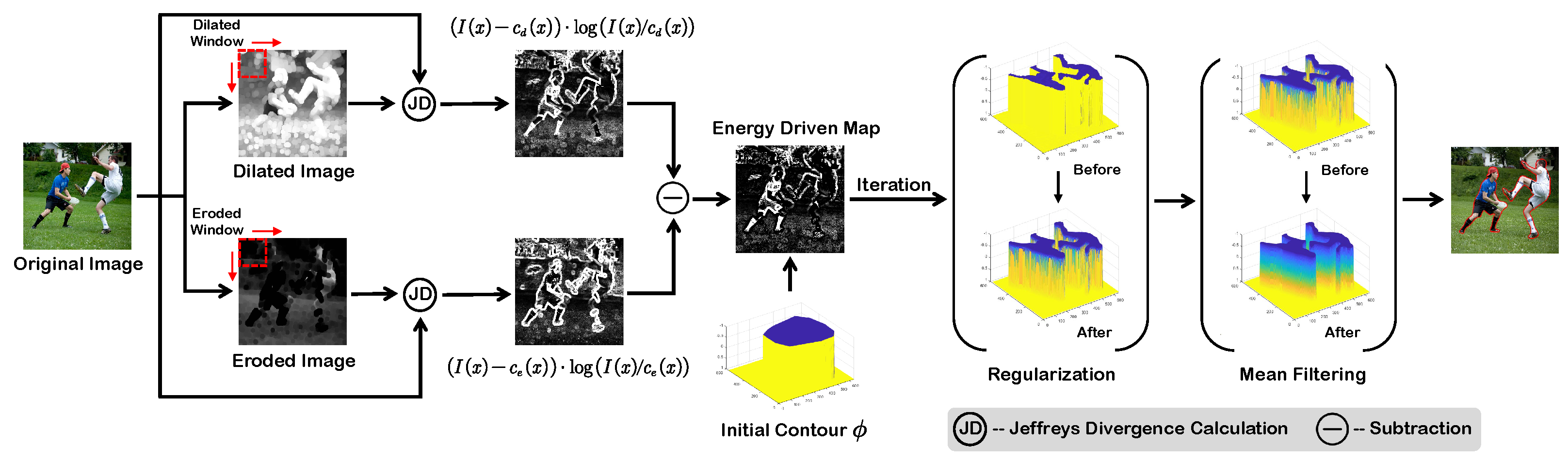
Overall pipeline of the MFJD-Seg framework. Structuring elements are leveraged to apply morphological erosion and dilation, which capture fundamental features. The red arrow indicates the direction of motion of the sliding window. By computing Jeffreys divergence between the original image and its eroded and dilated counterparts, enhanced feature maps are derived. The integration of these two maps yields the final energy-driven map, which provides the iterative driving force for the contour. To ensure numerical stability, we employ regularization to smooth the level set and improve parameter robustness, complemented by mean filtering to eliminate redundant noise components.
Figure 1.
Overall pipeline of the MFJD-Seg framework. Structuring elements are leveraged to apply morphological erosion and dilation, which capture fundamental features. The red arrow indicates the direction of motion of the sliding window. By computing Jeffreys divergence between the original image and its eroded and dilated counterparts, enhanced feature maps are derived. The integration of these two maps yields the final energy-driven map, which provides the iterative driving force for the contour. To ensure numerical stability, we employ regularization to smooth the level set and improve parameter robustness, complemented by mean filtering to eliminate redundant noise components.
Figure 2.
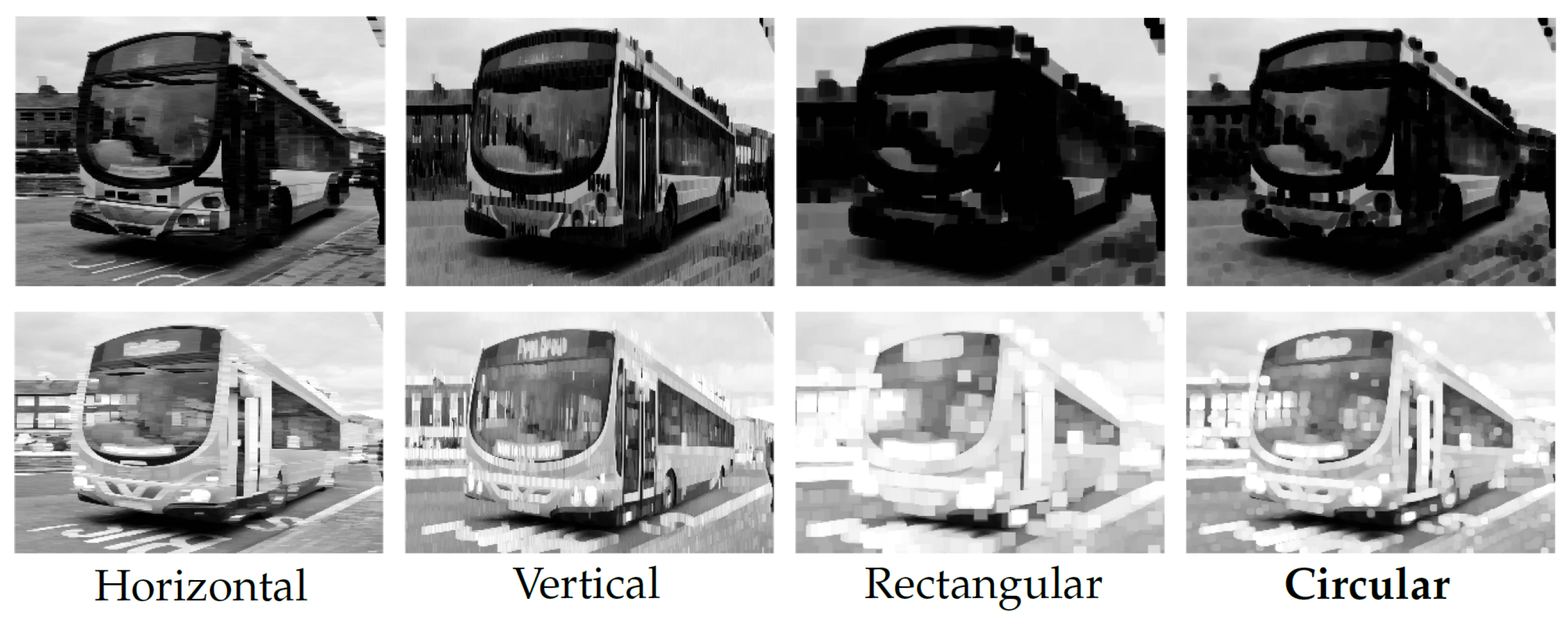
Visualization of different structuring element geometries. Row 1: eroded images. Row 2: dilated images.
Figure 2.
Visualization of different structuring element geometries. Row 1: eroded images. Row 2: dilated images.
Figure 3.
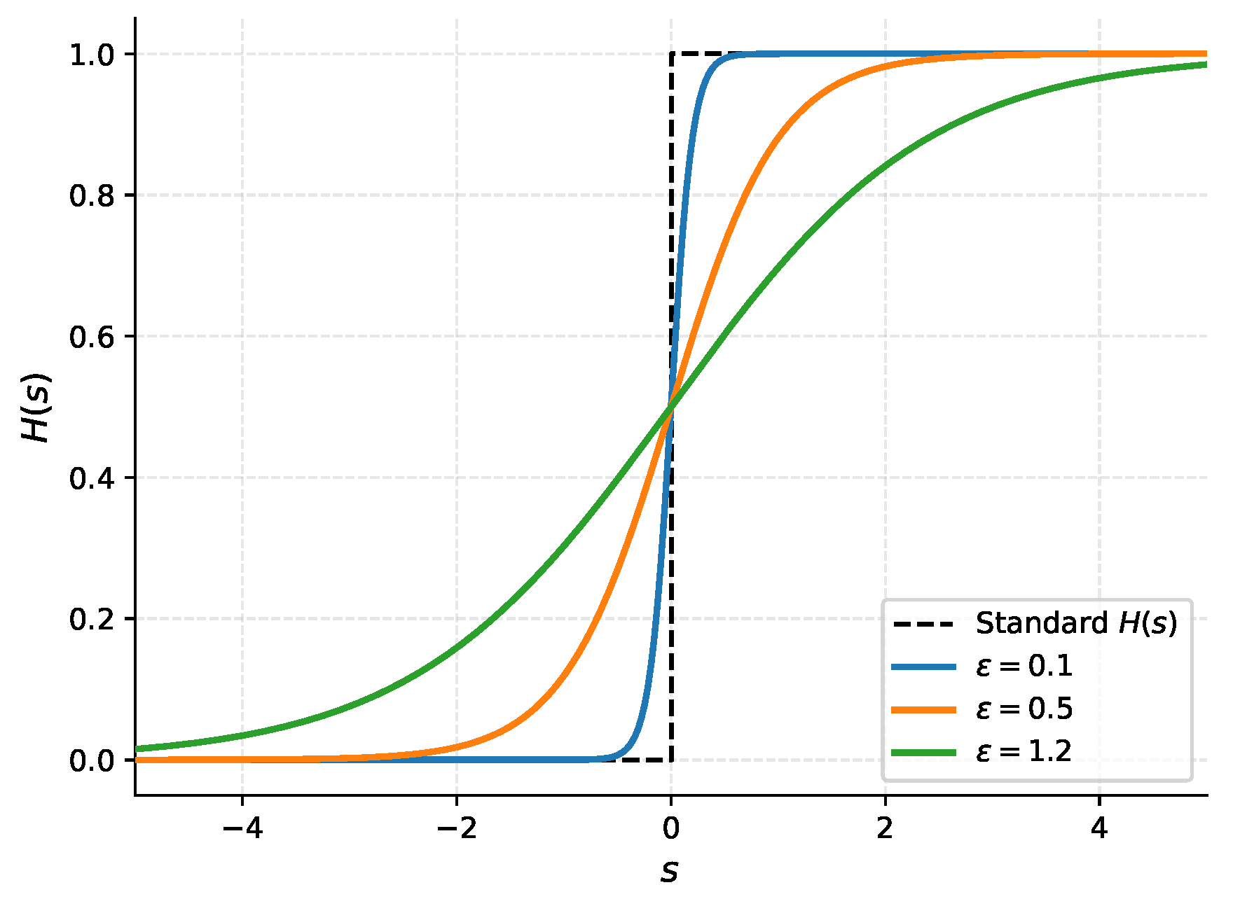
Comparison of the standard Heaviside function and our smoothed approximation.
Figure 3.
Comparison of the standard Heaviside function and our smoothed approximation.
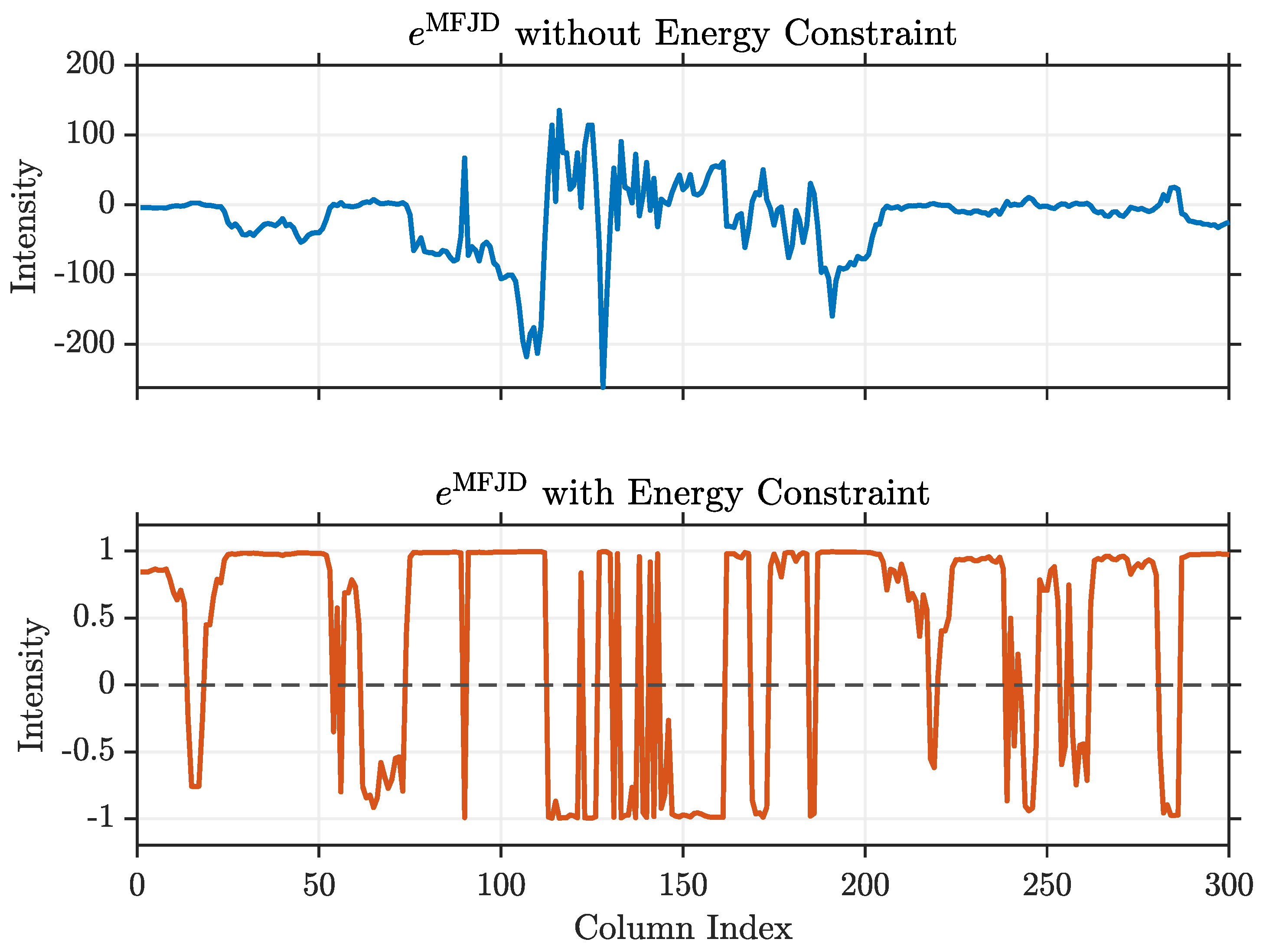
Figure 4.
Comparison of curves with and without the energy constraint.
Figure 4.
Comparison of curves with and without the energy constraint.
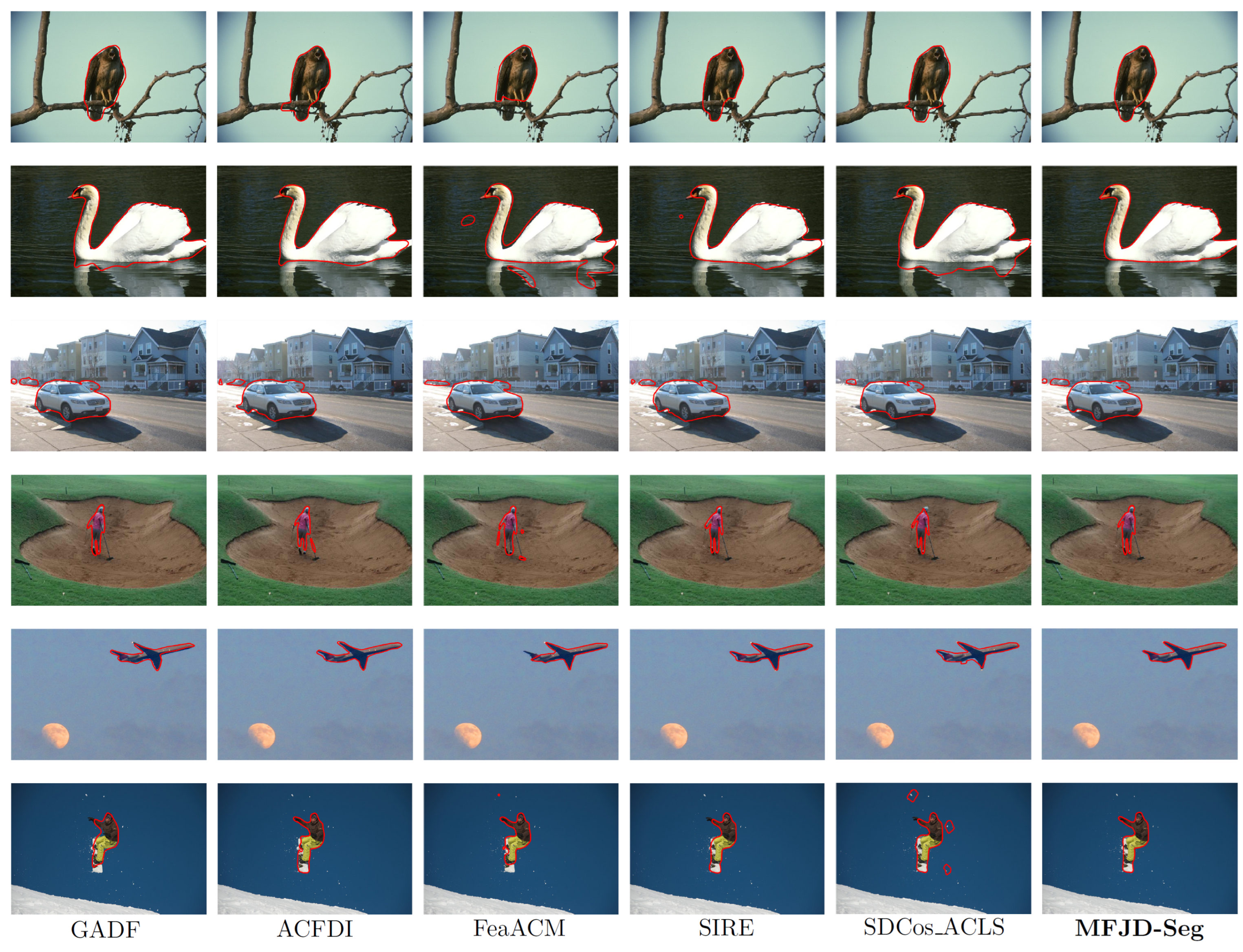
Figure 5.
Visualization of segmentation results for different ACMs.
Figure 5.
Visualization of segmentation results for different ACMs.
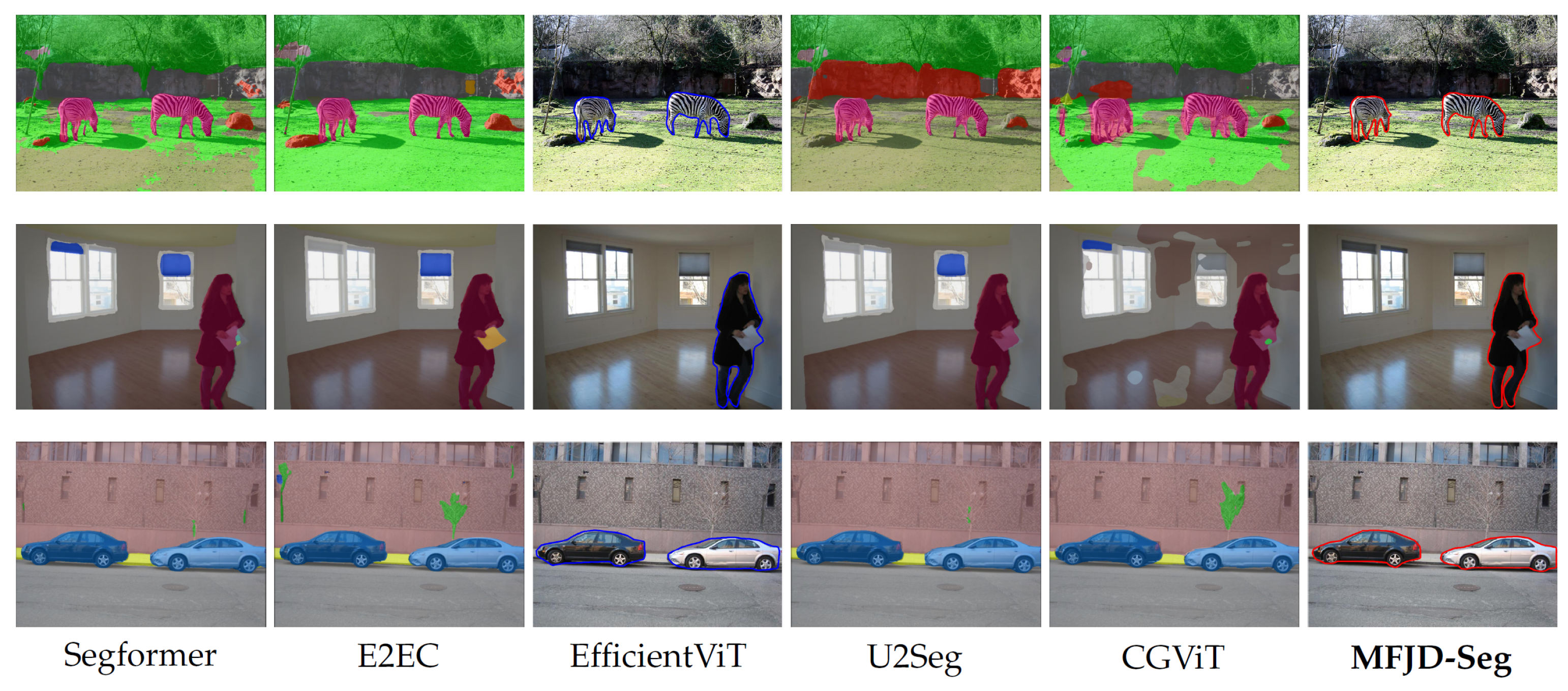
Figure 6.
Visualization of segmentation results for different deep learning models and MFJD-Seg.
Figure 6.
Visualization of segmentation results for different deep learning models and MFJD-Seg.
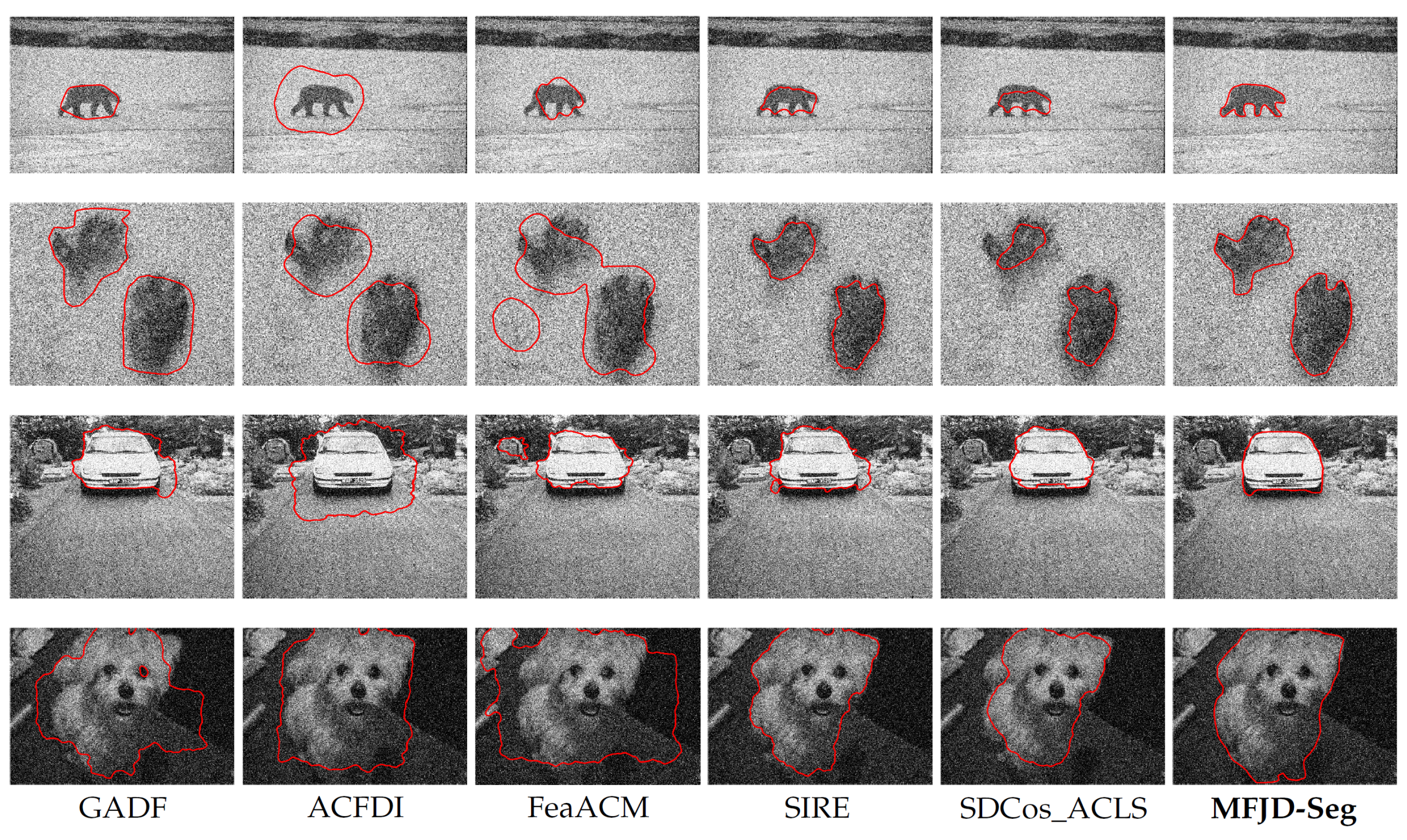
Figure 7.
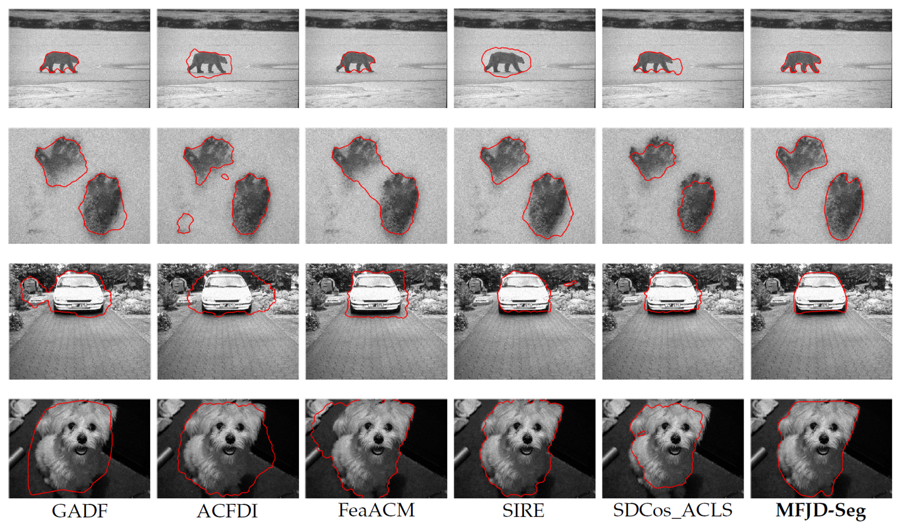
Examples of segmentation results for images with Gaussian noise.
Figure 7.
Examples of segmentation results for images with Gaussian noise.
Figure 8.
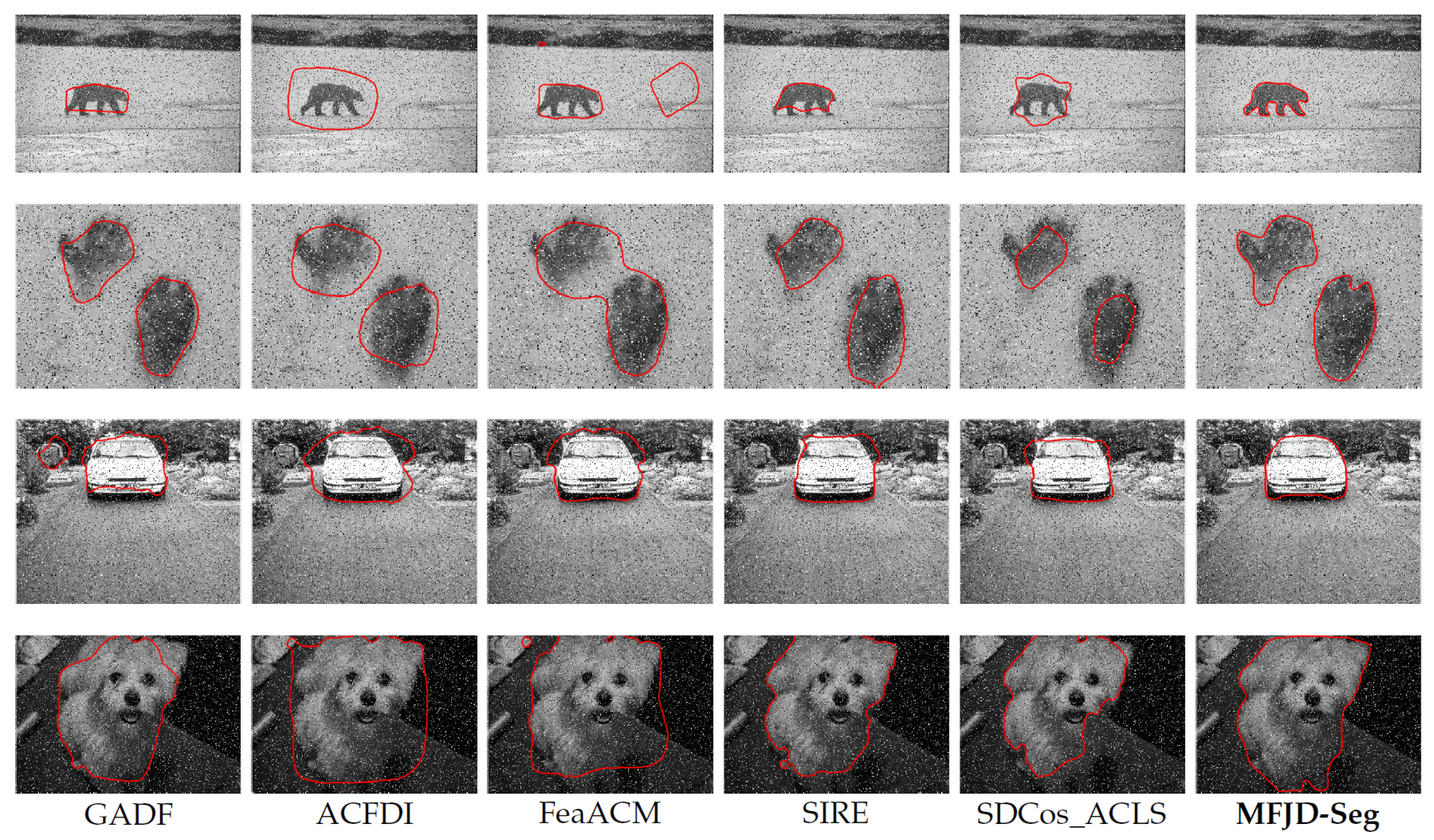
Examples of segmentation results for images with salt-and-pepper noise.
Figure 8.
Examples of segmentation results for images with salt-and-pepper noise.
Figure 9.
Examples of segmentation results for images with Poisson noise.
Figure 9.
Examples of segmentation results for images with Poisson noise.
Figure 10.
Visualization of for different ACMs.
Figure 10.
Visualization of for different ACMs.
Figure 11.
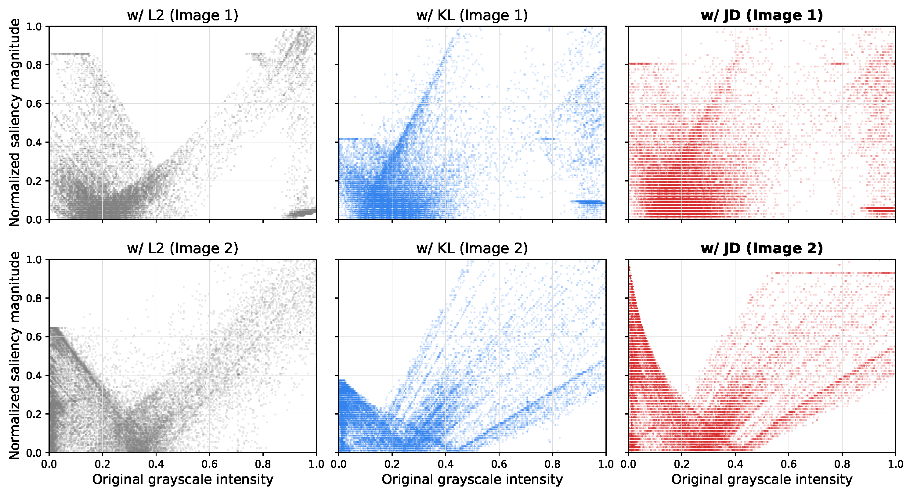
Pixel-level scatter comparison of different energy function formulations. The gray, blue, and red scatter points are generated based on the squared difference, KL divergence, and Jeffreys divergence, respectively.
Figure 11.
Pixel-level scatter comparison of different energy function formulations. The gray, blue, and red scatter points are generated based on the squared difference, KL divergence, and Jeffreys divergence, respectively.
Figure 12.
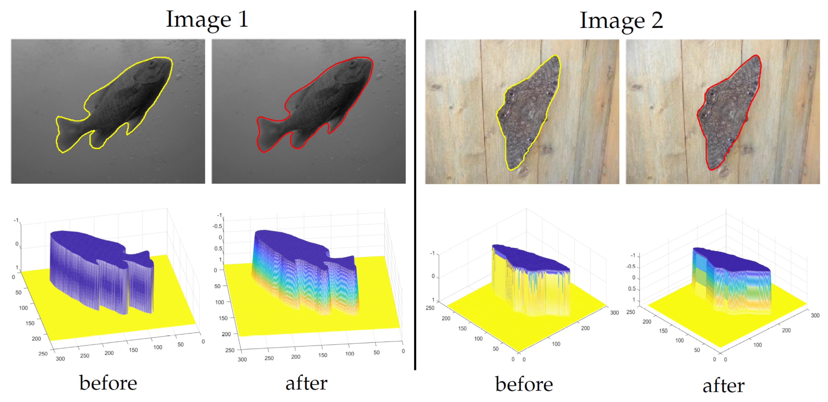
Qualitative comparison before and after applying mean filtering. Row 1: The 2D segmentation results. Row 2: The 3D level set functions. The yellow and red lines denote the segmentation results before and after filtering, respectively.
Figure 12.
Qualitative comparison before and after applying mean filtering. Row 1: The 2D segmentation results. Row 2: The 3D level set functions. The yellow and red lines denote the segmentation results before and after filtering, respectively.
Table 1.
Results of the comparative experiment with ACMs. The best performance is highlighted in bold.
Table 1.
Results of the comparative experiment with ACMs. The best performance is highlighted in bold.
| Method | BSDS | ADE20K | COCO |
|---|
| mIoU↑ | mDSC↑ | FPS↑ | mIoU↑ | mDSC↑ | FPS↑ | mIoU↑ | mDSC↑ | FPS↑ |
|---|
| GADF | 81.0 | 85.3 | 37.7 | 45.4 | 47.6 | 28.4 | 37.2 | 36.4 | 32.1 |
| ACFDI | 81.3 | 85.4 | 38.5 | 41.4 | 44.4 | 29.5 | 38.6 | 37.6 | 34.7 |
| FeaACM | 85.0 | 88.8 | 39.7 | 45.1 | 48.6 | 31.8 | 42.7 | 40.9 | 38.3 |
| SIRE | 77.7 | 84.6 | 46.3 | 47.6 | 50.9 | 39.2 | 36.5 | 37.3 | 41.1 |
| SDCos_ACLS | 82.4 | 87.3 | 42.4 | 47.3 | 50.0 | 34.4 | 41.3 | 39.0 | 37.4 |
| MFJD-Seg (Ours) | 89.7 | 93.4 | 50.7 | 52.4 | 55.6 | 43.8 | 47.5 | 45.7 | 45.4 |
Table 2.
Results of the comparative experiment with deep learning models. The best performance is highlighted in bold.
Table 2.
Results of the comparative experiment with deep learning models. The best performance is highlighted in bold.
| Method | BSDS | ADE20K | COCO |
|---|
| mIoU↑ | mDSC↑ | FPS↑ | mIoU↑ | mDSC↑ | FPS↑ | mIoU↑ | mDSC↑ | FPS↑ |
|---|
| SegFormer | 83.1 | 87.8 | 44.8 | 46.2 | 49.9 | 35.0 | 41.7 | 39.9 | 38.7 |
| U2Seg | 84.4 | 88.8 | 52.1 | 51.4 | 54.2 | 44.5 | 42.7 | 41.3 | 46.8 |
| E2EC | 86.1 | 89.9 | 46.0 | 47.7 | 51.1 | 37.2 | 44.1 | 42.2 | 40.8 |
| CGViT | 87.5 | 91.2 | 48.7 | 50.2 | 53.0 | 40.4 | 45.5 | 43.1 | 42.2 |
| EfficientViT | 88.6 | 92.1 | 51.5 | 49.0 | 52.1 | 45.2 | 46.2 | 44.2 | 46.1 |
| MFJD-Seg (Ours) | 89.7 | 93.4 | 50.7 | 52.4 | 55.6 | 43.8 | 47.5 | 45.7 | 45.4 |
Table 3.
Results of the comparative experiment with segmentation foundation models. The best performance is highlighted in bold.
Table 3.
Results of the comparative experiment with segmentation foundation models. The best performance is highlighted in bold.
| Method | BSDS | ADE20K | COCO |
|---|
| mIoU↑ | mDSC↑ | FPS↑ | mIoU↑ | mDSC↑ | FPS↑ | mIoU↑ | mDSC↑ | FPS↑ |
|---|
| SAM | 88.6 | 92.2 | 22.5 | 50.8 | 54.0 | 19.3 | 47.0 | 45.8 | 20.7 |
| TS-SAM | 90.3 | 93.6 | 17.1 | 53.2 | 56.1 | 14.9 | 49.1 | 47.0 | 16.0 |
| COD-SAM | 89.1 | 92.8 | 15.5 | 51.6 | 54.7 | 13.6 | 47.6 | 46.2 | 14.5 |
| MFJD-Seg (Ours) | 89.7 | 93.4 | 50.7 | 52.4 | 55.6 | 43.8 | 47.5 | 45.7 | 45.4 |
Table 4.
Comparison of algorithm complexity with ACMs. N denotes the maximum iteration number, P refers to the total number of pixels in the input image, and d represents the dimension of the feature maps generated during segmentation.
Table 4.
Comparison of algorithm complexity with ACMs. N denotes the maximum iteration number, P refers to the total number of pixels in the input image, and d represents the dimension of the feature maps generated during segmentation.
| Methods | Time Complexity | Space Complexity |
|---|
| GADF | | |
| ACFDI | | |
| FeaACM | | |
| SIRE | | |
| SDCos_ACLS | | |
| MFJD-Seg | | |
Table 5.
Comparison of algorithm complexity with deep learning models.
Table 5.
Comparison of algorithm complexity with deep learning models.
| Method | Params (M) | GPU Mem. (GB) | GFLOPs (G) |
|---|
| SegFormer | 24.20 | 1.82 | 62.41 |
| U2Seg | 44.50 | 3.25 | 180.64 |
| E2EC | 38.72 | 2.24 | 245.85 |
| CGViT | 124.60 | 4.06 | 255.77 |
| EfficientViT | 24.30 | 1.28 | 19.11 |
| SAM | 636.00 | 5.85 | 3851.43 |
| TS-SAM | 32.60 | 1.87 | 124.56 |
| COD-SAM | 647.20 | 6.23 | 3865.04 |
| MFJD-Seg | 0 | N/A | 1.22 |
Table 6.
Results of the noise segmentation experiment. The best performance is highlighted in bold.
Table 6.
Results of the noise segmentation experiment. The best performance is highlighted in bold.
| Method | BSDS | ADE20K | COCO |
|---|
| mIoU↑ | mDSC↑ | FPS↑ | mIoU↑ | mDSC↑ | FPS↑ | mIoU↑ | mDSC↑ | FPS↑ |
|---|
| Under Gaussian noise |
| GADF | 74.3 | 78.2 | 33.2 | 38.0 | 40.1 | 24.3 | 29.7 | 29.2 | 28.5 |
| ACFDI | 74.2 | 78.8 | 33.8 | 33.7 | 37.5 | 25.6 | 31.1 | 30.8 | 31.0 |
| FeaACM | 78.3 | 81.8 | 35.4 | 37.3 | 41.8 | 27.1 | 35.5 | 33.2 | 33.7 |
| SIRE | 71.0 | 77.3 | 42.6 | 41.1 | 43.9 | 34.7 | 29.3 | 30.5 | 36.5 |
| SDCos_ACLS | 74.7 | 80.5 | 38.3 | 40.0 | 42.3 | 30.7 | 34.1 | 31.2 | 33.1 |
| MFJD-Seg (Ours) | 85.1 | 88.6 | 47.2 | 48.1 | 51.1 | 41.3 | 43.2 | 41.0 | 43.0 |
| Under salt-and-pepper noise |
| GADF | 72.1 | 76.5 | 33.1 | 35.4 | 38.2 | 24.1 | 27.5 | 27.1 | 28.2 |
| ACFDI | 71.8 | 77.2 | 33.5 | 31.2 | 35.3 | 25.1 | 29.1 | 28.6 | 30.4 |
| FeaACM | 76.3 | 80.2 | 35.1 | 34.8 | 39.5 | 26.8 | 33.2 | 31.4 | 33.1 |
| SIRE | 69.4 | 75.1 | 42.1 | 38.5 | 41.2 | 34.2 | 27.3 | 28.4 | 36.2 |
| SDCos_ACLS | 72.5 | 78.9 | 38.1 | 37.6 | 40.2 | 30.4 | 31.8 | 29.5 | 32.5 |
| MFJD-Seg (Ours) | 83.4 | 89.1 | 46.8 | 45.9 | 49.2 | 41.5 | 41.2 | 39.4 | 42.7 |
| Under Poisson noise |
| GADF | 76.8 | 80.9 | 34.5 | 40.5 | 42.7 | 25.4 | 32.4 | 31.8 | 29.8 |
| ACFDI | 77.2 | 81.2 | 35.2 | 36.2 | 39.8 | 26.8 | 33.8 | 33.1 | 32.2 |
| FeaACM | 81.4 | 84.6 | 36.8 | 39.9 | 44.2 | 28.3 | 38.2 | 35.9 | 35.1 |
| SIRE | 73.6 | 80.1 | 44.2 | 43.8 | 46.5 | 36.3 | 31.9 | 33.4 | 38.2 |
| SDCos_ACLS | 77.5 | 83.2 | 39.9 | 42.7 | 45.1 | 32.1 | 36.9 | 34.2 | 34.6 |
| MFJD-Seg (Ours) | 88.5 | 92.3 | 49.1 | 51.2 | 54.4 | 42.6 | 45.8 | 43.9 | 44.5 |
Table 7.
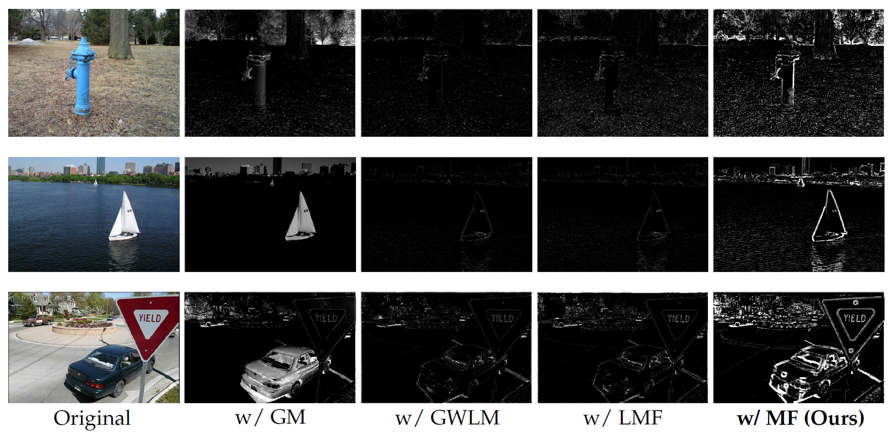
Ablation results of different image fitting algorithms. The best performance is highlighted in bold.
Table 7.
Ablation results of different image fitting algorithms. The best performance is highlighted in bold.
| Model | BSDS | ADE20K | COCO |
|---|
| mIoU↑ | mDSC↑ | mIoU↑ | mDSC↑ | mIoU↑ | mDSC↑ |
|---|
| w/GM | 84.9 | 88.7 | 46.7 | 49.0 | 40.6 | 38.3 |
| w/GWLM | 88.3 | 91.6 | 48.5 | 51.4 | 44.0 | 41.8 |
| w/LMF | 86.7 | 90.4 | 50.0 | 52.7 | 44.8 | 42.6 |
| w/MF (Ours) | 89.7 | 93.4 | 52.4 | 55.6 | 47.5 | 45.7 |
Table 8.
Ablation results of different energy function formulations. The best performance is highlighted in bold.
Table 8.
Ablation results of different energy function formulations. The best performance is highlighted in bold.
| Model | BSDS | ADE20K | COCO |
|---|
| mIoU↑ | mDSC↑ | mIoU↑ | mDSC↑ | mIoU↑ | mDSC↑ |
|---|
| w/ | 83.4 | 87.0 | 45.5 | 49.3 | 40.6 | 39.2 |
| w/KL | 86.3 | 90.1 | 49.1 | 52.0 | 43.9 | 42.1 |
| w/JD (Ours) | 89.7 | 93.4 | 52.4 | 55.6 | 47.5 | 45.7 |
Table 9.
Ablation results of the energy constraint term. The best performance is highlighted in bold.
Table 9.
Ablation results of the energy constraint term. The best performance is highlighted in bold.
| Model | BSDS | ADE20K | COCO |
|---|
| mIoU↑ | mDSC↑ | mIoU↑ | mDSC↑ | mIoU↑ | mDSC↑ |
|---|
| w/o energy constraint | 86.3 | 90.6 | 47.7 | 51.1 | 42.3 | 41.1 |
| w/energy constraint | 89.7 | 93.4 | 52.4 | 55.6 | 47.5 | 45.7 |
Table 10.
Ablation results of the mean filtering module. The best performance is highlighted in bold.
Table 10.
Ablation results of the mean filtering module. The best performance is highlighted in bold.
| Model | BSDS | ADE20K | COCO |
|---|
| mIoU↑ | mDSC↑ | mIoU↑ | mDSC↑ | mIoU↑ | mDSC↑ |
|---|
| w/o mean filtering | 87.8 | 91.5 | 51.0 | 53.0 | 45.2 | 44.4 |
| w/mean filtering | 89.7 | 93.4 | 52.4 | 55.6 | 47.5 | 45.7 |
Table 11.
Performance of MFJD-Seg under different . The best performance is highlighted in bold.
Table 11.
Performance of MFJD-Seg under different . The best performance is highlighted in bold.
| BSDS | ADE20K | COCO |
|---|
| mIoU↑ | mDSC↑ | mIoU↑ | mDSC↑ | mIoU↑ | mDSC↑ |
|---|
| 10 | 87.1 | 89.6 | 47.7 | 49.9 | 42.4 | 41.7 |
| 13 | 88.9 | 92.3 | 51.3 | 54.1 | 46.1 | 45.0 |
| 15 | 89.7 | 93.4 | 52.4 | 55.6 | 47.5 | 45.7 |
| 17 | 89.1 | 92.1 | 50.8 | 53.7 | 45.9 | 44.6 |
| 20 | 86.4 | 89.0 | 47.0 | 49.3 | 42.0 | 41.1 |
Table 12.
Performance of MFJD-Seg under different k. The best performance is highlighted in bold.
Table 12.
Performance of MFJD-Seg under different k. The best performance is highlighted in bold.
| k | BSDS | ADE20K | COCO |
|---|
| mIoU↑ | mDSC↑ | mIoU↑ | mDSC↑ | mIoU↑ | mDSC↑ |
|---|
| 3 | 87.5 | 90.9 | 49.1 | 51.4 | 43.9 | 42.6 |
| 5 | 89.3 | 92.7 | 51.7 | 54.7 | 46.6 | 45.3 |
| 7 | 89.7 | 93.4 | 52.4 | 55.6 | 47.5 | 45.7 |
| 9 | 89.0 | 92.5 | 51.4 | 54.3 | 46.3 | 45.1 |
| 11 | 87.2 | 90.3 | 48.3 | 50.8 | 43.2 | 42.0 |
Table 13.
Performance of MFJD-Seg under different . The best performance is highlighted in bold.
Table 13.
Performance of MFJD-Seg under different . The best performance is highlighted in bold.
| BSDS | ADE20K | COCO |
|---|
| mIoU↑ | mDSC↑ | mIoU↑ | mDSC↑ | mIoU↑ | mDSC↑ |
|---|
| 0.02 | 86.6 | 89.4 | 46.9 | 49.6 | 41.5 | 41.0 |
| 0.05 | 88.5 | 92.0 | 50.3 | 53.3 | 45.3 | 43.9 |
| 0.1 | 89.7 | 93.4 | 52.4 | 55.6 | 47.5 | 45.7 |
| 0.2 | 87.2 | 90.3 | 48.0 | 50.7 | 43.2 | 42.2 |
| 0.3 | 84.1 | 86.7 | 42.4 | 45.4 | 37.6 | 37.6 |
Table 14.
Performance of MFJD-Seg under different N. The best performance is highlighted in bold.
Table 14.
Performance of MFJD-Seg under different N. The best performance is highlighted in bold.
| N | BSDS | ADE20K | COCO |
|---|
| mIoU↑ | mDSC↑ | mIoU↑ | mDSC↑ | mIoU↑ | mDSC↑ |
|---|
| 20 | 87.4 | 90.3 | 47.4 | 50.3 | 42.0 | 41.3 |
| 35 | 88.5 | 92.2 | 50.7 | 53.6 | 44.9 | 42.6 |
| 50 | 89.7 | 93.4 | 52.4 | 55.6 | 47.5 | 45.7 |
| 60 | 89.3 | 93.3 | 52.3 | 55.5 | 47.4 | 45.6 |
| 70 | 89.4 | 93.2 | 52.2 | 55.4 | 47.3 | 45.6 |