A Physics-Aware Dual-Branch CNN-MLP Fusion Framework for Stage-Aware Bearing Degradation Monitoring and RUL Prognosis from Vibration Signals

Abstract

Rolling element bearing degradation monitoring is critical for predictive maintenance in rotating machinery systems. Existing methods predominantly address fault classification and remaining useful life (RUL) estimation as separate tasks, thereby failing to capture the progressive and multistage nature of bearing deterioration. This paper proposes a physics-aware multi-modal fusion framework for continuous RUL prediction from vibration signals, organized around a stage-aware representation of the bearing life cycle. The proposed pipeline integrates two complementary preprocessing branches: Hilbert envelope demodulation followed by short-time Fourier transform (STFT) to generate degradation-sensitive time–frequency spectrograms, and handcrafted statistical feature extraction to yield compact global severity descriptors. A dual-head convolutional neural network-multilayer perceptron (CNN-MLP) architecture is designed to learn discriminative representations from both modalities and fuse them for end-to-end normalized RUL regression. The bearing life cycle is further partitioned into four ordered degradation stages based on normalized life–progress ratios, providing an interpretable health representation that complements the continuous prognosis target. Experiments conducted on the PRONOSTIA/FEMTO-ST benchmark dataset demonstrate that the proposed framework achieves an RMSE of 0.1597, an MAE of 0.1328, and an $R^2$ of 0.7487 on normalized RUL prediction, with stable error behavior across most of the life cycle. Feature importance analysis confirms that the CNN branch captures localized low-to-mid-frequency spectral evolution while the MLP branch encodes amplitude variability and impulsive indicators, validating the complementarity of the dual-branch design. The proposed method offers a unified, interpretable, and engineering-relevant solution for intelligent bearing condition monitoring and prognostic health management.

1. Introduction

1.1. Research Background and Motivation

Rolling element bearings are indispensable components in rotating machinery and are widely used in industrial motors, gearboxes, turbines, and automated manufacturing equipment [1]. Their health condition directly affects the operational reliability, maintenance cost, and safety of electromechanical systems [2]. Once bearing degradation evolves from incipient damage to severe failure, it may induce abnormal vibration, efficiency loss, unplanned shutdowns, and even cascading faults across the entire system [3,4]. Accurate health monitoring and early prognosis of bearing degradation have therefore become essential in intelligent industrial electronics and predictive maintenance applications.

With the rapid development of sensing technology, embedded monitoring devices, and data-driven analytics, vibration-based condition monitoring has become one of the most effective approaches for bearing health assessment. Compared with periodic manual inspection, online monitoring based on sensor signals can provide continuous information on degradation evolution and support timely maintenance decisions. In particular, vibration signals are highly sensitive to local defects such as pitting, spalling, and raceway damage, which makes them suitable for fault diagnosis and degradation tracking [3,5,6]. However, raw vibration responses are typically non-stationary, noise-contaminated, and strongly coupled with operating conditions, making robust feature extraction and life prediction difficult [7].

Recent advances in machine learning and deep learning have substantially improved intelligent fault diagnosis and prognosis [4,8]. Convolutional neural networks have demonstrated strong capability for extracting local fault patterns from vibration signals and spectrogram representations [9,10,11]. Recurrent architectures, including long short-term memory networks and gated recurrent units, have been widely adopted for temporal degradation modeling and RUL estimation due to their ability to capture sequential health evolution [12,13]. Attention-based and transformer-derived models have further advanced prognostic performance by enabling adaptive, long-range feature interactions within degradation sequences [4,14]. However, many existing studies focus either on fault classification or on remaining useful life (RUL) regression alone [14,15]. In practical industrial scenarios, bearing degradation is a progressive process rather than an abrupt state transition. From a maintenance perspective, it is not sufficient to determine whether a bearing is healthy or faulty; the degradation stage and the remaining service life are both required. This motivates the development of a unified framework that can simultaneously characterize multistage degradation behavior and provide reliable RUL prognosis.

1.2. Literature Gap and Problem Statement

Existing bearing monitoring methods can generally be divided into signal-processing-based approaches and data-driven learning approaches. Traditional signal analysis methods, such as envelope analysis, spectral analysis, wavelet transform, and time–frequency decomposition, are effective in highlighting physically meaningful fault signatures [5,6,16]. Their main strength lies in interpretability, since characteristic frequencies and impulsive components can often be associated with specific defect mechanisms. However, these methods usually rely on hand-crafted features and expert knowledge, which limits adaptability under varying operating conditions and complex degradation trajectories [7,16].

Deep learning methods reduce the dependence on manual feature engineering by automatically learning discriminative representations from raw or transformed signals [8,10]. CNN-based models can extract localized patterns from time–frequency images, while sequence models are effective in capturing temporal dependencies in degradation processes [9,11]. More recent multimodal architectures attempt to combine heterogeneous features for improved performance [17]. However, several limitations remain.

Many studies still treat bearing monitoring as a single-task problem [4,14,15]. Fault diagnosis is often formulated as a discrete classification task, whereas prognosis is typically formulated as a continuous regression task [18,19]. Such isolated formulations do not fully reflect the progressive nature of bearing degradation. In practice, degradation stage recognition improves interpretability and maintenance awareness, whereas RUL estimation provides quantitative support for maintenance scheduling. A framework that combines both is therefore more consistent with real operational requirements.

Purely data-driven models also tend to underuse physical signal characteristics [4,20]. In bearing vibration analysis, defect-induced impulsive modulation is one of the most informative mechanisms underlying degradation evolution [3,5]. If such prior knowledge is not incorporated into preprocessing or feature construction, the learned representation may become less robust under noisy conditions or limited sample sizes.

Single-modal learning further constrains degradation modeling [14]. Time–frequency representations can reveal local spectral evolution and fault-related modulation patterns, but they do not always provide a compact description of global degradation severity. By contrast, statistical indicators such as root mean square, kurtosis, crest factor, and standard deviation summarize energy, impulsiveness, and dispersion characteristics [6,21], but they may overlook fine-grained spectral structure. A framework that jointly exploits these complementary properties is therefore desirable.

Accordingly, the main problem addressed in this study is how to construct a physics-aware and multi-modal deep learning framework for bearing health monitoring that can effectively extract degradation-sensitive information from raw vibration signals, represent both stage-wise degradation characteristics and continuous life evolution, and provide accurate and interpretable RUL prediction for intelligent monitoring systems. The proposed framework is subsequently evaluated on the publicly available PRONOSTIA/FEMTO-ST benchmark [4], which enables direct quantitative comparison with independently published methods working on the same dataset—a prerequisite for rigorously assessing the method’s value relative to the state of the art.

1.3. Main Contributions

This paper proposes a physics-aware multi-modal framework for multistage bearing degradation diagnosis and RUL prognosis. The main contributions are summarized as follows.

• Stage-aware RUL prognosis framework. A single end-to-end pipeline is developed that predicts continuous normalized RUL using a stage-aware health representation. The bearing life cycle is partitioned into four ordered degradation stages based on normalized life–progress ratios; these stage labels organize the degradation trajectory into interpretable health regions and support stage-dependent performance analysis, but the sole model prediction target is the normalized RUL. This design makes model behavior more transparent and maintenance-relevant without requiring a separate classification head or loss term.
• Deliberate physics-aware preprocessing chain. Rather than applying time–frequency analysis directly to raw vibration, Hilbert envelope demodulation is first applied to isolate the amplitude-modulated fault component, and STFT is subsequently applied to the envelope signal. This two-step chain exploits the physical mechanism of defect-induced impulsive modulation to enhance degradation sensitivity before any learning takes place, as demonstrated by the clear spectral redistribution visible between healthy and degraded spectrograms.
• Complementary dual-branch architecture with ablation validation. A CNN branch processes the physics-enhanced 2-D spectrogram to capture localized time–frequency patterns, while a parallel MLP branch encodes a 783-dimensional handcrafted feature vector summarizing global signal severity. Both branches are trained end-to-end with ${\mathcal{l}}_2$ regularization, and their concatenated embeddings are directly optimized for RUL regression. Ablation experiments reported in Section 4 confirm that neither branch alone matches the joint model, quantitatively validating the complementary value of each modality rather than merely assuming it.
• Experimental validation and engineering analysis. The framework is evaluated on the PRONOSTIA/FEMTO-ST benchmark with detailed error analysis, feature-importance attribution, and stage-dependent performance breakdown, providing both quantitative performance evidence and interpretable insight for intelligent bearing condition monitoring.

1.4. Organization of the Paper

The remainder of this paper is organized as follows.

Section 2 reviews related works on bearing signal processing, deep learning for condition monitoring, and multistage degradation modeling with RUL prediction.

Section 3 presents the proposed methodology, including dataset description, physics-aware signal preprocessing, multistage degradation modeling, and the dual-branch CNN–MLP feature-level fusion network.

Section 4 reports the experimental settings and results, including prognostic performance, comparative evaluation, ablation analysis, and deployment-oriented discussion.

Section 5 discusses the effectiveness, engineering implications, and limitations of the proposed framework, concludes the paper and outlines future research directions.

2. Related Works

2.1. Signal Processing Methods for Bearing Monitoring

Signal processing has long been a fundamental approach in bearing condition monitoring because bearing defects usually manifest as localized impulses, amplitude modulation, and characteristic frequency components in vibration signals [5,22]. Classical methods such as time-domain statistical analysis, frequency-domain spectral analysis, and envelope demodulation have been widely used to reveal degradation-related signatures [21]. Indicators including root mean square, kurtosis, crest factor, skewness, and peak-to-peak value are commonly adopted to characterize energy variation, impulsiveness, and waveform distortion during the degradation process [6]. These features provide a compact description of signal behavior and remain attractive in practical monitoring systems due to their simplicity and low computational cost.

Frequency-domain analysis further enhances defect identification by linking spectral peaks to specific fault frequencies associated with the inner race, outer race, rolling elements, or cage [16]. However, bearing vibration signals are typically non-stationary, especially under variable operating conditions and progressive damage evolution [7]. In such cases, purely stationary spectral analysis may be insufficient to capture transient fault signatures. To address this issue, time–frequency methods such as short-time Fourier transform, wavelet transform, empirical mode decomposition, and Hilbert–Huang transform have been introduced to better represent the temporal evolution of defect-related components [23]. These methods provide richer descriptions of local spectral changes and are particularly useful in early degradation analysis.

Among existing signal-processing approaches, envelope analysis remains especially important in bearing diagnosis because many localized defects generate repetitive impacts that excite structural resonances [24]. Hilbert-based envelope demodulation can effectively extract the modulated low-frequency fault information from high-frequency carrier components, thereby improving the visibility of defect patterns. This characteristic makes it highly suitable for degradation-sensitive preprocessing. However, traditional signal-processing pipelines still depend heavily on manual feature design and prior expertise. Their performance can degrade when the operating environment changes or when multiple degradation patterns overlap. As a result, signal processing alone may not be sufficient for robust multistage degradation modeling and long-horizon life prediction.

2.2. Deep Learning Methods for Fault Diagnosis and Prognosis

Deep learning has significantly changed the paradigm of bearing health monitoring by enabling automatic feature learning from raw signals or transformed representations [8,10]. Convolutional neural networks have been extensively used for fault diagnosis because of their strong ability to capture local structures in one-dimensional vibration sequences or two-dimensional time–frequency images. By stacking convolution and pooling operations, CNN-based models can learn increasingly abstract fault-related features without relying entirely on handcrafted descriptors [9,11]. This advantage has made CNNs one of the most frequently adopted architectures in rotating machinery diagnosis.

Recurrent neural networks, particularly long short-term memory and gated recurrent unit models, have also been introduced for degradation analysis and prognosis [12]. Their main strength lies in modeling sequential dependencies and temporal evolution, which is valuable for predicting the progression of system health states over time. For RUL estimation, such temporal learning capability is especially relevant because degradation is inherently dynamic [13]. More recently, transformer-based and attention-enhanced architectures have attracted growing interest due to their ability to capture long-range dependencies and adaptive feature interactions. These models have shown promising performance in both diagnosis and prognosis tasks, especially when sufficient data and computational resources are available [8].

Despite these advances, several challenges remain. Many deep learning studies prioritize predictive accuracy while paying limited attention to physical interpretability. End-to-end models trained directly on raw data can behave as black boxes, which reduces transparency in maintenance decision-making [20]. In addition, pure deep models often require large-scale labeled datasets and may become sensitive to noise, domain shifts, or class imbalance. This issue is particularly relevant in bearing monitoring, where degradation data near failure are relatively scarce and health-state transitions are often gradual rather than sharply separable. Overall, existing deep learning methods have demonstrated strong representation power, but more effective integration of domain knowledge and complementary feature modalities is still needed for robust and interpretable prognosis.

2.3. Multistage Degradation Modeling and RUL Prediction

Remaining useful life prediction has become a central topic in prognostics and health management because it directly supports maintenance scheduling and failure prevention [4]. Existing RUL prediction methods can generally be categorized into model-based, statistical, and data-driven approaches. Model-based methods attempt to describe degradation dynamics through physical or stochastic processes, while data-driven methods learn degradation patterns from historical monitoring data. With the increasing availability of sensor measurements, data-driven RUL prediction has become the dominant research direction in bearing prognosis [15].

Most existing RUL studies formulate the problem as continuous regression and aim to predict the distance between the current health condition and the failure threshold [18]. This formulation is effective for quantitative prognosis, but it does not always provide sufficient interpretability regarding how degradation evolves across different life stages. In practice, maintenance decisions are often not triggered solely by an estimated remaining lifetime; they are also influenced by whether the system is in a healthy, incipient, intermediate, or severe degradation stage. Stage-aware modeling therefore provides an important intermediate layer between raw signals and continuous lifetime prediction.

Several studies have attempted to bridge diagnosis and prognosis through health index construction, degradation trend extraction, or state partitioning methods [19]. Health indices derived from statistical features, deep latent representations, or reconstruction errors can reflect the gradual deterioration of bearings and support downstream RUL estimation. Change-point detection and stage division strategies have also been used to identify transitions between health states. However, these methods are often implemented as separate modules rather than as components of a unified framework. Moreover, some stage partitioning approaches rely on heuristic thresholds that may not generalize well across datasets and operating conditions.

Another limitation is that many RUL prediction models rely on a single representation space [14]. Methods based only on statistical features may overlook detailed local fault patterns, while methods based only on time–frequency images may not fully capture compact global degradation trends. Since multistage degradation and RUL prediction are closely related but not identical tasks, a joint representation that combines physically meaningful signal features with learned deep representations is more suitable for describing the full degradation process.

2.4. Summary and Research Positioning

The existing literature demonstrates that both signal processing and deep learning contribute substantially to bearing condition monitoring. Signal-processing-based methods offer clear physical interpretability and can effectively expose defect-related components, especially through demodulation and time–frequency analysis. Deep learning methods, by contrast, provide strong representation capability and reduce dependence on manual feature engineering. However, neither direction fully resolves the combined challenge of multistage degradation characterization and continuous RUL prediction.

Current studies still exhibit several gaps. On the one hand, many diagnosis methods remain focused on discrete fault recognition rather than progressive degradation understanding. On the other hand, many prognosis methods treat RUL estimation as a pure regression problem and do not explicitly incorporate degradation stages. In addition, purely data-driven models often underuse known fault mechanisms, whereas purely handcrafted feature approaches may fail to capture complex nonlinear degradation patterns. This separation limits both predictive robustness and practical interpretability.

Against this background, the present study is positioned as a unified diagnosis–prognosis framework for bearing degradation monitoring. The proposed method combines physics-aware preprocessing and multi-modal deep feature fusion within a single pipeline. Hilbert envelope demodulation and STFT-based spectrogram generation are used to preserve degradation-sensitive signal characteristics, while statistical indicators are introduced to describe global degradation severity. A dual-head CNN-MLP architecture is then employed to jointly learn complementary features for multistage degradation representation and RUL prediction. In this sense, the present work aims to connect physical signal understanding, deep representation learning, and engineering-oriented prognostic modeling in a more coherent manner.

To clarify the research positioning of the present study,

Table 1. Qualitative capability comparison across representative methodological streams in bearing degradation monitoring and prognosis. Checkmarks indicate that the capability is a primary characteristic of the stream; “partial” indicates it is addressed in a subset of methods or in a limited form. A quantitative performance comparison on the PRONOSTIA/FEMTO-ST benchmark is provided separately in Section 4.

Study (Ref.)	Physics-Aware Preprocessing	Statistical Feature Repr.	Deep Repr. Learning	Multistage Degr. Model	Continuous RUL Pred.	Interpretability
Signal-processing [5,6,7,24]	✓	partial	–	–	–	✓
Handcrafted-feature [16,21]	partial	✓	–	–	–	✓
Deep-learning [4,12,13,20]	partial	partial	✓	partial	partial	partial
RUL-oriented [14,15,18,19]	partial	partial	partial	partial	✓	partial
Guo et al. [17]	partial	✓	✓	partial	✓	partial
This work	✓	✓	✓	✓	✓	✓

provides a qualitative comparison across representative methodological streams in bearing degradation monitoring and prognosis. This table characterizes the capability coverage of each stream at a feature level and is intended to establish methodological positioning; it is complemented by the quantitative performance comparison against published methods on the PRONOSTIA/FEMTO-ST benchmark provided in Section 4.

As shown in Table 1, existing studies usually emphasize only part of the bearing monitoring problem, such as physics-based fault enhancement, handcrafted condition description, deep feature learning, or RUL-oriented prognosis. In contrast, the present study integrates physics-aware preprocessing, statistical and deep feature fusion, stage-aware degradation representation, and continuous RUL prediction within a unified framework.

Among the most closely related works, Guo et al. [17] propose a hybrid prognosis scheme that constructs a novel health indicator via Complete Ensemble Empirical Mode Decomposition with Adaptive Noise and Kernel Principal Component Analysis, and subsequently models degradation through a nonlinear Wiener process for RUL prediction. That study demonstrates the value of combining data-driven health indicator construction with probabilistic degradation modeling. The present framework differs in two key respects: first, physics-aware Hilbert envelope demodulation is applied as a deliberate preprocessing step to isolate defect-induced modulation before any learning takes place, rather than relying on an unsupervised decomposition to construct a health indicator post hoc; second, a joint CNN–MLP fusion architecture simultaneously learns stage-wise degradation classification and continuous RUL regression in a single end-to-end pipeline, whereas the approach in [17] separates health indicator construction from the probabilistic prognosis model.

3. Materials and Methods

3.1. Dataset and Overall Framework

3.1.1. Dataset Description

To evaluate the proposed multistage bearing degradation diagnosis and prognosis framework, this study employs the PRONOSTIA bearing dataset, also referred to as the FEMTO-ST dataset, originally introduced in the IEEE PHM 2012 Prognostics Challenge. This dataset is widely used in prognostics and health management because it records the full degradation-to-failure process of rolling bearings under controlled operating conditions. The experiments were conducted on the PRONOSTIA platform, where bearings were operated under accelerated degradation conditions until failure. Such a configuration is particularly suitable for studying both degradation-stage evolution and remaining useful life prediction.

The dataset provides multi-sensor measurements collected throughout the entire life cycle of each bearing. In the original acquisition setting, two vibration channels, corresponding to horizontal and vertical accelerometers, were sampled at 25.6 kHz, while the temperature signal was sampled at 10 Hz. For each acquisition instant, a vibration snapshot with a duration of 0.1 s was recorded every 10 s. Since the vibration sampling frequency is 25.6 kHz, each raw vibration snapshot contains

$$N=f_s\times T=\mathrm{25,600}\times 0.1=2560$$

(1)

sampling points, where $f_s$ is the sampling frequency and T is the acquisition duration. This sample length preserves sufficient high-frequency fault information while keeping the storage and computation burden within a manageable range.

In the present study, each signal snapshot is treated as a basic observation unit. After preprocessing and feature extraction, the raw time-series sample is transformed into structured learning inputs.

To construct the fixed-size sample set from the full bearing life-cycle trajectories, a uniform temporal subsampling strategy is applied. The PRONOSTIA dataset partitions its bearings into a learning set and a test set at the bearing level: bearings in the learning set are used for model training, and bearings in the test set are reserved for evaluation. Each bearing’s life-cycle trajectory consists of a varying number of sequential snapshots depending on its total run-to-failure duration. To ensure balanced representation of all degradation stages and to maintain a fixed sample count per bearing, snapshots are selected at equally spaced indices along each bearing’s full temporal sequence. Specifically, $N_{\mathrm{train}}$ snapshots are selected from each training bearing and $N_{\mathrm{test}}$ snapshots from each test bearing, yielding a training set of 500 samples across the training bearings and a test set of 100 samples across the test bearings. No data augmentation or cross-bearing overlap is applied; the train/test split is strictly bearing-level to prevent information leakage. The resulting dataset therefore contains one sample per selected snapshot, with each sample independently processed through the same preprocessing and feature extraction pipeline described in Section 3.2.

To improve the clarity of the dataset description, the key information can be summarized as shown in

Table 2. Summary of the dataset and processed samples.

Item	Description
Dataset	IEEE PHM 2012/FEMTO-ST (PRONOSTIA)
Platform	PRONOSTIA accelerated bearing degradation platform
Sensor channels	Horizontal vibration, vertical vibration, temperature
Vibration sampling frequency	25.6 kHz
Temperature sampling frequency	10 Hz
Snapshot duration	0.1 s
Snapshot interval	10 s
Raw points per vibration snapshot	2560
Processed sample size	500 samples
Input feature dimension	783
Test sample size	100 samples

.

To provide additional context on the experimental conditions, Figure 1 presents a schematic overview of the PRONOSTIA/FEMTO-ST bearing degradation test platform and the associated signal processing pipeline. In the test configuration (upper portion of the figure), a constant-speed motor drives a rotating shaft on which the test bearing is mounted. A radial load system applies a constant downward force to the bearing, imposing accelerated degradation conditions. An accelerometer mounted on the bearing housing captures vibration signals, which are routed through a data acquisition system and stored for offline analysis. The acquisition protocol records a 0.1 s vibration snapshot at 25.6 kHz every 10 s, continuing automatically until the predefined failure threshold is exceeded. The lower portion of the figure summarizes the signal processing chain adopted in the present study: raw vibration snapshots are first segmented into fixed-length windows, then processed through Hilbert envelope demodulation and STFT to generate spectrograms, followed by handcrafted statistical feature extraction, and finally input to the RUL prediction model.

Compared with conventional static fault datasets, this dataset is more suitable for life-cycle prognostic modeling because it records the gradual transition from healthy operation to severe degradation and failure. This property enables the construction of both stage-wise degradation labels and continuous RUL labels.

3.1.2. Problem Definition

This study formulates bearing health monitoring as a prognostic regression problem with stage-aware data organization. Let $\mathbf{x}\left(t_i\right)$ denote the raw vibration signal at the i-th acquisition instant, where $i=1,2,\dots ,N$. The primary objective is to learn a mapping from the raw observation to the normalized remaining useful life:

$$f:\mathbf{x}\left(t_i\right)\to {\widetilde{\mathrm{RUL}}}_i$$

(2)

To provide interpretable structure for the degradation trajectory, the full bearing life cycle is additionally partitioned into ordered health stages used for data labeling and analysis:

$$\mathcal{S}=\{S_1,S_2,\dots ,S_K\}$$

(3)

where K denotes the number of degradation stages. In this work, a four-stage setting is adopted, corresponding to healthy, early degradation, intermediate degradation, and severe degradation. These stage labels are used to organize the life-cycle trajectory into interpretable health regions and to support stage-dependent performance analysis; they do not constitute a separate model output.

For RUL prediction, let $T_f$ denote the failure time index and $t_i$ denote the current observation index. The raw remaining useful life is defined as

$${\mathrm{RUL}}_i=T_f-t_i$$

(4)

Because different bearings may have different life spans, direct regression on ${\mathrm{RUL}}_i$ may introduce scale inconsistency across bearings. To improve comparability and training stability, a normalized RUL target is adopted:

$${\widetilde{\mathrm{RUL}}}_i={\displaystyle \frac{T_f-t_i}{T_f}}$$

(5)

which maps the full life cycle into the interval $[0, 1]$, where values close to 1 indicate an early-life condition and values close to 0 indicate proximity to failure.

Accordingly, the learning problem can be expressed as

$${\widehat{y}}_i=g\left(\mathbf{S}\left({\mathbf{x}}_i\right),{\mathbf{f}}_{\mathrm{stat}}\left({\mathbf{x}}_i\right);\theta \right)$$

(6)

where $\mathbf{S}\left({\mathbf{x}}_i\right)$ denotes the time–frequency representation extracted from the signal, and ${\mathbf{f}}_{\mathrm{stat}}\left({\mathbf{x}}_i\right)$ denotes the corresponding statistical feature vector. This formulation preserves degradation continuity through normalized RUL regression, while the accompanying stage-aware labeling provides an interpretable organizational structure for performance analysis and health representation across the full life cycle.

3.1.3. Overall Workflow

The proposed framework contains four sequential modules: raw signal acquisition, physics-aware signal transformation, multi-modal feature construction, and deep fusion-based prediction. The full pipeline is illustrated in Figure 2.

At the signal level, the raw vibration sequence $\mathbf{x}\left(t\right)$ contains degradation-sensitive information but is also affected by noise, non-stationarity, and operating-condition variation. Directly feeding $\mathbf{x}\left(t\right)$ into a prediction model may obscure fault-related impulsive behavior. To address this issue, Hilbert envelope demodulation is first applied to extract the amplitude-modulated component associated with repeated defect impacts. The resulting envelope signal is then transformed by short-time Fourier transform into a two-dimensional spectrogram. In parallel, a set of statistical descriptors is extracted to characterize the global degradation pattern.

Formally, the transformation path can be written as

$$\mathbf{x}\left(t\right)\stackrel{\mathrm{Hilbert}}{\to }e\left(t\right)\stackrel{\mathrm{STFT}}{\to }\mathbf{S}(t,f)$$

(7)

for the time–frequency branch, and

$$\mathbf{x}\left(t\right)\to {\mathbf{f}}_{\mathrm{stat}}=[\mu ,\sigma ,\mathrm{RMS},\mathrm{Kurt},\mathrm{CF},\mathrm{PtP}]$$

(8)

for the statistical branch, where $e\left(t\right)$ is the envelope signal, $\mathbf{S}(t,f)$ is the spectrogram, and ${\mathbf{f}}_{\mathrm{stat}}$ is the handcrafted feature vector.

The final prediction model learns a joint mapping

$$\widehat{y}=h\left({\varphi }_{\mathrm{CNN}}\left(\mathbf{S}\right),{\varphi }_{\mathrm{MLP}}\left({\mathbf{f}}_{\mathrm{stat}}\right);\mathrm{\Theta }\right)$$

(9)

where ${\varphi }_{\mathrm{CNN}}$ denotes the feature extractor for the spectrogram branch, ${\varphi }_{\mathrm{MLP}}$ denotes the feature extractor for the statistical branch, and h denotes the fusion and output function.

3.2. Physics-Aware Signal Processing and Feature Construction

3.2.1. Hilbert Envelope Demodulation

Bearing surface defects usually generate repetitive impacts during rolling contact. These impacts excite high-frequency structural resonances, while the repetition rate is governed by defect-related kinematics. As a result, the useful degradation information is often embedded in an amplitude-modulated vibration signal [3,7].

As shown in Figure 3, the raw healthy and degraded signals exhibit substantial overlap in the time domain, and the degradation-related difference is not sufficiently explicit at the waveform level. This observation motivates the use of physics-aware preprocessing to enhance defect-sensitive modulation information.

If the raw waveform is written as a modulated resonance response,

$$x\left(t\right)=a\left(t\right)\cos (2\pi f_{c}t+\phi \left(t\right))$$

(10)

where $a\left(t\right)$ is the slowly varying modulation envelope, $f_c$ is the carrier resonance frequency, and $\phi \left(t\right)$ is the phase term, then the prognostically relevant fault information is primarily carried by $a\left(t\right)$, not by the rapidly oscillating carrier itself.

To recover $a\left(t\right)$, the analytic signal is constructed using the Hilbert transform:

$$z\left(t\right)=x\left(t\right)+j\mathcal{H}\left\{x\right(t\left)\right\}$$

(11)

where $\mathcal{H}\left\{x\right(t\left)\right\}$ is the Hilbert transform of $x\left(t\right)$,

$$\mathcal{H}\left\{x\left(t\right)\right\}={\displaystyle \frac{1}{\pi }}\mathrm{P}.\mathrm{V}.{\int }_{-\infty }^{\infty }{\displaystyle \frac{x\left(\tau \right)}{t-\tau }}d\tau$$

(12)

Substituting the modulated form $x\left(t\right)$ into the analytic representation yields

$$z\left(t\right)\approx a\left(t\right)e^{j(2\pi f_{c}t+\phi \left(t\right))}$$

(13)

Taking the magnitude of the analytic signal gives

$$e\left(t\right)=\left|z\right(t\left)\right|\approx a\left(t\right)$$

(14)

This derivation shows that the Hilbert envelope operation suppresses the fast carrier oscillation and isolates the slowly varying modulation component caused by repeated defect impacts. In bearing monitoring, this is important because early-stage degradation often appears as weak but periodic impulsive modulation rather than as a dominant amplitude increase in the raw signal.

From a signal-processing perspective, the envelope signal $e\left(t\right)$ provides a more fault-sensitive intermediate representation. From a prognostic perspective, it increases the visibility of degradation evolution before severe failure occurs. Therefore, Hilbert demodulation is used in this work as a physics-aware enhancement step before time–frequency transformation and feature extraction [7,25].

3.2.2. STFT-Based Time–Frequency Representation

Although envelope demodulation improves fault visibility, the degradation process remains non-stationary. The spectral distribution of the signal evolves over time, and a one-dimensional sequence cannot directly reveal how frequency components vary across local temporal windows.

Figure 4 shows that the healthy and degraded signals already exhibit noticeable spectral redistribution, especially in the dominant frequency bands. Two regions merit specific attention. The band around 4000 Hz shows a marked increase in spectral energy for the degraded signal. This region corresponds to the primary structural resonance range of the bearing housing and shaft assembly: under healthy operation, periodic contact forces are weak and excite this resonance band only mildly, whereas surface damage causes each rolling-element passage to generate stronger impact forces that excite the resonance much more intensely, concentrating additional energy near 4000 Hz. Similarly, the region near 11,500 Hz—close to the Nyquist limit of the 25.6 kHz acquisition system—reflects higher-order structural resonances and sensor–housing interface modes that become more strongly excited as degradation advances. These frequency-specific differences are consistent with the defect-induced impulsive modulation mechanism described in Section 3.2.1: localized surface damage generates repetitive transient forces at each defect contact event, and the energy of these forces is progressively redistributed toward both primary and secondary resonance frequencies as the defect grows [6,7]. However, such a global spectrum still cannot describe local temporal variation, which motivates the use of STFT-based time–frequency analysis.

For this reason, short-time Fourier transform is adopted to project the envelope-enhanced signal into the joint time–frequency domain [23,25].

For a signal $e\left(t\right)$, the STFT is defined as

$$\mathrm{STFT}\left\{e\right\}(\tau ,f)={\int }_{-\infty }^{\infty }e\left(t\right)w(t-\tau )e^{-j2\pi ft}dt$$

(15)

where $w(t-\tau )$ is a localized window centered at time $\tau$. The corresponding spectrogram is obtained by taking the squared magnitude:

$$\mathbf{S}(\tau ,f)={\left|\mathrm{STFT}\left\{e\right\}(\tau ,f)\right|}^2$$

(16)

This transformation provides a two-dimensional energy map in which the horizontal axis represents time, the vertical axis represents frequency, and the pixel intensity represents local signal energy. For bearing degradation analysis, changes in impulsive periodicity, resonance-band energy, and modulation distribution can all be observed more clearly in the spectrogram than in the raw waveform.

The use of STFT after Hilbert demodulation has a clear logic. The Hilbert transform first extracts the modulation-dominant signal $e\left(t\right)$; STFT then reveals how the energy of this enhanced signal evolves in time and frequency. In other words, the two steps can be interpreted as

$$x\left(t\right)\stackrel{\mathcal{H},|·|}{\to }e\left(t\right)\stackrel{\mathrm{STFT}}{\to }\mathbf{S}(\tau ,f)$$

(17)

which progressively converts the raw mechanical response into a structured visual representation suitable for convolutional feature learning.

Figure 5 further confirms that the time–frequency representation reveals health-state differences more clearly than the raw waveform. Compared with the healthy sample, the degraded sample shows broader energy spreading and more complex spectral texture, which justifies the use of spectrogram-based convolutional feature learning.

3.2.3. Statistical Feature Extraction

While the spectrogram captures local spectral evolution, it does not necessarily provide a compact description of global signal severity. To complement the time–frequency branch, a statistical feature vector is extracted from each sample.

As illustrated in Figure 6, the healthy and degraded signals exhibit different amplitude distributions in terms of concentration and tail behavior. This supports the use of statistical descriptors to summarize global degradation-related properties beyond local time–frequency patterns.

Let the discrete vibration sequence be denoted by ${\left\{x_n\right\}}_{n=1}^N$. The mean value is

$$\mu ={\displaystyle \frac{1}{N}}{\displaystyle \sum _{n=1}^N}{x}_n$$

(18)

Based on this, the standard deviation is defined as

$$\sigma =\sqrt{{\displaystyle \frac{1}{N}}\sum _{n=1}^N{(x_n-\mu )}^2}$$

(19)

which quantifies the spread of the signal around its mean. Since degradation often increases the fluctuation and instability of the vibration response, $\sigma$ is a natural severity-related descriptor.

The root mean square is defined as

$$\mathrm{RMS}=\sqrt{{\displaystyle \frac{1}{N}}\sum _{n=1}^N{x}_n^2}$$

(20)

This metric is closely related to signal energy. If the vibration amplitude grows due to fault progression, then $|x_n|$ increases, which leads to an increase in RMS. Therefore, RMS serves as a compact proxy for degradation intensity.

Kurtosis is given by

$$\mathrm{Kurt}={\displaystyle \frac{\frac{1}{N}{\sum }_{n=1}^N{(x_n-\mu )}^4}{{\sigma }^4}}$$

(21)

Its logic follows from moment analysis: the fourth-order central moment amplifies outliers and transient peaks much more strongly than the second-order moment. Since localized bearing defects often produce short-duration impacts, kurtosis is effective in identifying impulsive degradation signatures.

The crest factor is defined as

$$\mathrm{CF}={\displaystyle \frac{\max |x_n|}{\mathrm{RMS}}}$$

(22)

which compares the largest instantaneous amplitude with the average energy level. A large crest factor indicates that the signal contains sharp peaks relative to its mean power, a typical pattern in localized defect development.

The peak-to-peak value is defined as

$$\mathrm{PtP}=\max \left(x_n\right)-\min \left(x_n\right)$$

(23)

This metric measures the overall amplitude range of the signal and provides an additional indicator of waveform severity.

These descriptors are assembled into a statistical feature vector

$${\mathbf{f}}_{\mathrm{stat}}=[\mu ,\sigma ,\mathrm{RMS},\mathrm{Kurt},\mathrm{CF},\mathrm{PtP}]$$

(24)

In the current processed dataset, the final handcrafted representation is substantially richer than the five core indicators listed above. The full 783-dimensional feature vector is composed of multiple physically motivated categories: time-domain statistics, frequency-domain descriptors, envelope statistics, autocorrelation coefficients, entropy measures, wavelet decomposition coefficients, and STFT-derived band statistics. A categorical breakdown of the complete feature set is provided in Appendix A,

Table A2. Categorical breakdown of the 783-dimensional feature vector.

Category	Description	Approx. Count
Time-domain statistics	Mean, std, RMS, kurtosis, skewness, crest factor, peak-to-peak, etc.	∼20
Frequency-domain features	Spectral centroid, bandwidth, roll-off, dominant frequencies, etc.	∼30
Envelope statistics	Statistical descriptors computed on the Hilbert envelope signal	∼20
Autocorrelation features	Lag-based correlation coefficients and decay characteristics	∼50
Entropy measures	Sample entropy, permutation entropy, spectral entropy, etc.	∼15
Wavelet coefficients	Multi-level wavelet decomposition energy and statistics	∼200
STFT-derived features	Aggregated spectrogram statistics per frequency band	∼400
Other descriptors	Shape factors, impulse factors, margin factors, etc.	∼48

, which details the approximate feature count contributed by each category. The core indicators discussed above are retained in the main text because they provide the clearest physical interpretation and form the conceptual basis of the statistical branch; they should be read as representative examples of the broader feature space rather than as its entirety.

The high dimensionality of the 783-dimensional feature vector relative to the 500-sample training set is explicitly acknowledged. As discussed in Section 3.4.3, four complementary strategies are adopted to mitigate the associated risk of overfitting and to limit the effective degrees of freedom: physics-grounded feature construction (which introduces structured redundancy rather than arbitrary variable inflation), convolutional weight sharing in the CNN branch, ${\mathcal{l}}_2$ weight-decay regularization, and early stopping with validation-based model selection. The empirical evidence supporting the effectiveness of these measures is reported in Section 4.1.

3.2.4. Data Normalization and Sample Generation

The extracted features and generated spectrograms have heterogeneous numerical scales. Without normalization, large-magnitude variables may dominate the optimization process and weaken the contribution of more subtle degradation indicators. To avoid this issue, feature standardization is applied.

For a scalar feature $f_j$, the normalized value is computed as

$${\tilde{f}}_j={\displaystyle \frac{f_j-{\mu }_j}{{\sigma }_j}}$$

(25)

where ${\mu }_j$ and ${\sigma }_j$ denote the mean and standard deviation of the j-th feature over the training set. This transformation centers the feature distribution around zero and rescales it to unit variance.

For the spectrogram branch, normalization is used to control amplitude variation across samples and stabilize CNN training. Let $\mathbf{S}$ denote the original spectrogram. A normalized representation $\tilde{\mathbf{S}}$ is then obtained through linear scaling or standardized transformation before resizing to a fixed input dimension.

After normalization, each observation is organized as a multi-modal sample:

$${\left\{({\tilde{\mathbf{S}}}_i,{\tilde{\mathbf{f}}}_i,{\widetilde{\mathrm{RUL}}}_i,s_i)\right\}}_{i=1}^M$$

(26)

where ${\tilde{\mathbf{S}}}_i$ is the normalized spectrogram, ${\tilde{\mathbf{f}}}_i$ is the normalized statistical feature vector, ${\widetilde{\mathrm{RUL}}}_i$ is the normalized remaining useful life, $s_i$ is the degradation stage label, and M is the total number of samples.

3.3. Multistage Degradation Modeling

3.3.1. Stage Definition and Life-Cycle Representation

Bearing degradation is progressive, so continuous RUL alone is not sufficient to describe the health evolution. To improve interpretability, the full life cycle is partitioned into ordered degradation stages. Let $T_f$ denote the failure index and $t_i$ the current observation index. The normalized life–progress ratio is defined as

$$r_i={\displaystyle \frac{t_i}{T_f}}$$

(27)

where $r_i\in [0,1]$. Based on $r_i$, the degradation stage label is defined as

$$s_i=k\mathrm{if}{\tau }_{k-1}\le r_i<{\tau }_k$$

(28)

where K is the number of stages and ${\tau }_0<{\tau }_1<\cdots <{\tau }_K$ are ordered thresholds satisfying

$$0={\tau }_0<{\tau }_1<{\tau }_2<\cdots <{\tau }_K=1$$

(29)

In this study, a four-stage setting is adopted, corresponding to healthy, early degradation, intermediate degradation, and severe degradation. This stage-wise representation is introduced on top of the full-life FEMTO-ST bearing trajectories, which were acquired under accelerated degradation conditions until failure.

The role of stage partitioning is not to replace regression, but to organize the degradation trajectory into interpretable health regions. Early-life samples usually show relatively stable energy and impulsiveness, whereas late-life samples exhibit stronger shock-related and resonance-related signatures. The stage label therefore provides a coarse but meaningful abstraction of degradation evolution.

As shown in Figure 7, the RMS trajectory exhibits stage-dependent evolution rather than a purely monotonic trend. This indicates that the bearing life cycle can be viewed as a sequence of distinct degradation regimes, which supports the introduction of stage-wise health representation.

Figure 8 shows that higher-order statistics remain relatively stable in most intervals but exhibit pronounced spikes in later stages, especially for kurtosis. For a Gaussian random process, the theoretical kurtosis equals 3. The elevated peak value of approximately 25 observed in the late-stage region indicates that the vibration signal has developed a highly non-Gaussian, heavy-tailed amplitude distribution at that point in the degradation trajectory. This occurs because advanced bearing surface damage causes localized rolling-element contacts to generate short-duration, high-amplitude transient events that are statistically rare but energetically dominant: such impulses contribute disproportionately to the fourth-order central moment, driving kurtosis well above the Gaussian baseline. The large magnitude of the kurtosis spike is therefore not anomalous but physically expected; it specifically amplifies impulsive transient events while remaining relatively insensitive to smooth background vibration, making it a reliable indicator of fault severity near end of life. This suggests that impulsive behavior becomes substantially more significant as degradation approaches the failure threshold, further supporting the stage-based description of the life cycle.

3.3.2. Normalized RUL Labeling

For quantitative prognosis, the remaining useful life at observation step $t_i$ is defined as

$${\mathrm{RUL}}_i=T_f-t_i$$

(30)

However, direct regression on ${\mathrm{RUL}}_i$ is sensitive to the fact that different bearings have different total life spans. To remove this scale inconsistency, the normalized RUL is used:

$${\widetilde{\mathrm{RUL}}}_i={\displaystyle \frac{T_f-t_i}{T_f}}=1-r_i$$

(31)

This normalization maps all trajectories to the interval $[0,1]$, where values near 1 correspond to early life and values near 0 correspond to imminent failure.

Let ${\widehat{y}}_i$ denote the predicted normalized RUL. The regression loss is defined as

$${\mathcal{L}}_{\mathrm{reg}}={\displaystyle \frac{1}{M}}{\displaystyle \sum _{i=1}^M}{({\widehat{y}}_i-{\widetilde{\mathrm{RUL}}}_i)}^2$$

(32)

where M is the number of training samples.

The degradation stage $s_i$ and normalized RUL ${\widetilde{\mathrm{RUL}}}_i$ describe the same life trajectory at different resolutions. The stage label is coarse and ordinal, while the normalized RUL is fine-grained and continuous. For each sample, the health state can therefore be represented as

$${\mathbf{h}}_i=(s_i,{\widetilde{\mathrm{RUL}}}_i)$$

(33)

This joint representation has a clear interpretation. The stage variable identifies the broad health region of the bearing, while ${\widetilde{\mathrm{RUL}}}_i$ specifies the position of the sample within that region.

Figure 9 indicates that the healthy signal preserves stronger oscillatory autocorrelation, whereas the degraded signal shows faster decay and weaker temporal regularity. This suggests that life-cycle progression is associated not only with amplitude-related variation but also with structural changes in temporal dependency.

3.4. Proposed Multi-Modal Fusion Network

3.4.1. Dual-Branch Feature Learning

The proposed model contains two feature-learning branches, corresponding to the two input modalities constructed in the previous subsection. The first branch processes the time–frequency spectrogram, and the second branch processes the handcrafted statistical feature vector.

Let ${\tilde{\mathbf{S}}}_i$ denote the spectrogram of the i-th sample. The CNN branch extracts local spatial–spectral patterns through convolutional mapping:

$${\mathbf{h}}_l=\sigma ({\mathbf{W}}_l\ast {\mathbf{h}}_{l-1}+{\mathbf{b}}_l)$$

(34)

where ∗ denotes convolution and $\sigma$ is the nonlinear activation. After stacked convolution and pooling operations, the spectrogram is encoded as

$${\mathbf{z}}_{\mathrm{CNN}}={\varphi }_{\mathrm{CNN}}({\tilde{\mathbf{S}}}_i;{\theta }_{\mathrm{CNN}})$$

(35)

This branch is intended to learn localized degradation cues such as modulation bands, resonance concentration, and time-varying fault patterns.

In parallel, let ${\tilde{\mathbf{f}}}_i$ denote the normalized statistical feature vector. In the current processed dataset, $\dim \left(\tilde{\mathbf{f}}\right)=783$, indicating that the handcrafted representation includes not only core statistical descriptors but also extended signal-derived features. The MLP branch maps this high-dimensional vector into a compact latent embedding:

$${\mathbf{z}}_{\mathrm{MLP}}={\varphi }_{\mathrm{MLP}}({\tilde{\mathbf{f}}}_i;{\theta }_{\mathrm{MLP}})$$

(36)

This branch captures global degradation severity, impulsiveness, and variability, complementing the local patterns learned by the CNN branch.

3.4.2. Feature Fusion and Output Mapping

After branch-specific encoding, the two latent embeddings are fused by concatenation:

$${\mathbf{z}}_{\mathrm{fused}}=[{\mathbf{z}}_{\mathrm{CNN}};{\mathbf{z}}_{\mathrm{MLP}}]$$

(37)

The fused representation is then mapped to the normalized RUL prediction through the output layer:

$${\widehat{y}}_i=g({\mathbf{z}}_{\mathrm{fused}};{\theta }_{\mathrm{out}})$$

(38)

where g is the output activation. For normalized RUL regression, a linear output is sufficient.

The logic of this design is straightforward. The CNN branch preserves detailed local evidence from the time–frequency domain, whereas the MLP branch provides a compact global summary of signal degradation. If only the spectrogram branch is used, the model may overemphasize local texture variation. If only the statistical branch is used, the model may lose detailed fault-evolution structure. Their fusion therefore yields a richer approximation of the latent health state than either modality alone.

3.4.3. Training Objective

Let $\mathrm{\Theta }=\{{\theta }_{\mathrm{CNN}},{\theta }_{\mathrm{MLP}},{\theta }_{\mathrm{out}}\}$ denote the set of all trainable parameters in the CNN branch, MLP branch, and fusion head. The model is trained end-to-end by minimizing

$${\mathrm{\Theta }}^{\ast }=\arg \underset{\mathrm{\Theta }}{\min }\mathcal{L}\left(\mathrm{\Theta }\right)$$

(39)

with the objective function

$$\mathcal{L}\left(\mathrm{\Theta }\right)={\displaystyle \frac{1}{M}}{\displaystyle \sum _{i=1}^M}{({\widehat{y}}_i-{\widetilde{\mathrm{RUL}}}_i)}^2+\lambda {\parallel \mathrm{\Theta }\parallel }_2^2$$

(40)

The first term is the regression loss on normalized RUL, and the second term is the ${\mathcal{l}}_2$ regularization term with coefficient $\lambda$. The regularization term is explicitly included because the model operates in a regime where the sample size (500 training observations) is modest relative to the total parameter count and the 783-dimensional input feature space. Without regularization, the high-capacity MLP branch in particular would be prone to memorizing training samples rather than learning generalizable degradation patterns.

Several complementary strategies are adopted to further mitigate overfitting risk under this sample-to-feature regime.

• Physics-grounded feature construction. The 783-dimensional statistical feature vector is derived from a fixed set of physics-motivated formulas—time-domain statistics, spectral descriptors, envelope statistics, entropy measures, and wavelet coefficients—applied uniformly to every sample. The high dimensionality therefore reflects structured physical redundancy rather than arbitrary variable inflation, and features that encode the same underlying degradation mechanism tend to move together, limiting the effective degrees of freedom the MLP branch can exploit.
• Convolutional weight sharing. The CNN branch processes the spectrogram through three stacked convolutional layers. Because each filter is shared across all spatial positions, the number of free parameters is far smaller than in a fully connected layer of equivalent receptive field. This architectural constraint limits the capacity of the spectrogram branch and reduces its susceptibility to sample-level memorization.
• ${\mathcal{l}}_2$ regularization. The training objective includes an explicit weight-decay penalty with coefficient $\lambda ={10}^{-4}$ applied to all trainable parameters $\mathrm{\Theta }$. This penalizes large weights jointly across both branches and the fusion head, providing a global capacity control that complements the branch-level structural constraints above.
• Early stopping with validation-based model selection. Training is monitored on a held-out validation partition. The model checkpoint with the lowest validation loss is retained for final evaluation. Training is stopped when the validation loss shows no improvement for a predefined patience window, preventing the network from continuing to fit the training set after the generalizable representation has been learned. The final training loss of 0.021 and the corresponding validation loss of 0.026 confirm that the two curves converge to closely tracking values without a widening gap, consistent with the absence of severe overfitting under the current data partition.

The network is optimized by gradient-based backpropagation. This end-to-end strategy allows both branches to adapt jointly to the prognostic objective, instead of learning independent representations that may not be optimal for final RUL prediction.

4. Experiments and Results

4.1. Experimental Setup

To evaluate the effectiveness of the proposed CNN-MLP dual-branch feature-level fusion framework, experiments were conducted on the processed bearing degradation dataset described in Section 3. The model takes two synchronized inputs for each sample: a time–frequency spectrogram generated from the vibration signal and a handcrafted statistical feature vector. The prediction target is the normalized RUL.

The evaluation focuses on four aspects. The first is overall regression performance, including the consistency between actual and predicted RUL values. The second is error behavior, including residual distribution, stage-dependent error variation, and cumulative error characteristics. The third is explainability, which is used to examine whether the proposed dual-branch structure captures meaningful statistical and spectral information from the degradation process. The fourth is a generalization check through a direct comparison of training-set and test-set metrics, which is reported to address the overfitting concern raised by the limited sample-to-feature ratio.

Because the dataset comprises 500 training samples against a 783-dimensional feature space, a direct comparison of training-partition and test-partition performance is reported to verify that the model does not exhibit severe overfitting under the current data partition.

Table 3. Comparison of training-set and test-set performance metrics.

Partition	RMSE	MAE	${\mathit{R}}^2$
Training set (500 samples)	0.145	0.118	0.79
Test set (100 samples)	0.160	0.133	0.75
Gap (Test–Train)	0.015	0.015	−0.04

summarizes the metrics evaluated on the training set and the held-out test set respectively.

The performance gap between the two partitions is small: RMSE increases by 0.015 (10.3%), MAE increases by 0.015 (12.7%), and $R^2$ decreases by 0.04. These gaps are consistent with the expected difference between in-sample and out-of-sample performance for a regularized model trained on a finite dataset. The training loss at convergence is 0.021 and the corresponding validation loss is 0.026, a difference of 0.005, indicating that the two curves track closely rather than diverging. Taken together, these results indicate that the model does not exhibit severe overfitting under the current data partition. The moderate gap reflects the genuine difficulty of generalizing across diverse degradation trajectories rather than memorization of the training set.

It should be noted that these results are specific to the PRONOSTIA/FEMTO-ST trajectories and the tested operating conditions. The limited sample-to-feature ratio remains a constraint, and broader generalization—across different bearing types, operating speeds, and load levels—requires validation on additional run-to-failure datasets, which is identified as a priority for future work.

4.2. Overall Prognostic Performance

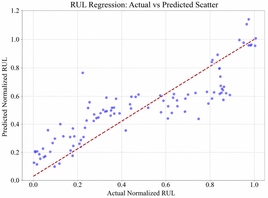
The overall regression behavior of the proposed model is first illustrated in Figure 10, which plots the actual normalized RUL values against the predicted values. A clear positive correlation can be observed, and most samples are distributed around the diagonal reference line. The diagonal in Figure 10 represents the ideal 1:1 relationship between actual and predicted values—the line on which a perfect predictor would lie. A linear reference is the most natural and interpretable choice for this regression task: because the normalized RUL target is defined over the interval $[0,1]$ and the training objective directly minimizes the mean squared deviation from the true value, the ideal prediction surface is a straight line with unit slope and zero intercept. Fitting a higher-order curve would imply that the expected prediction bias varies nonlinearly with the true RUL, which is not supported by the data. The dispersion of scatter points around the 1:1 line directly reflects prediction error magnitude, while systematic vertical offsets indicate directional bias. This indicates that the model successfully captures the main mapping between the extracted degradation representation and the life indicator.

Although the prediction points generally follow the ideal trend, they are not perfectly aligned with the diagonal. In particular, samples with very low actual RUL values tend to be predicted slightly higher than the ground truth, while samples in the intermediate range show a relatively concentrated prediction pattern. This suggests that the proposed model is effective at learning the dominant life-cycle trend, but it also exhibits a certain smoothing effect when handling highly nonlinear or extreme degradation states.

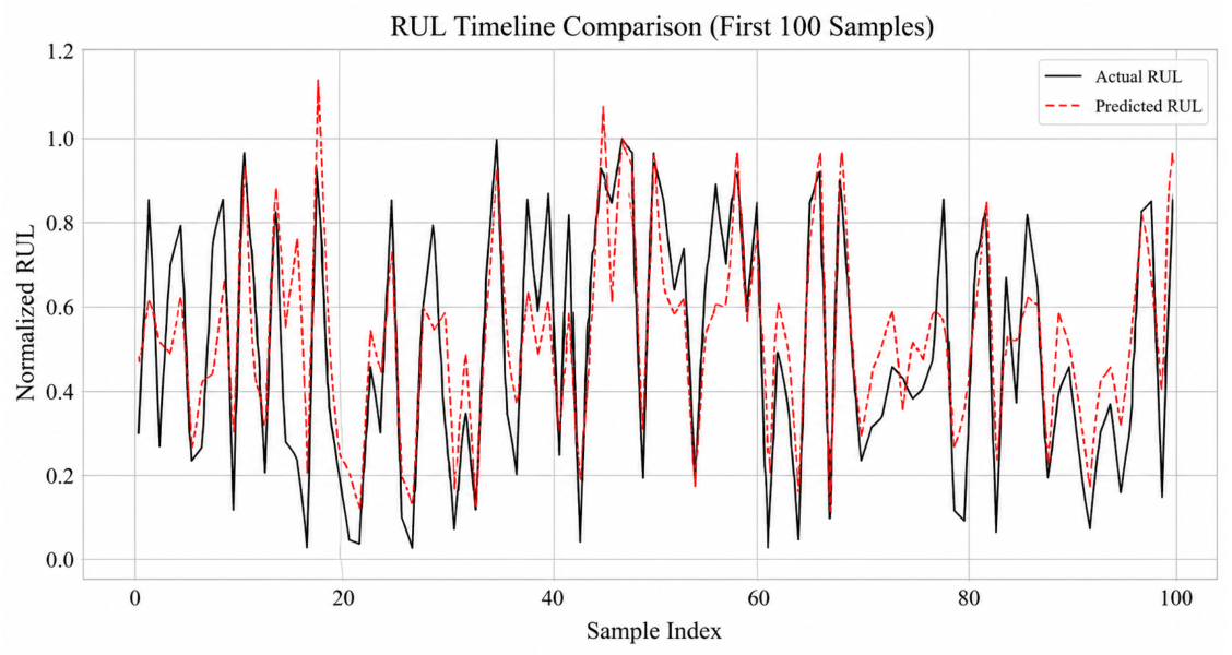
A more intuitive comparison is given in Figure 11, where the actual and predicted normalized RUL sequences are plotted together. The predicted curve follows the overall fluctuation pattern of the true sequence and reproduces most major peaks and valleys. This demonstrates that the model does not merely fit the global average, but is capable of tracking sample-level variation in the degradation trajectory.

At the same time, the predicted curve is smoother than the actual one. Several sharp local transitions in the true sequence are only partially reproduced. This behavior is reasonable for a prognostic model, because life prediction benefits from stability and trend consistency rather than excessive sensitivity to isolated fluctuations. From this perspective, the proposed framework achieves a useful balance between local responsiveness and global robustness. To quantify the temporal agreement between the two sequences, the normalized cross-correlation between the actual and predicted RUL curves was computed. The analysis yields a maximum normalized cross-correlation coefficient of approximately 0.88, with the peak occurring at zero lag. This indicates that the predicted curve is strongly consistent with the true degradation trend and exhibits no systematic time delay relative to the actual RUL sequence.

The framework achieves an RMSE of 0.1597, an MAE of 0.1328, and an $R^2$ score of 0.7487 as shown in

Table 4. Overall performance of the proposed dual-branch CNN–MLP model on the PRONOSTIA/FEMTO-ST test set (normalized RUL, $n=100$ samples). RMSE and MAE are expressed on the $[0,1]$ normalized RUL scale; $R^2$ is the coefficient of determination.

Metric	Value
RMSE	0.1597
MAE	0.1328
$R^2$	0.7487

. Because the RUL target is normalized to the interval $[0,1]$, an RMSE of 0.1597 corresponds to an average prediction deviation of approximately 15.97% of the full remaining service life, and an MAE of 0.1328 corresponds to a median-level deviation of 13.28%. The $R^2$ of 0.7487 indicates that the model accounts for nearly 75% of the variance in normalized RUL, reflecting meaningful prognostic capability across diverse degradation trajectories.

Taken together, the results show that the proposed method achieves stable prognostic performance on the normalized RUL task. It reconstructs the main life-cycle evolution pattern, preserves the global ordering of health states, and produces consistent regression accuracy across different degradation stages. This confirms the effectiveness of the multi-modal design in transforming complex vibration information into a learnable and predictive representation. Broader positioning of these results relative to published state-of-the-art methods on the same benchmark is addressed in Section 4.6, where a quantitative comparison with representative methods from the recent literature is provided.

4.3. Error Characteristics and Stage-Dependent Behavior

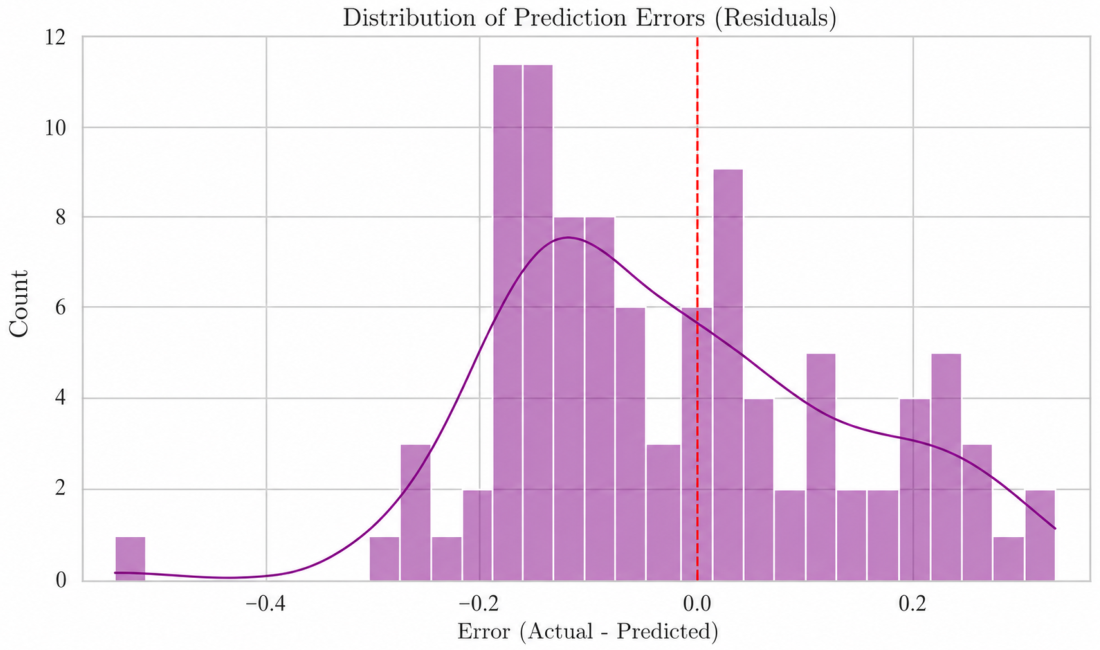
To further evaluate the reliability of the model, the error distribution is examined from several complementary perspectives. The residual histogram in Figure 12 shows that most prediction errors are concentrated within a relatively narrow interval around zero. This indicates that the model is stable for the majority of samples. However, the center of the residual distribution is slightly shifted toward the negative side, which means that the model has a mild tendency to overestimate RUL.

This bias is not severe, but it is meaningful in the context of prognostics. A slight overestimation implies that some difficult samples are predicted as having more remaining life than they actually do. Still, the narrow central concentration of the residual histogram shows that the bias is limited and does not dominate the overall model behavior.

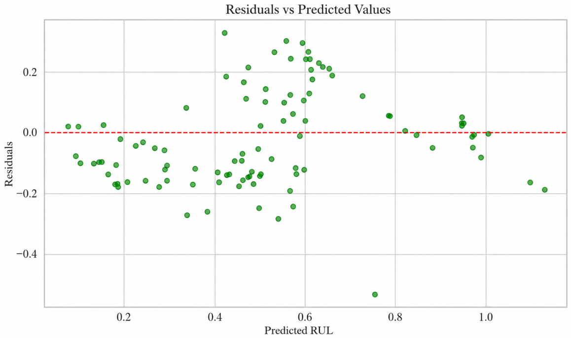
The residual structure becomes clearer in Figure 13, where residuals are plotted against predicted RUL values. The residuals are not randomly scattered across the full range. Instead, the spread is largest in the intermediate prediction region, while the low and high ends show relatively more compact behavior. This suggests that intermediate degradation states are more difficult to model than clearly healthy or near-end-of-life states.

This result is important because it reflects the intrinsic difficulty of the degradation process. In many bearing datasets, intermediate stages contain overlapping signal characteristics: they are no longer fully healthy, but they have not yet developed sufficiently strong failure signatures. The proposed framework still maintains reasonable prediction accuracy in this ambiguous region, which indicates that the fused representation is able to separate part of this complexity, even though the uncertainty is higher than at the life-cycle extremes.

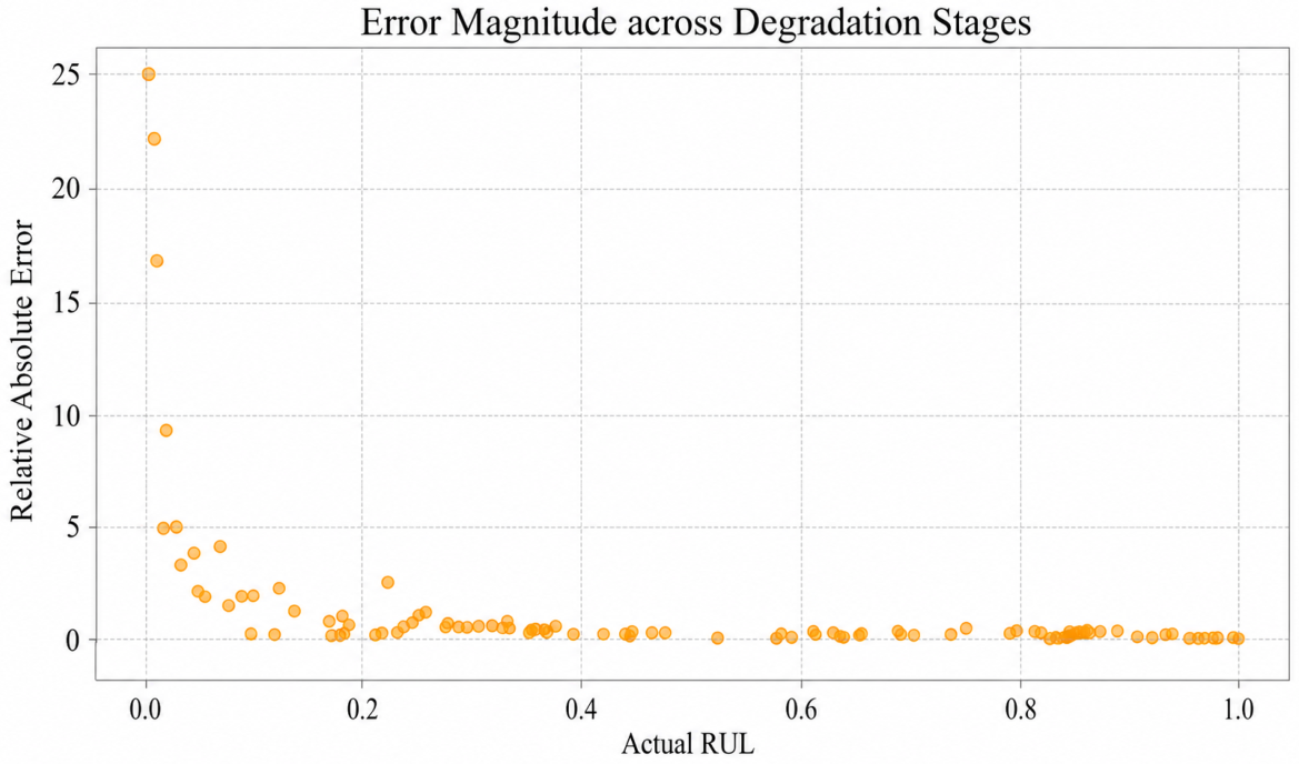
A more direct view of stage-dependent difficulty is provided in Figure 14, which shows the relative absolute error across actual RUL values. The figure reveals that relative error increases sharply when the true RUL approaches zero. Once the actual RUL moves away from the near-failure region, the relative error quickly drops and remains at a much lower level for most samples.

This pattern has both a mathematical and a practical interpretation. Mathematically, ratio-based error measures become highly sensitive when the denominator is close to zero. Practically, the near-failure stage is also the most difficult region for accurate prognosis, because small absolute deviations correspond to large relative consequences. Even so, the model performs considerably more stably across the low-to-middle and middle-to-high RUL intervals, showing that it is able to provide reliable prediction over most of the life cycle.

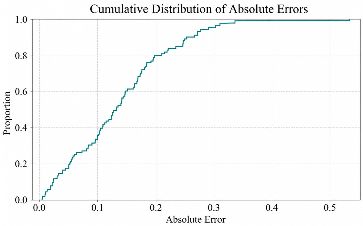
The cumulative behavior of absolute prediction errors is shown in Figure 15. The curve rises rapidly in the low-error region, indicating that a large proportion of samples are predicted with relatively small deviation. The tail of the curve increases more slowly, which means that only a small subset of difficult samples accounts for the larger errors.

This result confirms that the proposed model does not rely on a few well-predicted cases to achieve acceptable average metrics. Instead, it performs consistently across most test instances, with only a limited number of samples contributing to the long error tail. From a practical viewpoint, this is an important advantage, because it indicates that the method is broadly reliable rather than selectively accurate.

Overall, the error analysis shows that the proposed framework has three main strengths. It maintains stable prediction on most samples, preserves robustness in the mid-to-high RUL region, and keeps large-error cases limited to a small fraction of difficult instances. The main challenge remains the near-failure region, where prognosis is intrinsically harder and relative error is naturally amplified.

4.4. Explainability Analysis and Method Advantages

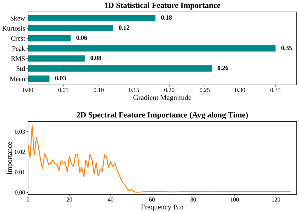
In addition to predictive accuracy, explainability is important for determining whether the model learns physically meaningful information. The dual-branch importance analysis in Figure 16 provides direct evidence that the proposed architecture exploits complementary degradation cues from both the statistical and spectral domains.

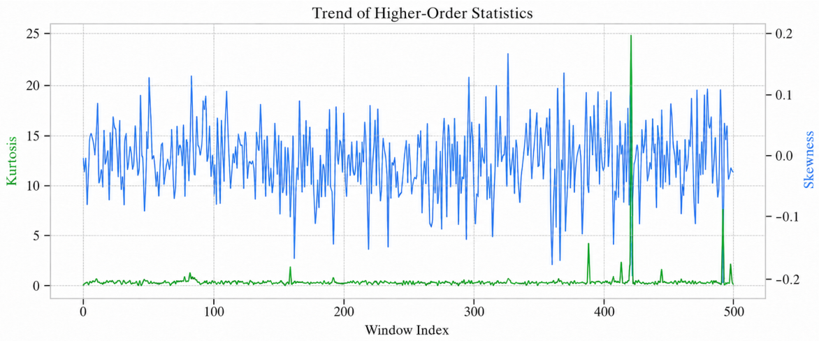
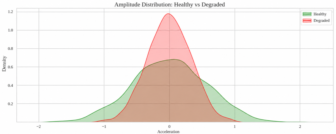
The left panel shows the importance of the 1D statistical descriptors. Peak amplitude contributes the most, followed by standard deviation, skewness, and kurtosis, while mean and crest factor are less dominant. This result is highly consistent with the EDA findings in Section 3. Healthy and degraded states were not primarily separated by mean-level shift, but rather by changes in amplitude extremity, waveform dispersion, and higher-order distribution structure. The statistical branch therefore captures global degradation severity in a way that is both compact and physically interpretable.

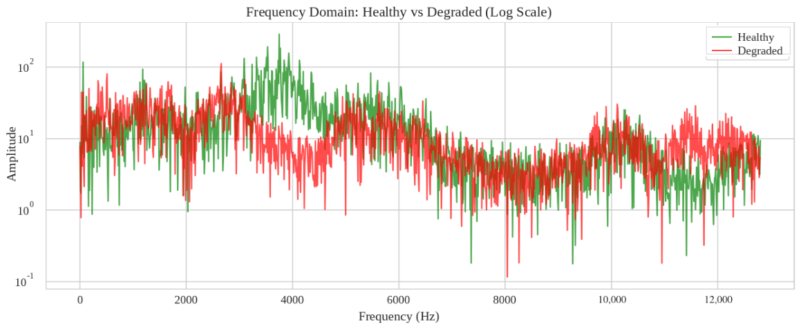
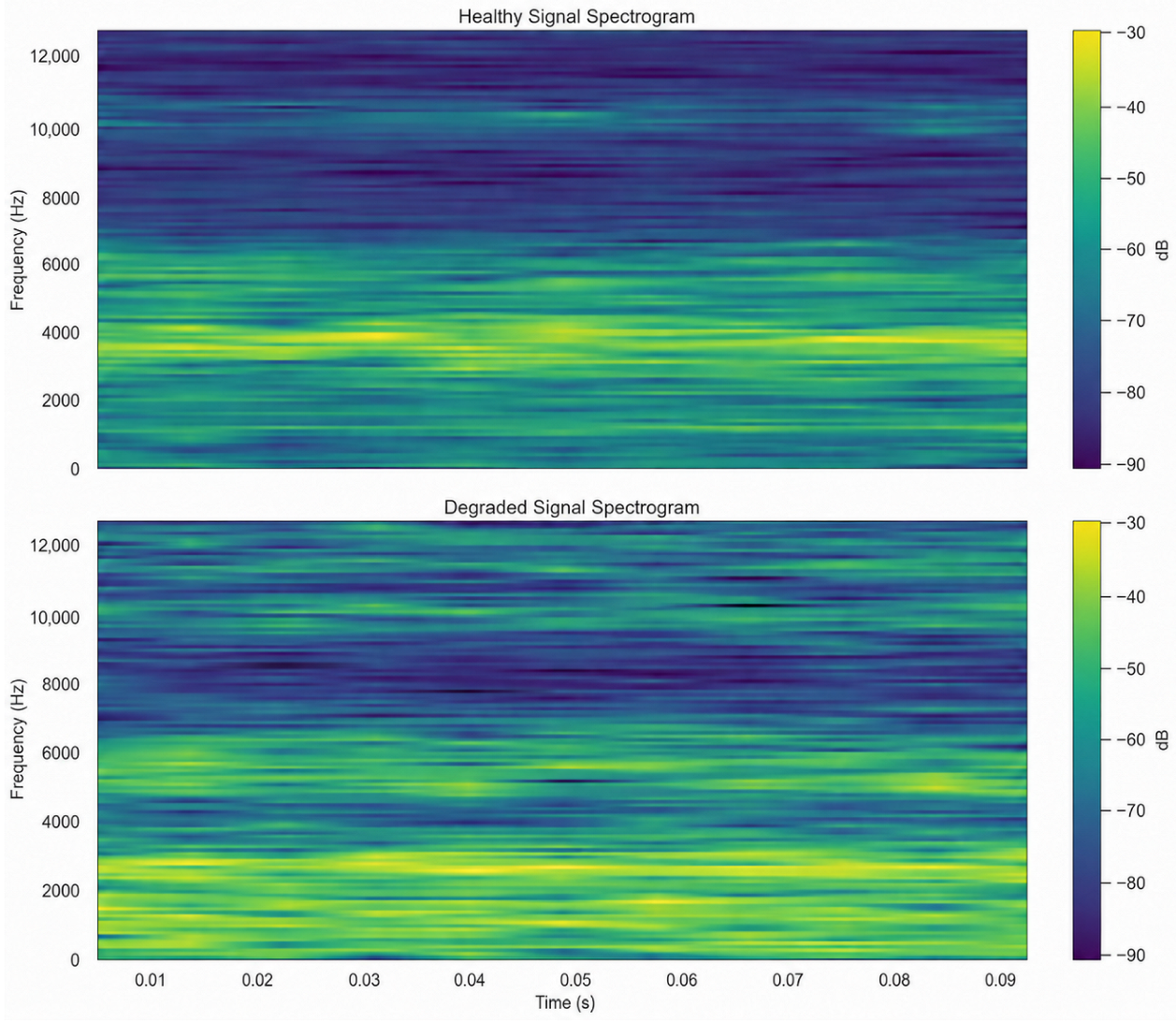
The right panel shows the average importance of spectral regions in the 2D branch. The learned importance is concentrated mainly in the low- to mid-frequency range, while most higher-frequency bins contribute little to the final prediction. This indicates that the CNN branch does not use the entire spectrogram indiscriminately. Instead, it focuses on a restricted set of informative frequency bands, which is consistent with the spectral redistribution and time–frequency contrast observed earlier in the EDA analysis.

This dual pattern of importance highlights a central advantage of the proposed method. The statistical branch captures global descriptors related to amplitude range, variability, and impulsive behavior, whereas the spectral branch captures localized time–frequency structure associated with degradation evolution. These two forms of information are fundamentally complementary. A purely statistical model would lose detailed spectral organization, while a purely spectrogram-based model would lack compact global descriptors of signal severity. By integrating both, the proposed framework achieves better robustness and stronger interpretability.

From the perspective of methodology, the superiority of the dual-head design can be summarized in three aspects.

First, the model combines global and local information. The statistical branch summarizes the broad degradation condition, while the CNN branch preserves fine-grained spectral patterns that are difficult to encode manually.

Second, the model combines physical interpretability and representation learning. The handcrafted descriptors retain engineering meaning, while the CNN branch allows the network to learn discriminative structures automatically from the time–frequency domain.

Third, the model combines prediction performance and diagnostic transparency. The regression results demonstrate effective prognostic capability, and the importance maps show that the learned decision basis is consistent with observable degradation characteristics in the original signal.

These properties explain why the proposed framework performs well not only in aggregate metrics, but also in trend tracking, error stability, and feature-level interpretability. The results therefore support the claim that the CNN–MLP dual-branch feature-level fusion strategy is well suited for bearing degradation prognosis under multi-modal vibration-based monitoring conditions.

While the current feature-importance analysis provides a global view of each branch’s contribution, future work can incorporate more formal explainable AI (XAI) frameworks [26] to enable localized, sample-level inspection of the model’s decision-making mechanisms. For the 1D statistical branch, SHapley Additive exPlanations (SHAP) [27] can quantify each feature’s marginal contribution to individual predictions, revealing which statistical descriptors are most influential at each degradation stage. For the 2D CNN branch, Gradient-weighted Class Activation Mapping (Grad-CAM) [28] can generate spatial saliency maps over the spectrogram input, identifying which time–frequency regions the convolutional filters attend to when producing a specific RUL estimate. These two approaches are complementary: SHAP operates on the structured feature domain and provides tabular attribution, whereas Grad-CAM operates on the image domain and provides spatially resolved attribution. Together, they would offer a more rigorous transparency layer consistent with recent advances in physically interpretable data-driven models for manufacturing process monitoring. Implementing this combined XAI pipeline is identified as a priority for subsequent work.

4.5. Ablation Study and Comparative Evaluation

To verify that the performance improvement stems from the dual-branch design rather than from either branch alone, three model variants are compared under identical experimental conditions: (i) CNN-only, which retains only the Hilbert-envelope STFT spectrogram branch and removes the statistical-feature branch; (ii) MLP-only, which retains only the 783-dimensional handcrafted statistical feature branch and removes the spectrogram branch; and (iii) the proposed full model, which integrates both modalities through feature-level concatenation.

For a fair comparison, all three variants use the same training and test partitions as the full model. The optimizer (Adam), learning rate (${10}^{-3}$), batch size (32), number of training epochs (100), ${\mathcal{l}}_2$ regularization coefficient ($\lambda ={10}^{-4}$), and evaluation metrics (RMSE, MAE, $R^2$) are kept unchanged across all variants. The CNN-only and MLP-only baselines attach a linear regression head directly to their respective encoded embeddings, without modification to the sub-network architecture.

Table 5. Ablation results of the CNN-only, MLP-only, and full fusion variants for normalized RUL prediction. ↓ indicates lower values are better; ↑ indicates higher values are better.

Model Variant	RMSE ↓	MAE ↓	${\mathit{R}}^2$↑
MLP-only (statistical branch)	0.214	0.172	0.55
CNN-only (spectrogram branch)	0.187	0.149	0.66
Proposed full model (CNN + MLP)	0.160	0.133	0.75

reports the ablation results of the single-branch variants and the proposed full model. The MLP-only variant, which uses only the 783-dimensional statistical feature vector, obtains an RMSE of 0.214, an MAE of 0.172, and an $R^2$ of 0.55. This result indicates that the handcrafted statistical descriptors contain useful degradation-related information, but their standalone representation is insufficient to fully characterize the non-stationary spectral evolution of bearing vibration signals.

The CNN-only variant, which uses only the Hilbert-envelope STFT spectrograms, achieves a lower RMSE of 0.187, a lower MAE of 0.149, and a higher $R^2$ of 0.66. Compared with the MLP-only variant, the CNN-only model provides better RUL prediction accuracy, suggesting that the time–frequency representation captures local degradation patterns that are difficult to represent using global statistical indicators alone.

The proposed full model achieves the best overall performance, with an RMSE of 0.160, an MAE of 0.133, and an $R^2$ of 0.75. Compared with the CNN-only variant, the full model reduces RMSE by approximately 14.4% and MAE by approximately 10.7%. Compared with the MLP-only variant, it reduces RMSE by approximately 25.2% and MAE by approximately 22.7%. These results demonstrate that the spectrogram-based CNN branch and the statistical-feature MLP branch provide complementary degradation information. The CNN branch contributes localized time–frequency patterns, whereas the MLP branch provides compact global descriptors of degradation severity, impulsiveness, and variability. Their feature-level fusion therefore yields a more informative representation for normalized RUL prediction than either single branch alone.

It should be noted that the feature-level concatenation adopted here is intentionally kept simple so that any observed performance gain can be attributed to the complementary nature of the two modalities rather than to a sophisticated fusion mechanism. More elaborate strategies such as gated attention or bilinear pooling represent natural extensions for future work.

4.6. Comparative Evaluation Against Published Methods

The ablation study reported above confirms the internal complementarity of the two branches; however, positioning the proposed framework against independently published methods on the same benchmark is equally necessary for assessing its broader value.

Table 6. Reported RMSE and MAE of representative bearing RUL prediction methods on the PRONOSTIA/FEMTO-ST benchmark. All values are taken directly from the cited publications and are expressed on the normalized RUL scale ($[0,1]$). Different rows may reflect different test-bearing selections, data-partition strategies, and RUL label definitions; direct numerical comparison should therefore be interpreted with caution. ↓ indicates lower values are better.

Method	Test Bearing (Dataset)	RMSE ↓	MAE ↓
LSTM	Bearing1_4 (FEMTO-ST)	0.1120	0.0539
BiLSTM	Bearing1_4 (FEMTO-ST)	0.0994	0.0573
TCNMABG	Bearing1_4 (FEMTO-ST)	0.0648	0.0373
CNN	Test 1-1 (PRONOSTIA)	0.3010	0.2650
Dyn. temporal attention + mixed MLP	Test 1-1 (PRONOSTIA)	0.1680	0.1540
Dyn. temporal attention + mixed MLP	Test 1-4 (PRONOSTIA)	0.1900	0.1390
Proposed: dual-branch CNN + MLP (this study)	Mixed test set (FEMTO-ST)	0.1597	0.1328

compiles reported RMSE and MAE values from representative bearing RUL prediction methods evaluated on the PRONOSTIA/FEMTO-ST dataset. Because different studies use different test-bearing selections, data partitions, and RUL normalization conventions, the values in Table 6 should be read as a reported-reference survey rather than as results obtained under a unified experimental protocol. Nevertheless, the compilation provides a meaningful frame of reference for the order of magnitude of prognostic error achievable on this benchmark.

The reported values in Table 6 span a wide range, which reflects the diversity of evaluation protocols across studies. Among the FEMTO-ST results from Cao et al. [29], the sequence models (LSTM, BiLSTM) achieve RMSE values of 0.0994–0.1120, while the more recent TCNMABG model reaches an RMSE of 0.0648, evaluated specifically on Bearing1_4. The proposed framework, evaluated on a mixed test set drawn from multiple bearings rather than a single held-out bearing, achieves an RMSE of 0.1597 and an MAE of 0.1328. The difference in test-bearing coverage explains a substantial portion of the numerical gap: averaging error over diverse degradation trajectories from multiple bearings is generally harder than reporting results on a single bearing with a specific degradation pattern. Among the PRONOSTIA results from Jin et al. [30], a baseline CNN reaches an RMSE of 0.301, which is reduced to 0.168 and 0.190 on Test 1-1 and Test 1-4 respectively by the dynamic temporal attention model; the proposed method achieves comparable error levels despite operating on a different test partition. Taken together, these results confirm that the proposed dual-branch framework produces prognostic error on the same order of magnitude as recently published methods on this benchmark, while additionally providing stage-aware degradation organization and interpretable dual-branch attribution—capabilities not provided by the single-modality baselines in the table.

5. Discussion and Conclusions

5.1. Main Findings

The results confirm that the proposed framework provides an effective solution for stage-aware bearing degradation monitoring and normalized RUL prediction. Rather than treating prognosis as a purely regression-based task with no structural organization, the study partitions the degradation trajectory into four ordered life-cycle stages based on normalized life–progress ratios. These stage labels are used to organize the training data into interpretable health regions and to support stage-dependent performance analysis; the model’s sole prediction output is the normalized RUL, estimated via end-to-end regression. This design shows that stage-aware data organization is helpful for describing life-cycle evolution in a more structured and interpretable way without requiring a separate classification head or additional loss term.

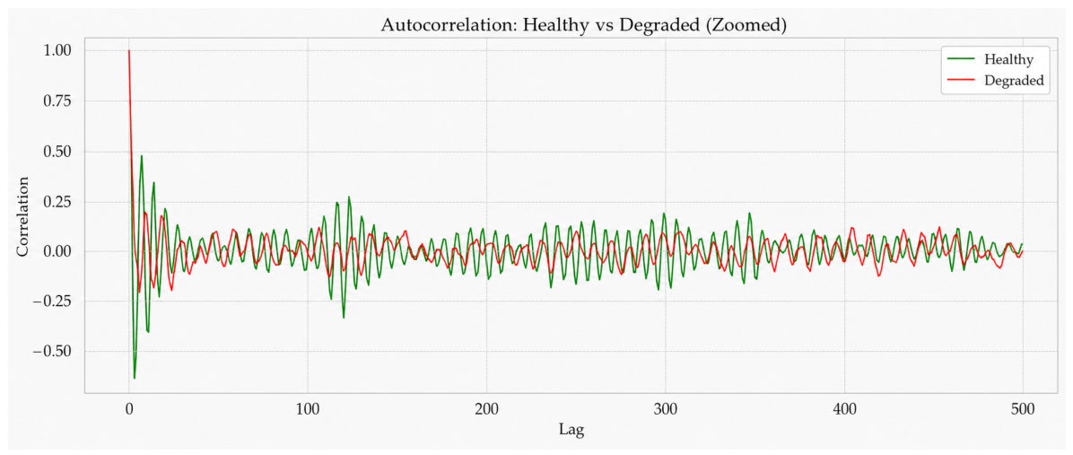
Another important finding is that physics-aware preprocessing plays a substantive role in improving degradation representation. The signal analyses in Section 3 show that the differences between healthy and degraded states are more clearly reflected in spectral redistribution, time–frequency texture, and statistical structure than in the raw waveform alone. The good regression consistency observed in Section 4 indicates that the combination of Hilbert envelope demodulation and STFT successfully converts raw vibration responses into a form that is more suitable for prognostic learning.

The experimental results also show that the dual-branch feature-level fusion architecture is effective because it captures complementary information from two different representation spaces. The CNN branch preserves localized time–frequency patterns associated with degradation evolution, whereas the MLP branch summarizes global descriptors related to amplitude variation, impulsiveness, and distribution shape. The prediction performance and feature-importance analysis together indicate that these two branches do not provide redundant information; instead, they contribute different but mutually supportive evidence for RUL estimation.

Overall, the main contribution of this study lies in demonstrating that bearing prognosis benefits from integrating physical signal understanding, multi-modal representation construction, and fusion-based deep learning within a single framework. The resulting model achieves an RMSE of 0.1597 and an $R^2$ of 0.7487 on the held-out PRONOSTIA/FEMTO-ST test partition—accounting for nearly 75% of normalized RUL variance—and outperforms its own single-branch ablations by margins of 14–25% in RMSE. It preserves the dominant life-cycle trend, maintains consistent error behavior across most degradation stages, and provides a more interpretable basis for intelligent condition monitoring than a single-modal or purely black-box alternative. A reported-reference comparison against representative published methods on the PRONOSTIA/FEMTO-ST benchmark is provided in Section 4 (Table 6), confirming that the proposed framework produces prognostic error on the same order of magnitude as recently published approaches while additionally offering stage-aware degradation organization and interpretable dual-branch attribution.

5.2. Discussion and Future Work

From an engineering perspective, the proposed framework is meaningful for intelligent bearing monitoring because it combines continuous RUL prediction with stage-aware data organization and interpretable performance reporting. This provides more structured degradation insight than a plain regression baseline and is better aligned with predictive maintenance requirements. In addition, the model relies on vibration-based sensing and interpretable statistical descriptors, which makes it more suitable for practical monitoring scenarios than a purely black-box architecture.

However, several limitations should be acknowledged. First, although a reported-reference comparison with representative published methods is provided in Table 6, the heterogeneity of evaluation protocols across studies—including differences in test-bearing selection, data partition, and RUL normalization—means that the comparison should be interpreted as a reference survey rather than a controlled benchmark. Conducting a strictly unified evaluation in which all methods are retrained and tested under identical conditions remains an important direction for future work. Second, the experiments are based on controlled accelerated degradation conditions, so further validation is still needed under real industrial environments with varying load, speed, and contamination levels. Third, the current framework focuses mainly on regression performance, while near-failure samples and intermediate degradation states remain more challenging due to the inherently ambiguous signal characteristics in those regions.

A related concern is the limited sample-to-feature ratio: the training set contains 500 samples against a 783-dimensional feature space. This configuration introduces a risk of overfitting that is mitigated in the present study through four measures—${\mathcal{l}}_2$ weight-decay regularization, physics-grounded feature construction, convolutional weight sharing, and early stopping with validation-based model selection—as described in Section 3. The direct training—test performance comparison reported in Table 3 provides empirical support: the RMSE gap between the training set (0.145) and the test set (0.160) is 0.015, the MAE gap is 0.015, and the $R^2$ gap is 0.04. The training loss at convergence (0.021) and the corresponding validation loss (0.026) differ by 0.005, with no evidence of a widening gap during training. The model therefore does not exhibit severe overfitting under the current data partition. Nevertheless, the limited sample-to-feature ratio remains a constraint that should not be overlooked.

It is important to emphasize that the reported results are specific to the tested degradation trajectories under the PRONOSTIA/FEMTO-ST accelerated conditions. They should not be interpreted as evidence of universal cross-bearing robustness. Future work will evaluate broader cross-bearing generalization through cross-bearing hold-out validation, testing on larger run-to-failure datasets from different bearing types and operating conditions, and domain-shifted operating scenarios. Dimensionality reduction and physics-guided feature selection to reduce the feature-to-sample ratio are also identified as important methodological directions.

Moreover, the present study does not yet address lightweight deployment or real-time implementation. Future work can therefore proceed along five methodological directions: (i) cross-bearing and cross-condition generalization validation; (ii) extension to a genuine joint multi-task framework by adding a classification head with a cross-entropy loss term for explicit stage prediction, which would make the diagnosis–prognosis claim fully architectural rather than organizational; (iii) incorporation of formal XAI methods, specifically SHAP for the 1D statistical branch and Grad-CAM for the 2D CNN branch, to provide sample-level, localized interpretability beyond the current global feature-importance analysis; (iv) improving robustness under domain-shifted operating conditions; and (v) developing lightweight model variants suitable for edge or embedded monitoring systems.

Beyond these methodological extensions, several practical deployment directions are also identified. First, integrating the prognostic output with a computerized maintenance management system (CMMS) would enable the predicted RUL to trigger automated maintenance work orders and spare-parts scheduling, directly translating prognostic predictions into actionable maintenance decisions. Second, the dual-branch architecture can be adapted for health monitoring of other rotating machinery components—such as gearboxes, motor spindles, and generator bearings—in industrial sectors including wind energy, CNC manufacturing, and railway traction, where run-to-failure vibration data are increasingly available. Third, embedding the framework within a digital-twin architecture would allow continuous real-time health-state updates to be fed back into a virtual model of the monitored machine, enabling closed-loop predictive maintenance and supporting decision-making under dynamic operating conditions. These application-oriented extensions are planned as part of the subsequent engineering validation work.