1. Introduction
As both the global energy transition and applications of the dual-carbon strategy advance, flexible DC transmission (also known as high-voltage DC (HVDC) transmission) based on modular multilevel converters (MMCs) has emerged as a key technology for next-generation power systems owing to its high control flexibility, excellent performance upon grid integration, and reliability under high power supplies [
1,
2,
3]. However, flexible DC grids exhibit notable low-damping characteristics. Once a fault occurs on a DC transmission line, the submodule capacitors in the converter station rapidly discharge toward the fault point, resulting in a sharp increase in fault current. This has led to stringent requirements for the operating speed and sensitivity of relay protection mechanisms [
4].
Existing single-ended protection schemes primarily employ voltage traveling wave (TW) derivatives and polar wave derivatives as protection schemes. These schemes do not require communication between the two ends, exhibit a fast operating speed, and thus have been widely applied in practical projects [
5]. However, when these single-ended TW protection schemes encounter high-resistance faults or remote-end faults, severe attenuation of the fault-generated TWs and interference from the subsequent refracted and reflected TWs lead to reduced identification sensitivity and protection “dead zones” [
6]. To address these issues, researchers have proposed various additional single-ended protection schemes.
According to the differences among their fault feature extraction methods, existing single-ended protection schemes can be classified into three categories: time-domain methods, frequency-domain methods, and methods based on the overall waveform characteristics. For time-domain methods, protection schemes are constructed based on the time-domain features extracted after faults occur on DC transmission lines. In references [
7,
8], protection criteria were established on the basis of the voltage change rate and the transient voltage ratio across the current-limiting reactor, improving the tolerance of the scheme to fault resistance. Moreover, in references [
9,
10], protection schemes based on the rate of voltage change in the current-limiting reactor and the arrival time of the first peak were proposed, which allow for rapid fault identification. However, when the current-limiting reactor is small, differences in the fault characteristics become insignificant, and the sensitivity is easily affected by line boundary effects. In reference [
11], a protection scheme based on modal quantities was analyzed; in this scheme, the line-mode current-limiting reactor voltage was used to identify internal and external faults. This scheme is easy to implement and exhibits a strong anti-noise capability; however, its sensitivity under high-resistance faults requires improvement. These studies show that existing single-ended protection schemes based on time-domain characteristics are still affected by the refraction and reflection of TWs under remote high-resistance faults.
For frequency-domain methods, protection schemes are constructed by using time–frequency-domain extraction tools to obtain characteristic quantities at specific frequencies. In references [
12,
13], the fast Fourier transform (FFT) and short-time Fourier transform (STFT) were employed, respectively, to extract characteristic quantities at corresponding frequencies for fault type discrimination. However, both these schemes are highly affected by the time window and are susceptible to noise interference. In references [
14,
15], wavelet transforms were used to extract high-frequency voltage components for fault type discrimination, but their adaptability under weak boundary requires further improvement, and in references [
16,
17], protection schemes were constructed using electrical quantities from multiple characteristic frequency bands. However, the computational principles of these methods are relatively complex. These studies show that frequency-domain-based single-ended protection schemes suffer from strong noise interference and high computational burden.
In contrast, protection schemes based on the overall waveform characteristics mainly rely on the overall evolution of the fault-generated TWs during propagation. In reference [
18], the fault section was identified by analyzing the polarity characteristics of the refracted and reflected TWs along the transmission line, demonstrating certain adaptability under weak boundaries. In reference [
19], a protection criterion based on the similarity between the measured and reference-voltage waveforms was proposed, and in reference [
20], the measured fault-generated TWs were fitted using the reverse TW as the reference waveform under internal faults. However, under these conditions, the modulus maxima of the wavelet transform must be used to determine the arrival times of the initial and subsequent TWs, and under near-end or far-end faults, the protection scheme is affected by multiple TW refractions and reflections. In references [
21,
22], the expression of the reverse TWs under external faults was used as the reference function to fit fault-generated TWs; however, these algorithms are prone to overfitting when applied to low-resistance conditions.
Existing methods based on the overall waveform characteristics are affected by TW refraction and reflection. Moreover, under low-fault-resistance conditions, both internal and external fault-generated TWs attenuate rapidly, and traditional nonlinear fitting algorithms are prone to overfitting. Even when external faults exhibit double-exponential characteristics, traditional algorithms can still obtain small residuals when the fitting is performed using a single-exponential model. This makes it difficult to distinguish between internal and external faults under low-resistance conditions, and thus improvements are needed to increase the reliability of fault identification. To address the overfitting tendency of traditional nonlinear fitting algorithms, in this paper, a single-ended protection scheme for flexible DC transmission lines based on the residuals of the composite fit of the fault-generated reverse TW is proposed. Specifically, protection criteria are proposed based on the differences in the waveform structure characteristics of the reverse TWs under internal and external faults. The main contributions of this study are as follows:
(1) Based on the flexible DC grid fault equivalent model, analytical expressions of reverse TWs under internal and external faults are derived, revealing an essential difference in theoretical waveform structures: internal faults exhibit single-exponential attenuation characteristics, whereas forward external faults exhibit double-exponential attenuation characteristics. This provides a reference for analyzing fault waveform characteristics.
(2) To suppress the adverse effects of refracted and reflected TWs on the waveform characteristics, an adaptive constant-value flattening method for waveform preprocessing is proposed. A tolerance band is established based on the extreme points of the initial TW, effectively preserving its exponential attenuation characteristics while addressing the issue that the refraction and reflection of the TWs distort the subsequent waveform structure and thus affect fault detection.
(3) A composite fitting strategy combining the Levenberg–Marquardt (LM) nonlinear optimization algorithm and the Moore–Penrose pseudoinverse (PINV) linear least-squares algorithm is proposed. In this strategy, the composite fitting residuals are utilized to fundamentally overcome the drawback of traditional algorithms in that they are prone to overfitting under low-resistance faults. In this way, the residual differences between internal and external faults are emphasized and the reliability of the protection scheme is increased.
2. Analysis of the Characteristics of Reverse Traveling Waves for Line-Mode Voltage
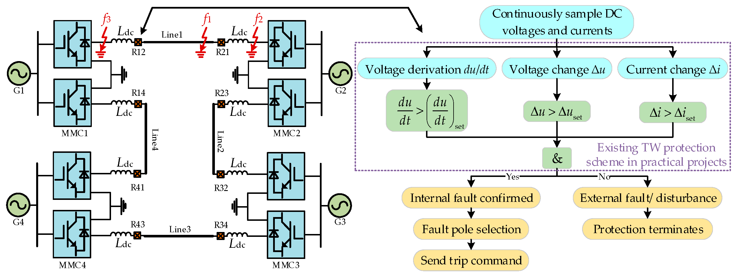
Figure 1 shows the topology of a typical four-terminal flexible DC grid, in which four modular multilevel converter (MMC) stations are interconnected through four DC transmission lines to form a ring network. To suppress the rising fault current rate, current-limiting reactors
Ldc are installed at both ends of each line; R12–R43 represent the protection measurement points at both ends of each line. In the following theoretical analysis, line 1 and its left-side protection measurement point R12 are taken as the study objects. An internal positive-pole-to-ground fault (PGF)
f1 occurs within line 1 and an external fault
f2 occurs on the remote current-limiting reactor side of the line.
The four-terminal flexible DC grid model studied in this paper is built with reference to the Zhangbei ±500 kV four-terminal flexible DC grid project in China. The conventional single-ended traveling wave (TW) protection scheme widely used in such projects relies on voltage derivation, current change, and voltage change criteria. However, it suffers from insufficient sensitivity under remote faults and high-resistance faults, where the TW amplitude is severely attenuated and the protection may fail to operate. A new protection scheme is therefore needed to address these issues.
2.1. Fault Equivalent Model of the Flexible DC Grid
To eliminate the interference of pole-to-pole coupling in the analysis of the fault-generated TWs, the phase-mode transformation is adopted to decouple the voltage and current quantities in the phase domain into mutually independent line-mode and zero-mode components. The transformation matrix is expressed as follows:
where
up and
un denote the positive and negative pole voltages, respectively;
ip and
in denote the positive and negative pole currents, respectively;
u0 and
u1 represent the decoupled zero-mode and line-mode voltage components, respectively; and
i0 and
i1 represent the decoupled zero-mode and line-mode current components, respectively.
During the propagation of transient TWs along the line, the zero-mode component is significantly affected by the ground’s frequency-dependent parameters, resulting in severe attenuation and waveform distortion. In contrast, the line-mode component propagates between the two pole conductors and is less affected by frequency and dispersion effects; thus, it exhibits a stable wave velocity and low waveform distortion. Therefore, in this study, we primarily focus on the line-mode component for extracting the fault waveform characteristics.
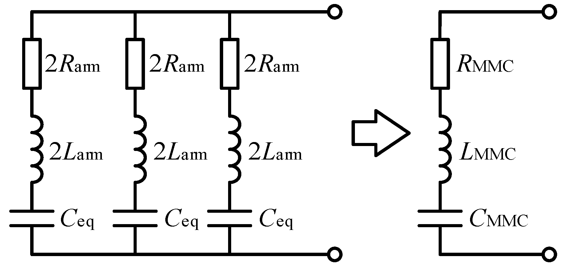
During the initial TW stage after a fault occurs, the MMC station can be represented by an RLC series model [
23]. The MMC generally consists of three phases and six bridge arms, where each bridge arm comprises
N submodules connected in series with a bridge arm reactor
Larm. Based on the principle of equivalent capacitor energy storage, the single-phase equivalent capacitance
Ceq can be expressed as 2
Csm/
N. Accordingly, the MMC can be equivalently represented as a second-order RLC series circuit, with its equivalent parameters defined as follows:
where
Req,
Leq, and
Ceq denote the single-phase equivalent resistance, equivalent inductance, and equivalent capacitance of the MMC, respectively. The corresponding equivalent circuit is shown in
Figure 2.
Moreover, the DC transmission line is modeled using the frequency-dependent Bergeron model, in which the propagation function is employed to describe the delay, attenuation, and distortion processes of the TWs along the line. Based on the general frequency-domain solution for TW propagation along the line established in the existing reference, the boundary conditions at both ends of the line (
x = 0 and
x =
L) are substituted to solve for the unknown coefficients. After mathematical rearrangement, the fundamental equations of the Bergeron model incorporating the distributed parameter characteristics of the DC line can be obtained as follows [
23]:
where
Um1(
t) and
Un1(
t) denote the line-mode voltages at terminal M and N of the line, respectively;
Im1(
t) and
In1(
t) denote the line-mode currents at terminal M and N, respectively;
Zc1 is the line-mode wave impedance;
γ1 represents the line-mode propagation constant of the DC line; and
τ is the traveling wave propagation time along the line.
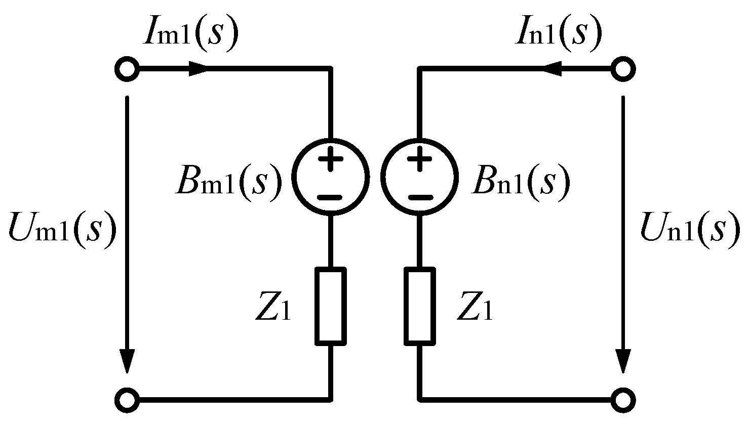
Bm1(
t) and
Bn1(
t) are the Bergeron equivalent current sources, the physical meaning of which is the equivalent current injected into the local terminal at the present instant, influenced by the historical traveling waves generated by the earlier voltage and current at the opposite terminal
τ. Based on Equation (3), a line-mode Bergeron equivalent circuit model of the transmission line can be established, as shown in
Figure 3.
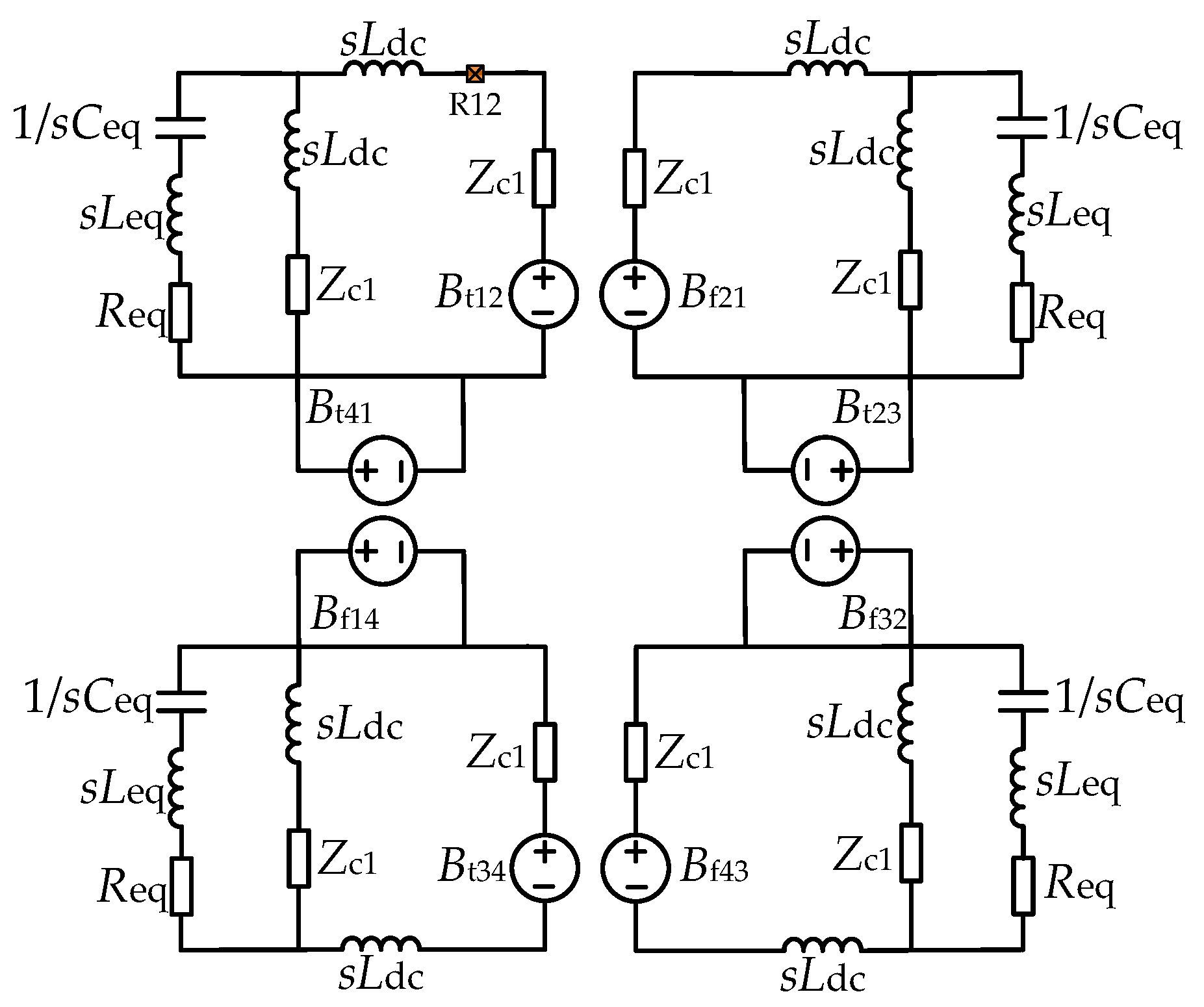
Based on the above simplified equivalent models of the MMC station and DC transmission line, the equivalent line-mode component model of the flexible DC grid can be derived, as shown in
Figure 4. The equivalent voltage sources
Bt12–
Bf14 in the figure reflect the attenuation characteristics of the TWs during their propagation along the DC transmission line. On the basis of
Figure 4, the time-domain expressions and characteristics of the reverse TWs of the line-mode voltage under internal and external faults on the DC transmission line can be analyzed in detail.
2.2. Analysis of the Reverse Traveling Waves of the Line-Mode Fault Voltage Under Internal Faults
For internal faults, it is assumed that a PGF occurs at a distance of
x away from protection measurement point R12, with a fault resistance of
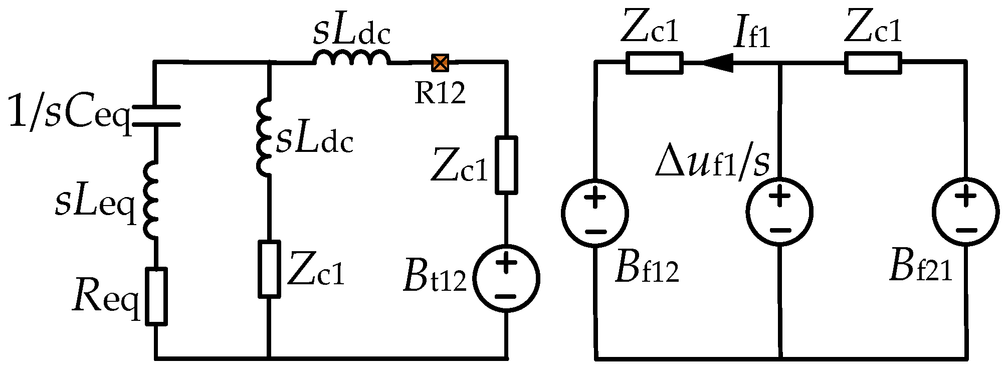
Rf. The fault point divides line 1 into two sections. According to the fault superposition principle, this fault can be equivalently represented by an additional voltage source. Before the TW of the initial fault reaches the remote converter station and is reflected, the Bergeron equivalent voltage sources of the adjacent lines are zero. By combining the characteristics of the initial fault TW with those of the equivalent circuit model, an equivalent circuit of the additional line-mode fault component for internal fault
f1 can be obtained, as shown in
Figure 5.
At this time, the line-mode voltage fault component Δ
uf1 at the fault point can be expressed as follows:
where
Zc1 and
Zc0 are the line-mode and zero-mode surge impedances of the transmission line, respectively, and
Uf is the steady-state DC voltage before the fault occurs.
For a uniform transmission line, the reverse TW of the line-mode voltage can be obtained from the voltage and current at the measurement point as follows:
Considering the attenuation and dispersion characteristics of the transmission line, the reverse TW of the line-mode fault voltage for an internal fault at the protection measurement point can be expressed in the complex frequency domain as follows:
where
e−sT is the pure time delay (with
T =
x/
v) generated by a TW propagating at velocity
v over a distance
x along the line;
ka1 is the line-mode attenuation coefficient per unit length of the DC transmission line; and
τa1 is the line-mode dispersion time constant per unit length of the DC transmission line.
By performing an inverse Laplace transform on both sides of Equation (4), an analytical expression of the reverse TW of the fault voltage for an internal fault in the time domain can be obtained as follows:
For convenience in the characteristic analysis, this expression is simplified into the following standard algebraic form:
The coefficients of the constant terms are as follows:
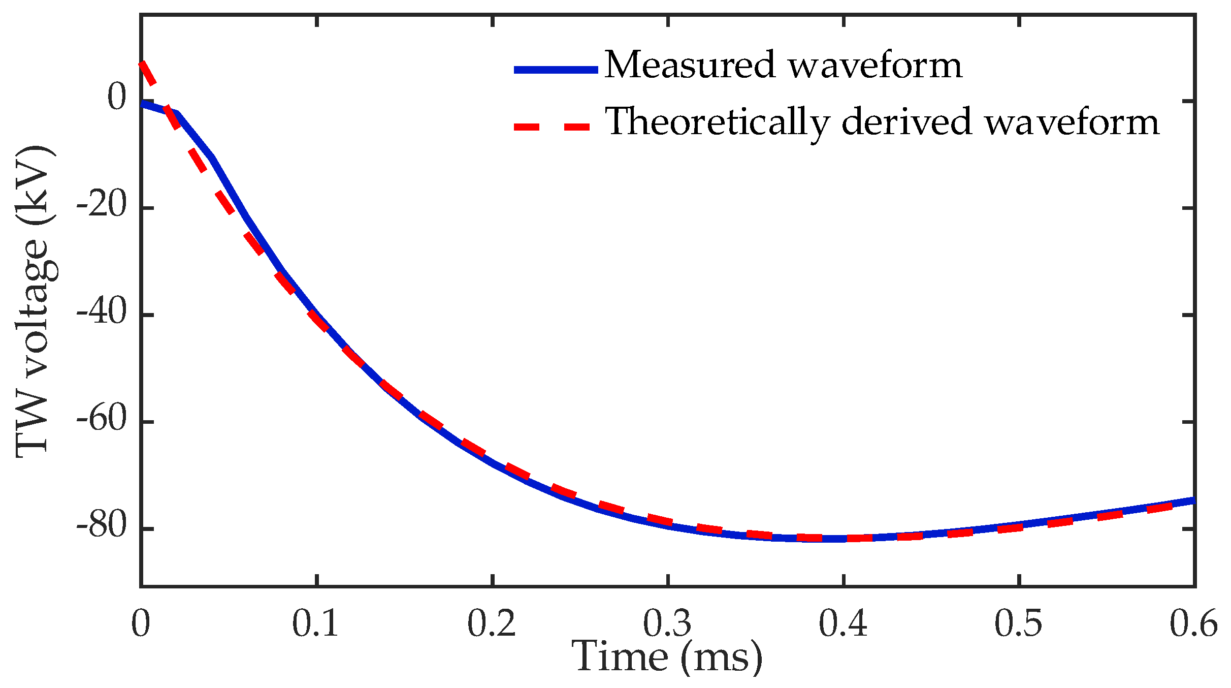
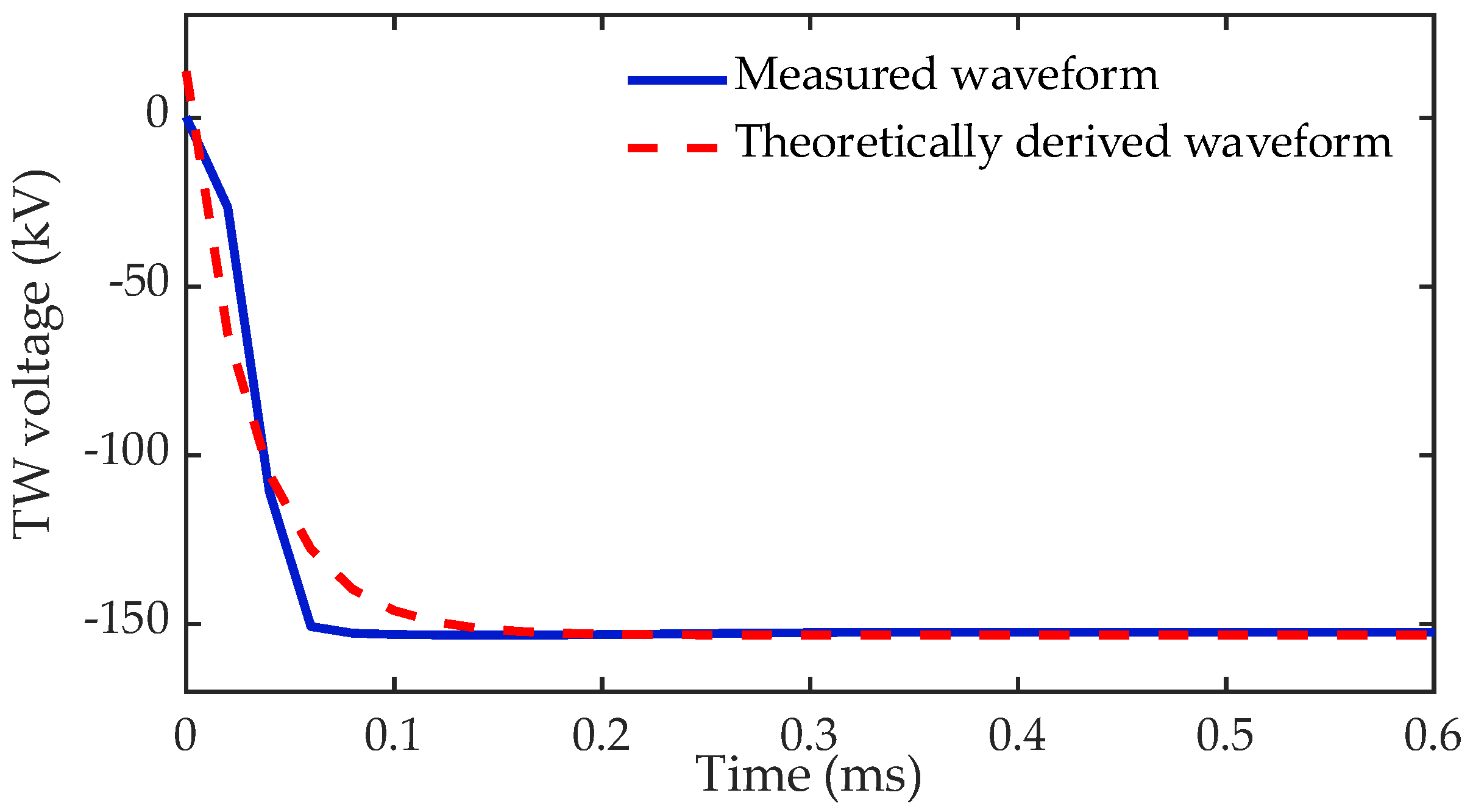
The above derivation reveals that when an internal fault occurs and the subsequent refracted and reflected waves are neglected, the time-domain expression of the reverse TW of the line-mode fault voltage consists of a single-exponential attenuation function and a constant term, with the specific waveform shown in
Figure 6. The fault resistance
Rf exists only in Δ
uf1, indicating that it only affects the amplitude of the single-exponential waveform and does not alter the structural characteristics of its attenuation trajectory.
The small deviation between the measured and theoretically derived waveforms arises from approximating the frequency-dependent line model as a first-order inertial system governed by the per-unit-length attenuation coefficient and dispersion time constant. Although this approximation introduces minor errors, it adequately captures the frequency-dependent propagation characteristics of the transmission line and yields a tractable analytical expression for the fault reverse TW.
2.3. Analysis of the Reverse Traveling Waves of the Line-Mode Voltage Under External Faults
In the case of the external fault model, its main difference from the internal fault model is that the initial transient TW generated by fault point
f2 is inherently limited by the current-limiting reactor
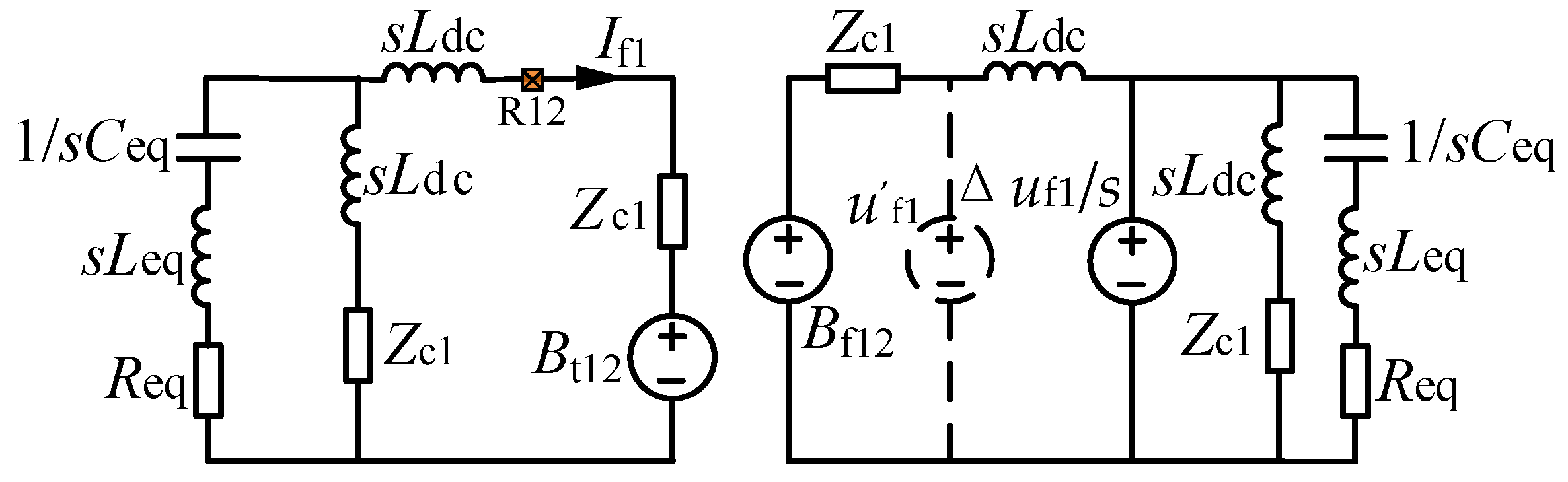
Ldc before propagating through DC line 1 and reaching protection measurement point R12. Before the ensuing refracted and reflected waves arrive, the Bergeron equivalent voltage source of the adjacent lines is zero. Considering the equivalent impedance of the current-limiting reactor and its boundary constraint effect, an equivalent circuit of the fault-induced additional line-mode component at measurement point R12 under external fault
f2 can be established, as shown in
Figure 7.
Considering the boundary condition introduced by the equivalent impedance
sLdc of the current-limiting reactor, the complex frequency-domain expression of the line-mode voltage reverse TW under external faults at the protection measurement point becomes:
where
L is the total length of the DC transmission line.
To obtain a time-domain expression, Equation (10) can be decomposed considering algebraic theory and the partial fraction expansion method, and after applying the inverse Laplace transform, a time-domain analytical expression for external faults is obtained:
The coefficients of the constant terms are given as follows:
The above derivation reveals that introducing the boundary current-limiting reactor
Ldc introduces an additional pole in the denominator of the frequency-domain expression, resulting in a time-domain transformation. Under external faults, the expression of the reverse TW of the line-mode voltage at the measurement point contains the superposition of two exponential attenuation terms and a constant term. The detailed waveform is shown in
Figure 8. The first exponential term is governed by line dispersion
τa1 and the second is governed by the time constant
Ldc/
Zc1 of the current-limiting reactor.
2.4. Difference in Waveform Characteristics Under Internal and External Faults
A comparison of the mathematical analyses in
Section 2.2 and
Section 2.3 reveals the essential differences in the time-domain expressions of the reverse TWs of the line-mode voltage under internal and external faults. In terms of the waveform structure, the internal fault waveform exhibits single-exponential attenuation characteristics, and its time-domain analytical expression consists of a constant term and a single-exponential attenuation term controlled by line dispersion. For forward external faults, the time-domain analytical expression is the superposition of two exponential attenuation terms and a constant term, exhibiting double-exponential attenuation characteristics. Under the influence of fault resistance, the single-exponential attenuation trajectory of internal faults exhibits a certain degree of stability. The theoretical derivation reveals that fault resistance only appears in the coefficient term of the additional voltage source, indicating that the magnitude of the fault resistance only proportionally affects the initial amplitude of the voltage TW and does not alter its single-exponential attenuation characteristics. For external faults, the double-exponential attenuation characteristics are jointly governed by the dispersion time constant of the DC line and the time constant of the current-limiting reactor. This difference in analytical waveform structure under the two types of faults provides a foundation for the subsequent extraction of their attenuation parameters and calculating the fitting residuals.
3. Reverse Traveling Wave Fitting Residuals of the Line-Mode Voltage
To determine the characteristic differences between internal and external faults, the Levenberg–Marquardt (LM) nonlinear optimization and Moore–Penrose pseudoinverse (PINV) algorithms are employed to fit the analytical expression of the reverse TW of line-mode voltage. The sum of the squared residuals between the fitted and measured waveforms is also computed, and the magnitude of this sum is considered to reflect the differences between internal and external faults.
3.1. Preprocessing of Fault-Induced Reverse Traveling Waves
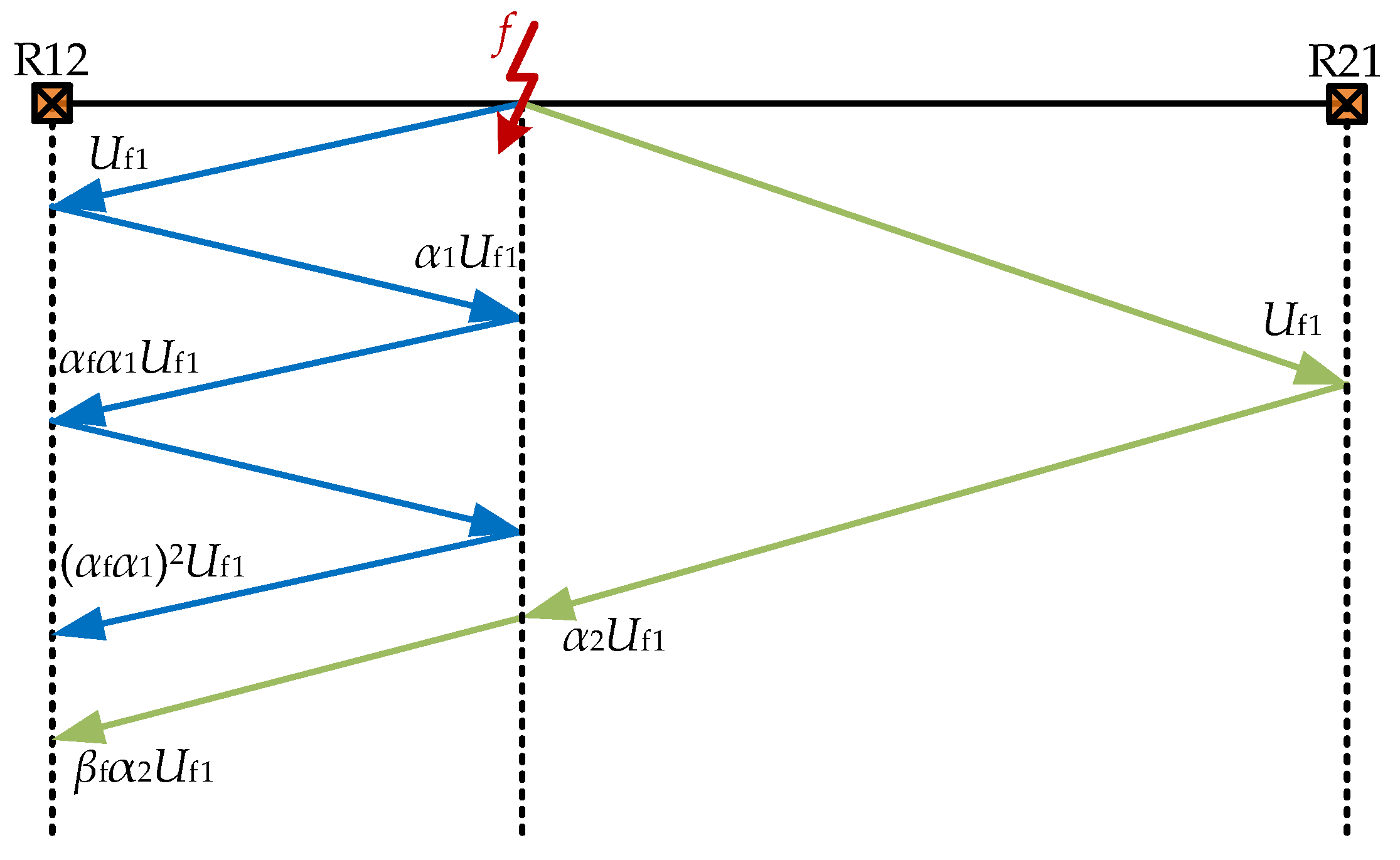
When a fault occurs at the near or far end of a DC line, the electrical distance between the fault point and the line boundary (e.g., current-limiting reactors and converter stations) is extremely short. According to the TW propagation equation, when transient fault-generated TWs propagate along the line to nodes where the wave impedance changes abruptly, continuous TW refractions and reflections occur. To clarify this physical process, a schematic diagram illustrating the TW propagation paths in the studied system topology is shown in
Figure 9.
In
Figure 9,
α1 and
α2 represent the reflection coefficients at the line boundaries,
αf represents the reflection coefficient at the fault point, and
β represents the refraction coefficient at the fault point.
These effects obscure the single- and double-exponential characteristics of the reverse TWs of the fault. If data are directly input into the numerical fitting model, a large model mismatch error will occur, and thus the protection algorithm will not be operated correctly. For an external fault at the bus, the initial TW reaches the measurement point in 0.66 ms (200 km/300 km/ms), while the first reflected TW returns after 1.33 ms. Since the data window of the proposed scheme is only 1 ms, the waveform captured under external faults only contains the initial TW and no subsequent refractions or reflections. For internal faults near line terminals, however, reflected TWs arrive within 1 ms, hence the need for adaptive preprocessing [
24].
The adaptive constant-value flattening method dynamically determines the natural attenuation region of the initial TW, and this region is used as a reference to identify whether subsequent waveform distortion is caused by reflection and refraction. Let the intercepted 1 ms discrete reverse TW sequence be
uF(
n),
n ∈ [1,
N], where
N is the total number of sampling points. Since the leading edge of the initial reverse TW is extremely steep, the algorithm first identifies the first amplitude extremum
uext = max{|
uF(
n)|} within a very short window
Tsearch (0.2 ms in this study) after the fault occurs.
Tsearch must be set such that the first true extremum is reached before the search ends, but before any reflected TWs arrive at the measurement point. For the 150 mH, 200 km system studied, 0.2 ms satisfies both constraints under all simulated conditions. Once the extremum is locked within this window, any subsequent abrupt change in waveform triggers the constant-value flattening. Using this extremum as a reference, a dynamic extremum tolerance band is adaptively established to define the typical fluctuation region of the initial TW without reflection interference. The upper
Uup and lower
Udown bounds of the band are defined as follows:
where
κ is the dynamic tolerance coefficient (0.05 in this study), which is used to accommodate waveform broadening under different fault distances, and
ε is a fixed noise margin, which is used to increase robustness against measurement noise.
After the tolerance band is established, the algorithm monitors the amplitude attenuation trajectory of the subsequent waveform in real time. Once the waveform amplitude exceeds the band (i.e., |uF(n)| > Uup or |uF(n)| < Udown), the sampling point is identified as a sudden-change point nm, caused by the refraction and reflection of the TW.
To completely isolate reflection and refraction interference, maintain the continuity of the voltage waveform, and preserve the fixed sampling length
N required in the subsequent fitting algorithm, an adaptive constant-value flattening step is performed. Specifically, the stable instantaneous value
uF(
nm − Δ
n) before the abrupt change is used to forcibly replace all distorted samples in the interval (
nm,
N]. The corrected waveform sequence
umod(
n) is given in Equation (12):
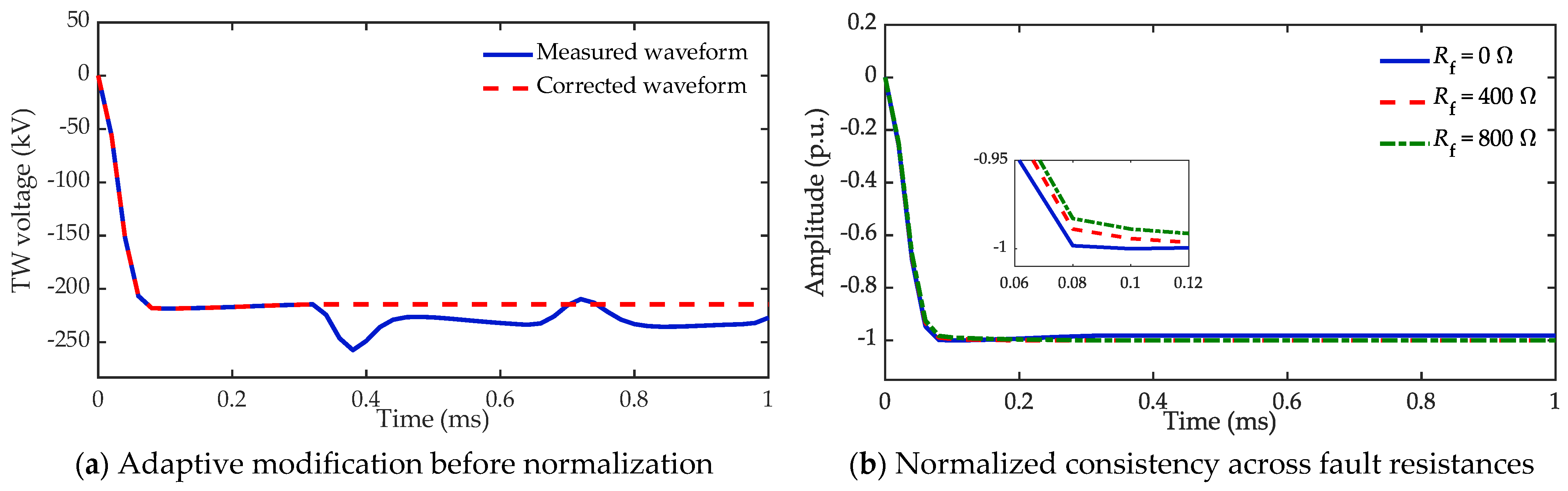
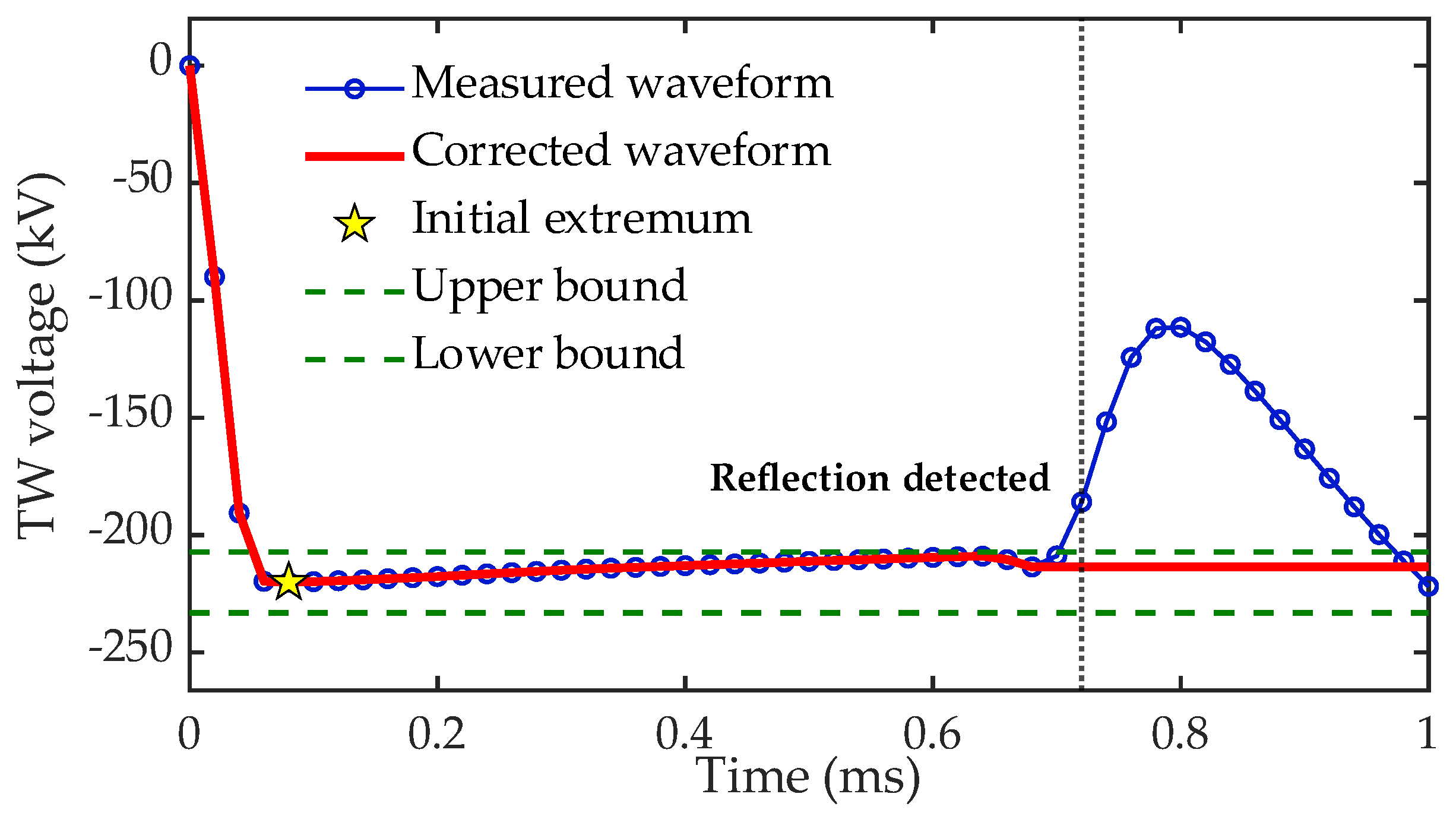
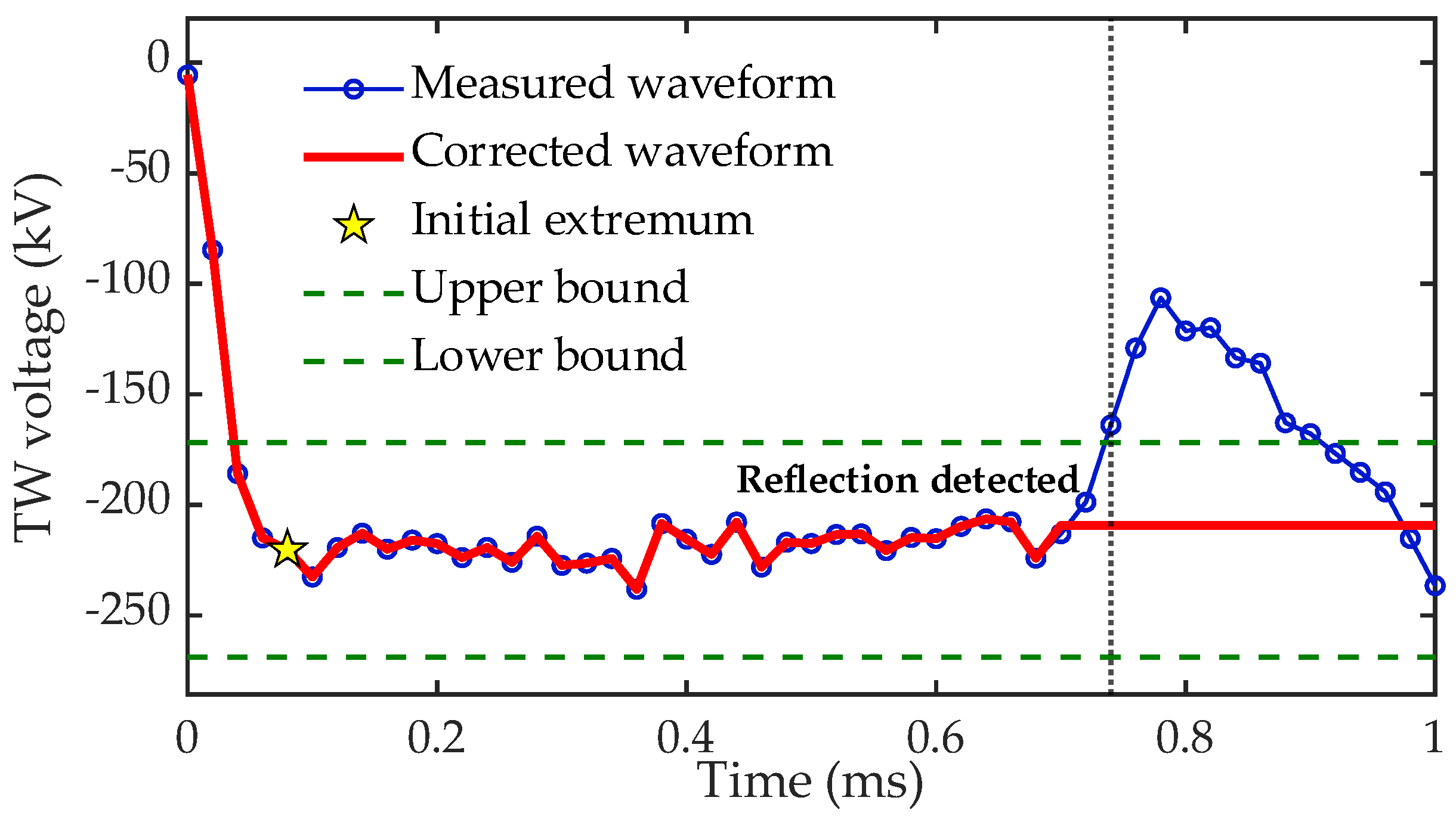
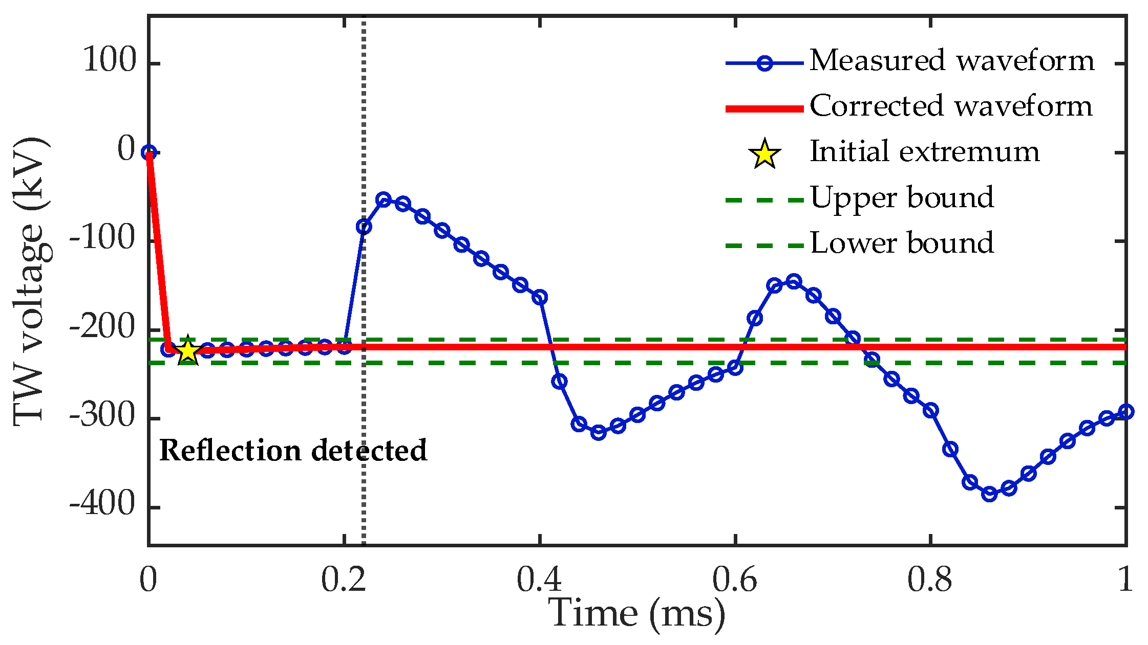
As shown in
Figure 10, this adaptive correction strategy effectively removes interference from waveform reflection and perfectly preserves the exponential attenuation characteristics of the initial TW front.
The tolerance band formed by
κ and
ε also provides inherent noise immunity. As shown in
Figure 11, under 30 dB Gaussian white noise, high-frequency disturbances remain within the tolerance band and do not trigger false flattening, so the normal attenuation of the initial TW is preserved.
For near-end faults, reflected TWs from the remote bus arrive within the data window and distort the waveform. As shown in
Figure 12, when the arriving reflected TW causes the waveform to exceed the tolerance band, the algorithm immediately triggers constant-value flattening, isolating all subsequent reflection interference outside the fitting window while preserving the initial TW’s attenuation trend.
The fault resistance Rf exists only in the multiplicative coefficient term of the waveform expression and mainly affects the amplitude of the TW waveform; it does not alter the time constant (attenuation rate) or the overall trend in the exponential term. To enable the subsequent composite fitting algorithm to compare only the structural characteristics of the waveform, the corrected waveform umod(n) must be normalized.
First, the steady-state mean DC offset
uoffset before the fault transient is calculated and the maximum absolute value of the waveform within the data window is extracted as follows:
Using this value as the reference, the waveform is mapped to the normalized interval of [−1, 0]:
As shown in
Figure 13, after normalization, the differences caused by the amplitude of the fault waveforms under different fault resistances within the same region can be eliminated, thereby increasing the robustness of the subsequent fitting-residual criterion to the fault resistance.
3.2. Definition and Calculation of the Fitting Residuals for Fault Reverse Traveling Waves
To quantitatively extract the differences in the structural characteristics of the waveforms of internal and external fault-generated TWs, fitted waveforms are subtracted from the measured values to obtain the sum of the squared residuals, which reflects the degree of deviation in the physical characteristics of the waveforms.
Let the measured discrete-voltage reverse TW sequence after adaptive flattening and normalization be denoted as
ynorm(
ti), where
i ∈ [1,
n] and
n is the total number of sampling points within the 1 ms data window. If a specific theoretical model
f(
ti,
x) is adopted as the standard waveform, the objective of the nonlinear fitting process is to find an optimal parameter set
x such that the sum of the squared errors (SSE) between the measured waveform and the fitted waveform is minimized. The objective function can be defined as follows:
where
SSE(x) is the calculated sum of the squared residuals;
f(
ti,
x) is the theoretical standard function to be fitted (e.g., a single- or double-exponential function); and
x is the parameter matrix to be determined.
3.3. Principle of the LM Algorithm and Analysis of Its Limitations Under Low-Resistance Conditions
Nonlinear fitting algorithms can adaptively approximate measured waveforms. Let the standard fitting function be
f(
ti,
x). For a fault reverse TW model containing exponential attenuation terms, parameter estimation is essentially a nonlinear least-squares optimization problem. The objective function is defined as minimizing the sum of the squared errors
S(
x):
where
yi is the normalized measured sequence;
f(
ti,
x) is the standard nonlinear fitting function;
x is the parameter vector to be estimated; and
ε(
x) is the residual vector.
The LM algorithm is a nonlinear optimization algorithm that combines global search capability with fast local convergence. During the iterative optimization process, the algorithm performs a first-order Taylor expansion of the nonlinear function at the current parameter
x and introduces a damping factor
μ to control the iteration step size Δ
x. The main parameter update is formulated as shown in Equation (17):
where
J is the Jacobian partial derivative matrix of function
f with respect to parameter
x and
I is the identity matrix.
When the iteration point is far from the optimal solution, the damping factor μ is relatively large and the matrix can be approximated as μI, yielding an updated step size of Δx ≈ −J′ε(x)/μ. In this case, the algorithm functions as a gradient descent method, ensuring that the search proceeds stably along the descending direction while avoiding entrapment in local minima. When the iteration point approaches the optimal solution, μ tends toward 0, yielding an updated step size of Δx = −(JTJ)−1JTε(x). At this stage, the algorithm seamlessly switches to the Gauss-Newton method, and the second-order derivative approximation is used to achieve fast convergence.
This iterative process continues until the predefined convergence criterion is met. For the proposed algorithm, the termination conditions are specified as follows: the iteration stops when the relative change in the objective function tolerance is less than 10−6 or the maximum number of iterations (50) is reached. The output parameter set x at this stage represents the optimal fitting result.
Considering the LM algorithm’s insensitivity to initial values and strong robustness, it is employed as an offline calibration tool. Through nonlinear full-parameter optimization based on the fault data, the inherent attenuation constants λ characterizing different fault types—namely the double-exponential attenuation parameter λdouble for external faults and the typical single-exponential attenuation parameter λsingle for internal faults—can be accurately extracted at different distances.
According to the theoretical foundation presented in
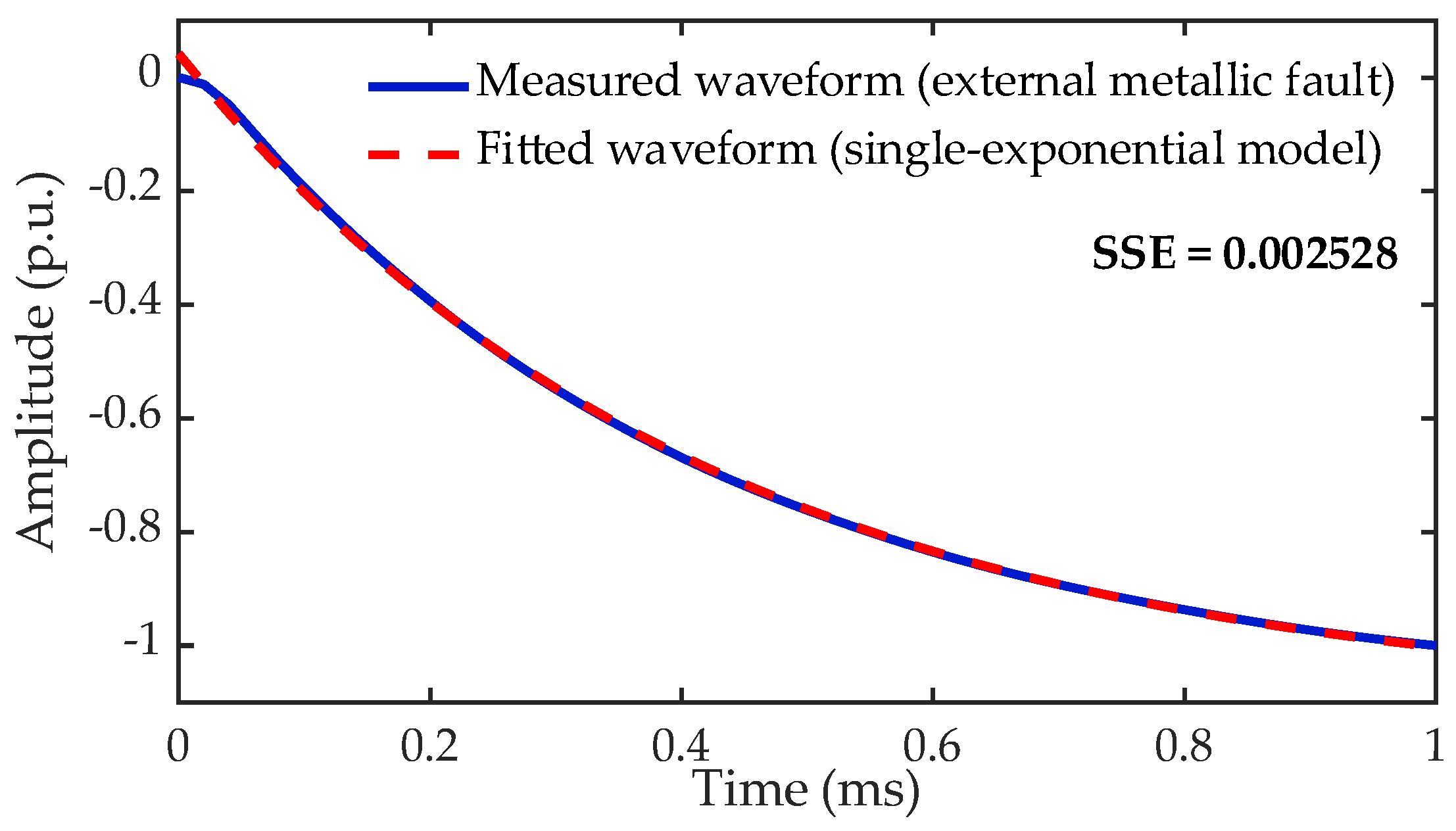
Section 2, external faults inherently exhibit double-exponential attenuation characteristics; thus, fitting them with a single-exponential model should theoretically result in a very large sum of squared residuals. However, extensive electromagnetic transient simulations reveal that when faults with relatively small fault resistance values (such as metallic short circuits and low-resistance grounding faults) occur in the system, the fault reverse TWs attenuate sharply and exhibit extremely smooth waveforms. Under such conditions, the LM algorithm exhibits excellent nonlinear optimization capability. As shown in
Figure 14, when a single-exponential model is used to fit an external metallic fault, the resulting fitting residual SSE is extremely small. This indicates that under low-resistance faults, if a single-exponential model is used to fit the double-exponential waveform of an external fault, the sharply attenuating and monotonically decreasing characteristics of the fault reverse TW result in a relatively good fit for the single-exponential model, yielding an extremely small SSE. Consequently, the sums of the squared fitting residuals for internal and external faults are extremely similar under low-resistance conditions, severely threatening the reliability of the single-ended protection criterion.
3.4. Composite Fitting Strategy Based on the LM and PINV Algorithms
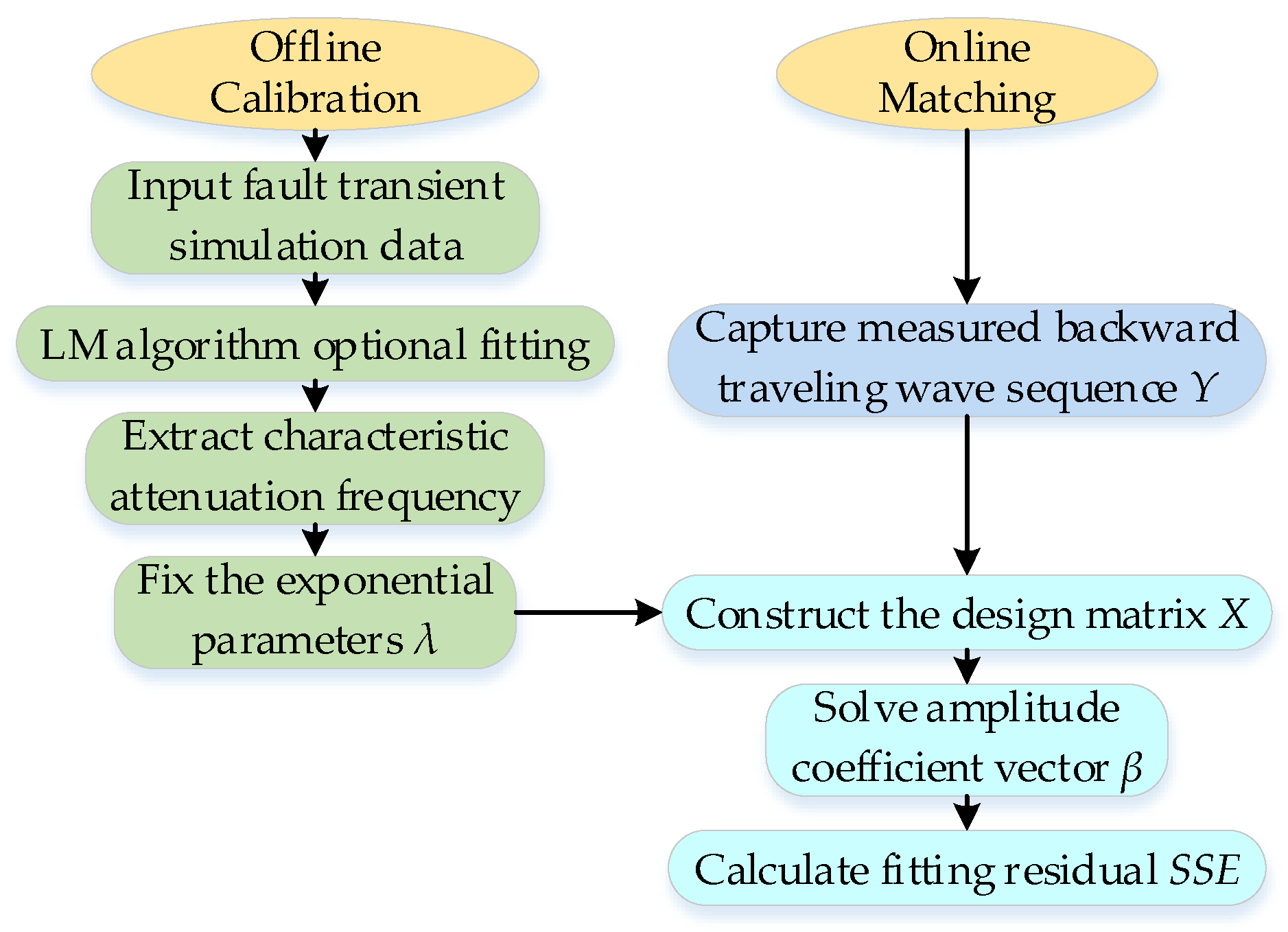
To overcome the problem of the inability to distinguish internal and external faults under low-resistance faults and accurately amplify the differences in the waveform characteristics of internal and external faults, a composite fitting strategy that combines the LM and PINV algorithms is proposed, as shown in
Figure 15. In this strategy, the LM algorithm is used to extract the fixed characteristic exponential parameters, and the PINV algorithm is subsequently employed for online matching. The LM algorithm is a nonlinear dynamic iterative optimization method, and its variables include the exponential parameter (attenuation frequency
λ), which determines the waveform structure. Meanwhile, the PINV algorithm is a direct linear algebraic solution method. In the exponential fitting model, if the nonlinear attenuation frequency parameter
λ is known and fixed, the original model can be reduced to a purely linear combination model with respect to the amplitude coefficients. In this case, the PINV algorithm can be directly applied to obtain a solution, thereby avoiding the divergence and overfitting problems that may arise from nonlinear iterative optimization.
Fault reverse TW simulation data under different fault locations and fault resistances were extracted and the LM algorithm was used to perform unconstrained fitting of the internal and external fault waveforms using the single- and double-exponential models, respectively. The statistical results show that despite the varying operating conditions, the attenuation frequency λ is consistently within a specific numerical range. On the basis of this statistical regularity, representative fixed characteristic exponential parameters (namely, the single- and double- exponential fixed parameters for internal and external faults (λsingle and λdouble1 and λdouble2), respectively) are determined within the corresponding numerical range by considering both the concentrated parameter distribution and the coverage of the fault-distance boundaries. Specifically, for internal faults, a finite set of single-exponential fixed parameters capable of being adapted to the far- and near-end boundaries are selected; for external faults, a combination of double-exponential fixed parameters located at the center of the stable concentrated distribution are selected and fixed in the single- and double-exponential models.
At this stage, the fitting function can be uniformly expressed as an overdetermined system of linear equations:
where
Y is the measured normalized waveform column vector containing
N sampling points,
X is the design matrix composed of the time series
t and the fixed attenuation parameter
λ, and
β is the linear amplitude coefficient vector to be solved.
Using the double-exponential model as an example, the fixed attenuation parameters
λdouble1 and
λdouble2 are used to construct the known design matrix
Xdouble:
Let the normalized column vector of the online measured waveform be
Y. The pseudoinverse matrix
X+ is used to directly and uniquely solve for the linear amplitude coefficient vector
β:
Then, the fitted waveform
Ydouble can be generated as follows:
Subsequently, the SSE under the constraint of the fixed-parameter combination of the double-exponential model is calculated as follows:
The
SSEsingle value for the single-exponential model can be calculated similarly. As shown in
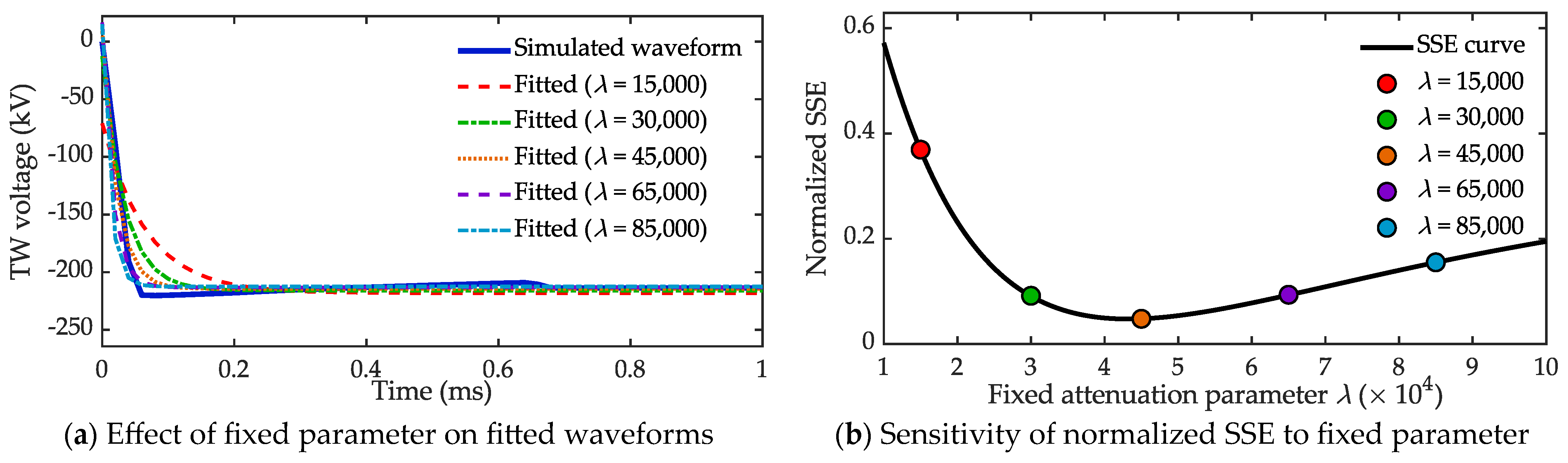
Figure 16, the selected attenuation frequency
λ has a certain influence on the final fitting residual SSE. The results of extensive simulations demonstrate that even under extreme conditions with low fault resistance, this mechanism can still reliably discriminate between the SSEs of the two exponential models.
The proposed scheme comprises offline and online stages. In the offline stage, λsingle and λdouble are determined via LM fitting and loaded into the relay before operation, consuming no online time. In the online stage, the PINV algorithm is applied. At 50 kHz, the 1 ms window contains 50 points (N = 50). Since λ and t are fixed offline, the pseudoinverse matrices are precomputed as constants. Only three matrix–vector multiplications are needed online, requiring less than 100 μs. As a single-ended method with no inter-station communication, the total operating time is approximately 1.1 ms.
4. Principle of Single-Ended Protection Schemes Based on the Composite Fitting Residuals of the Fault Reverse Traveling Wave
4.1. Start-Up Criteria
During normal operation, the pole voltage may exhibit small fluctuations due to load changes or system regulation. To avoid frequent false triggering under steady-state disturbances while maintaining sufficient sensitivity for high-resistance grounding faults, the instantaneous variation in the pole voltage is used to create the start-up criterion as follows:
where
Uref is the rated DC voltage of the flexible DC system and
dU(
i) is the instantaneous variation in the pole voltage detected at the protection installation location. When the variation in the voltage drop exceeds the preset threshold, the protection program is triggered.
4.2. Criterion for Internal and External Fault Identification
After data preprocessing is completed, the main aim of the protection scheme is to accurately distinguish whether the fault on the DC line is internal or external. As described in
Section 3, the composite LM–PINV fitting algorithm is used to amplify the residual differences between internal and external faults. Its main logic consists of two steps: offline extraction of fixed characteristic exponential parameters and online matching.
In the offline parameter extraction stage, the LM algorithm is used to perform unconstrained fitting on the fault reverse TWs simulated under different fault resistances (0–800 Ω) and fault distances (0–200 km). The statistical results show that for internal faults, owing to the influence of the fault distance, the attenuation parameter of the single-exponential model exhibits a wide distribution range. Specifically, the larger the fault distance, the more severe the attenuation and the smaller the optimal parameter, with this value approaching 30,000. In contrast, the smaller the fault distance, the steeper the waveform and the larger the optimal parameter, with this value approaching 100,000. For external faults, owing to the smoothing effect of the current-limiting reactor at the line boundary, the parameters of the double-exponential attenuation model are highly concentrated within specific ranges, and the optimal double-exponential attenuation parameters λdouble1 and λdouble2 remain stable around 900 and 2000, respectively.
In the online matching stage, if only a single fixed attenuation parameter is used to constrain the fitting, deviations in the actual faults increase the fitting residuals of the internal faults, thereby reducing the distinguishability between internal and external faults. To ensure the sensitivity of the identification results across the entire line and the full range of fault resistances, the following parameter combinations are selected based on the parameter ranges obtained from the offline step to construct a parameter combination design matrix.
For the double-exponential model, the parameters λdouble1 = 5000 and λdouble2 = 2500 are fixed to construct the double-exponential design matrix Xdouble, and SSEdouble is calculated. When the convergence tolerance is strictly set to 10−6, the optimal parameters concentrate around λdouble1 = 900 and λdouble2 = 2000; however, this combination poses a risk of overfitting. To improve robustness, the tolerance was relaxed to 10−4, under which the algorithm converges to λdouble1 = 5000 and λdouble2 = 2500. This combination still leads to the accurate characterization of external fault waveforms while reducing overfitting risk.
For the single-exponential model, to cover faults at different distances, two sets of independent parameters, λsingle1 = 30,000 (for long-distance far-end faults) and λsingle2 = 60,000 (for short-distance near-end faults, extended to 65,000 under high-resistance conditions), are selected. Accordingly, two single-exponential design matrices, Xsingle1 and Xsingle2, are constructed, and their respective residuals SSEsingle1 and SSEsingle2 are calculated using the PINV algorithm.
For any internal fault, its waveform is expected to closely match at least one of the two single-exponential parameter settings (
SSEsingle1 and
SSEsingle2). Therefore, the smaller of the two is taken as the final representative value of the single-exponential fitting residual:
The residual ratio discrimination coefficient
Kdist is constructed as follows based on the strong matching mechanism of the composite fitting algorithm:
Finally, a discrimination threshold is defined on the basis of the above findings. When the criterion in Equation (28) is satisfied, the fault is identified as an internal fault of the DC line:
where
εset is the reliable operating threshold used in this study.
4.3. Fault Pole Selection Criterion
After identifying an internal fault, the fault pole must be determined to enable single-pole tripping or bipolar blocking. According to phase-mode transformation, the zero-mode voltage u0 equals the sum of the positive- and negative-pole voltages. Under a positive PGF, the positive-pole voltage drops while the negative-pole remains stable, causing the zero-mode voltage to exhibit negative polarity. Under a negative PGF, the opposite occurs, producing positive polarity. Under a pole-to-pole fault (PPF) or simultaneous bipolar grounding fault, both pole voltages decrease symmetrically, and the zero-mode voltage ideally cancels out to nearly zero.
Therefore, the algebraic sum of the discrete zero-mode voltage samples within the data window is extracted to construct the fault pole-selection criterion:
where
N is the number of sampling points in the data window and
Pset is the reliability threshold. To avoid erroneous pole selection due to unbalanced zero-mode voltage under external disturbances or PPFs,
Pset is determined based on the maximum possible unbalanced zero-mode voltage in the system.
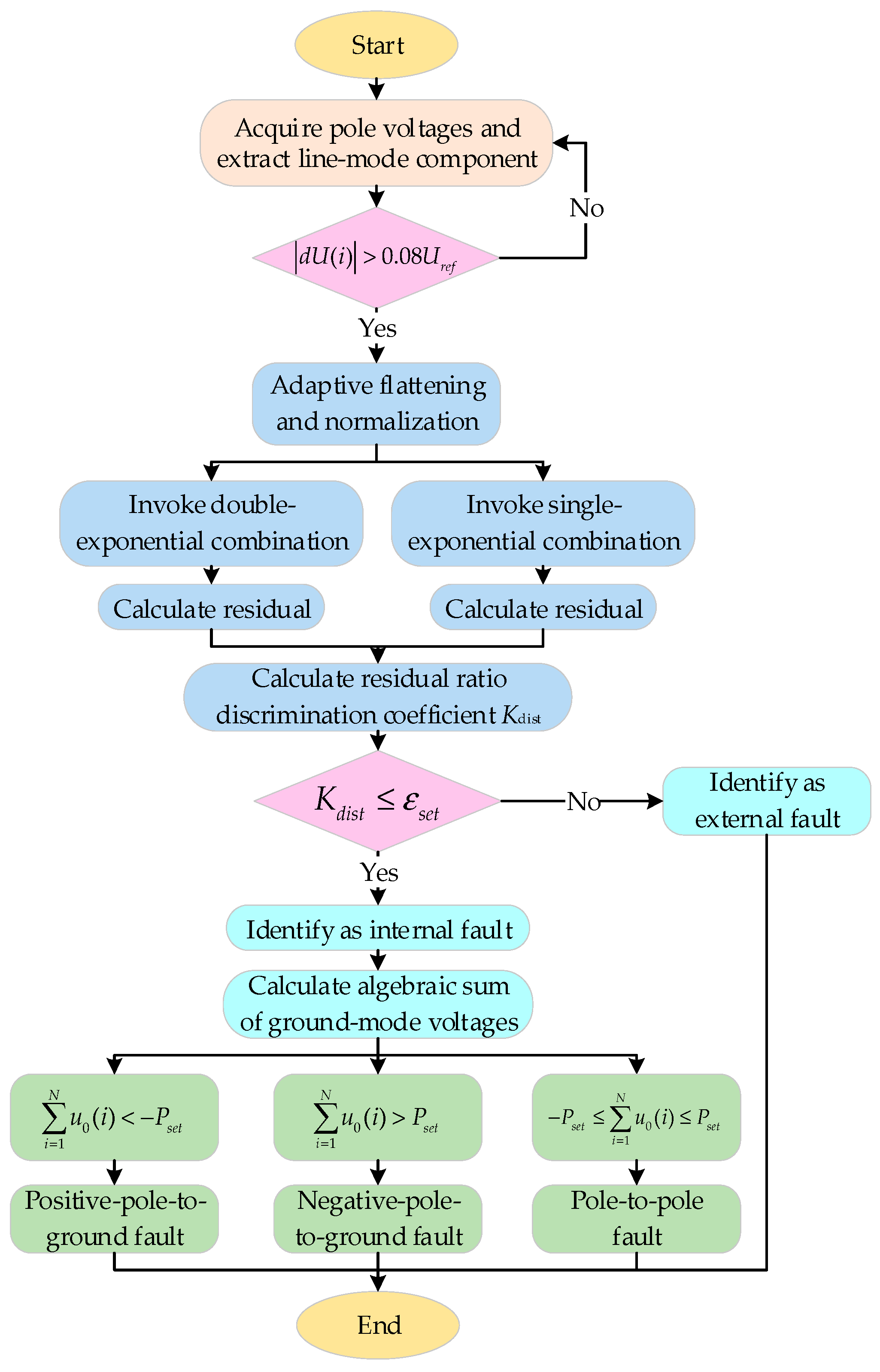
The overall protection procedure is shown in
Figure 17.
5. Simulation Verification
PSCAD/EMTDC is widely recognized as the mainstream electromagnetic transient simulation tool in both industry and academia, and can accurately reproduce the electromagnetic transient evolution process of flexible DC transmission systems under various operating conditions. Regarding the flexible DC line fault protection method investigated in this study, this software fully accounts for the frequency-dependent parameters of transmission lines, precisely characterizing the attenuation, refraction, and reflection behavior during TW propagation. Furthermore, it supports detailed modeling of MMC stations and their associated control loops, accurately reflecting the dynamic response of various system electrical parameters throughout the fault transient process.
To verify the adaptability of the proposed protection scheme, a ±400 kV symmetrical four-terminal flexible DC grid was built in PSCAD/EMTDC, and its topology is shown in
Figure 1. The system parameters of the simulation model are listed in
Table 1. The J. Marti frequency-dependent parameter model was adopted for the DC transmission lines, the sampling frequency was set to 50 kHz, and the data window length was 1 ms.
5.1. Setting Principles for Protection Thresholds
5.1.1. Setting Principle for the Discrimination Threshold εSet
Kdist is defined as the ratio of the single-exponential fitting residual to the double-exponential fitting residual. For an internal fault, the voltage reverse TW follows a single-exponential decay, and the single-exponential model fits this well, yielding a small SSEsingle and a large SSEdouble. Thus, Kdist approaches 0. For an external fault, the voltage reverse TW follows a double-exponential decay, and the single-exponential model fits this poorly, yielding a large SSEsingle and a small SSEdouble. Thus, Kdist is substantially greater than 1. This difference in fitting capability between the two models is therefore exploited in the criterion to discriminate fault types.
The threshold must account for both extreme scenarios. To ensure reliable identification of external faults,
εset must be smaller than the minimum
Kdist of external faults under the most adverse conditions:
where
min(
Kdist_external) denotes the lowest
Kdist of external faults under all adverse conditions and
Krel is the reliability coefficient. External-fault simulation cases spanned fault resistances of 0–100 Ω and fault locations of 0–200 km, and extensive simulations yielded
min(
Kdist_external) = 3.157. A reliability coefficient of
Krel = 6 is adopted, and after rounding,
εset ≈ 0.5.
To prevent maloperation under internal faults, εset must also be verified against the most adverse internal faults. Internal-fault simulation cases spanned 0–800 Ω and 0–200 km, yielding max(Kdist_internal) = 0.173. The sensitivity margin is Ksen = εset/max(Kdist_internal) >> 2, far exceeding the required protection sensitivity. The maximum discriminant value under internal faults thus remains substantially smaller than εset. The selected threshold ensures a sufficient discrimination margin between the most severe internal and external faults.
5.1.2. Setting Principle for the Pole-Selection Threshold Pset
The pole selection criterion is based on the polarity characteristics of the zero-mode voltage. For a positive PGF, the positive pole voltage drops rapidly and the zero-mode voltage exhibits a pronounced negative mutation, while for a negative PGF, the negative pole drops and the zero-mode voltage exhibits a pronounced positive mutation. For a PPF, both poles drop nearly symmetrically, and the zero-mode voltage should theoretically be zero.
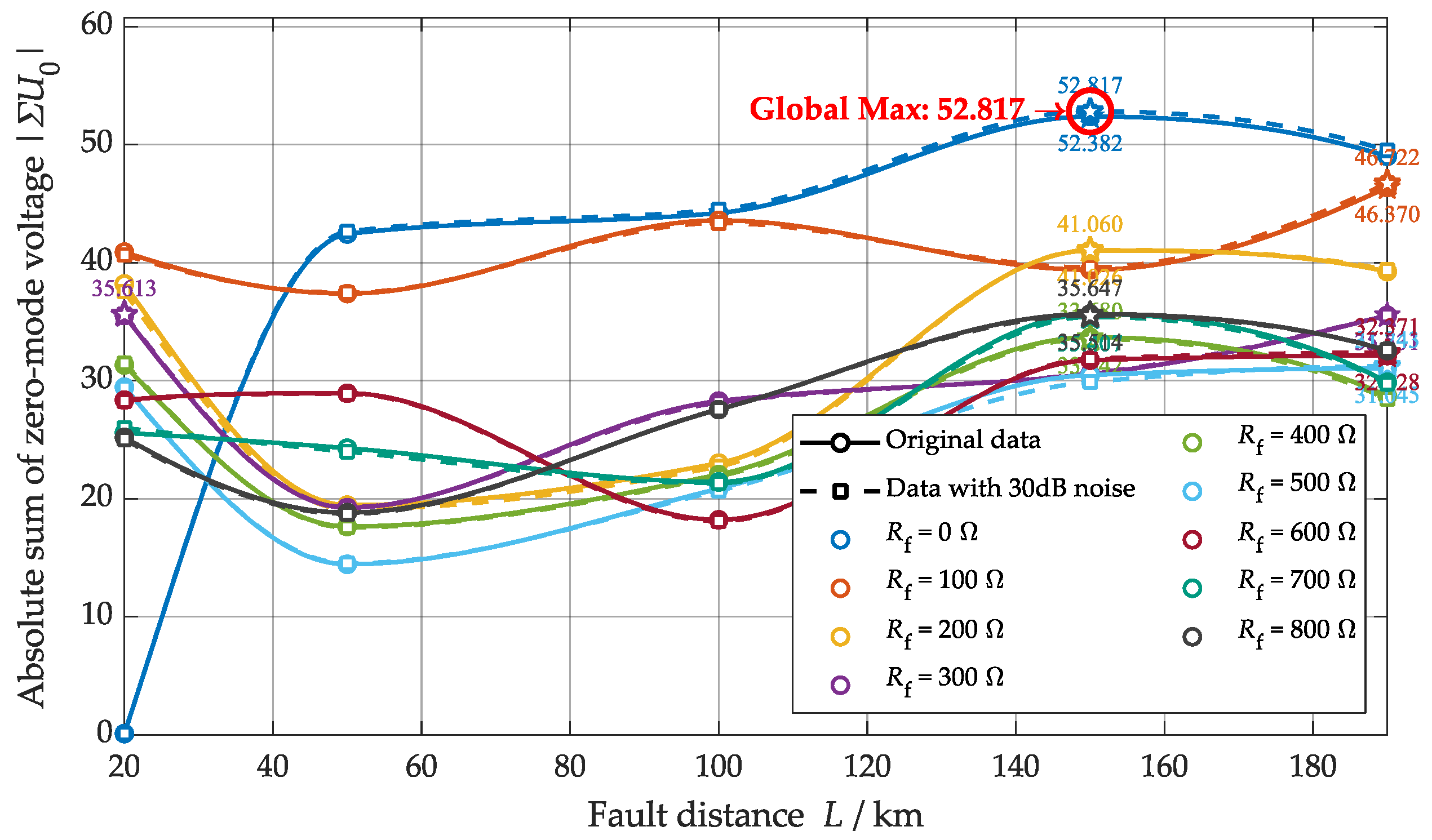
In practice, however, due to line parameter asymmetry, measurement errors, and noise, the integrated zero-mode voltage exhibits residual fluctuations rather than being strictly zero within 1 ms after a PPF. Therefore,
Pset must be set to reliably endure the maximum zero-mode voltage integral that may appear under internal PPF conditions. PPFs were simulated across fault locations of 0–200 km and fault resistances of 0–800 Ω, with 30 dB Gaussian white noise. The maximum absolute integral within the 1 ms window is statistically evaluated, as shown in
Figure 18.
Introducing a reliability coefficient
Krel = 1.5, the threshold is set to
Pset = 78.6:
Using this value, Pset effectively covers the range of the zero-mode voltage fluctuations under PPF conditions, ensuring reliable pole selection and avoiding misjudgment between single-pole grounding faults and bipolar short-circuit faults.
5.2. Analysis of the Effectiveness of the Proposed Protection Scheme
The test results show that the proposed protection scheme operates normally under an 800 Ω internal fault and a 100 Ω external fault. The results of testing the proposed protection scheme under various faults are presented in
Table 2. Fault locations include the near end of the line (20 km, 50 km, 100 km, and 150 km), the far end of the line (190 km), and the outlet of the remote converter station and the internal fault resistances are set to 0 Ω, 400 Ω, and 800 Ω, while the external fault resistances are set to 0 Ω, 10 Ω, and 100 Ω. Two fault types, PGF and PPF, are considered.
As shown in
Table 2, the protection measurement point M operates correctly under different fault locations, types, and resistances.
Figure 19 shows the correlations between the residual ratio discriminant coefficient
Kdist and the fault location and fault resistance under different faults. As shown in
Figure 19a,b, for internal faults at different locations and with various resistances, the
Kdist curves remain relatively stable and exhibit consistently low values, which are far below the operating threshold, thereby preserving the large sensitivity margin. Furthermore, as shown in
Figure 19c, for external faults with different resistances, the
Kdist values are significantly higher than the operating threshold under low-resistance faults, thereby increasing the operating margin and robustness of the protection scheme.
5.3. Analysis of the Performance of the Proposed Protection Scheme
5.3.1. Noise Interference
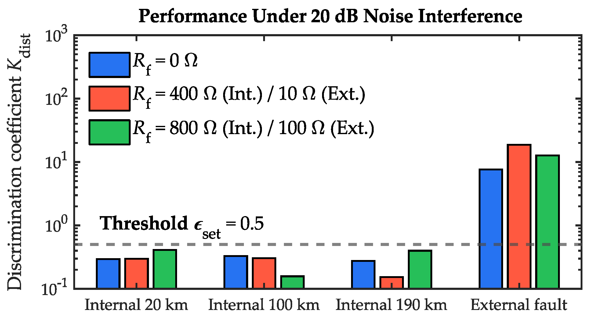
Noise is present in actual signals and may affect the fault identification results by altering the overall waveform characteristics. However, the adaptive flattening method adopted in this study can effectively suppress noise interference, thereby increasing the robustness of the proposed protection scheme to noise. Gaussian white noise with a signal-to-noise ratio (SNR) of 20 dB was added to the measured signals to evaluate the performance of the proposed protection scheme under noisy conditions. The test results show that the proposed method can still accurately identify faults under these noise conditions (
Figure 20), indicating that it possesses strong anti-noise interference capability.
5.3.2. Current-Limiting Reactor
The main difference between internal and external faults lies in the effect of the current-limiting reactor on fault-generated TWs. To verify the adaptability of the proposed method under different reactor values, tests were conducted with a reactance of 50 mH. The results in
Table 3 show that the reactor only has a slight influence on internal fault identification, whereas for external faults, the protection performance improves with increasing reactance. Overall, the proposed method still performs well for DC systems with weak boundary characteristics, such as a 50 mH current-limiting reactor.
5.3.3. Transmission Line Length
The transmission line length affects the attenuation and waveform characteristics of transient TWs. As the line length increases, dispersion and dielectric loss become more significant, resulting in a slower leading edge and a reduced initial TW amplitude. To verify the adaptability of the proposed scheme to long-distance lines, simulations were conducted after increasing the line length from 200 km to 400 km; other parameters were unchanged.
Table 4 presents the calculated
Kdist values for a 400 km line. These results show that the difference in fitting residuals between internal and external faults remains highly significant, and the proposed protection scheme reliably identifies various faults with sufficient operating margins.
5.3.4. Two-Terminal Symmetrical Bipolar MMC-HVDC Transmission System
To verify the adaptability and robustness of the proposed single-ended protection scheme across different HVDC system topologies, extensive additional simulation tests were performed for a two-terminal symmetrical bipolar MMC-HVDC transmission system. The corresponding test results are shown in
Table 5 and demonstrate that the proposed single-ended protection scheme maintains high reliability in the two-terminal system across various fault resistances and distances. The discriminant coefficient
Kdist exhibits a clear distinction between internal and external faults, demonstrating that the proposed scheme is adaptable to different HVDC system topologies.
5.4. Comparison with Existing Protection Schemes
To demonstrate the superiority of the proposed scheme, it was compared with existing protection schemes.
5.4.1. Comparison with a Voltage Derivative-Based Protection Scheme
In reference [
25], voltage derivative-based protection was utilized as the primary protection scheme for HVDC transmission lines. Through this scheme, the voltage derivative is extracted by calculating the derivative of the measured voltage at the relay location, and the protection threshold is determined based on the characteristic quantity extracted under the most severe external fault conditions. Its operating criterion is defined as follows:
where
εth represents the setting threshold of the voltage derivative;
duex/
dt is the maximum absolute voltage derivative under external faults; and
Krel denotes the reliability coefficient, which is set to 1.4.
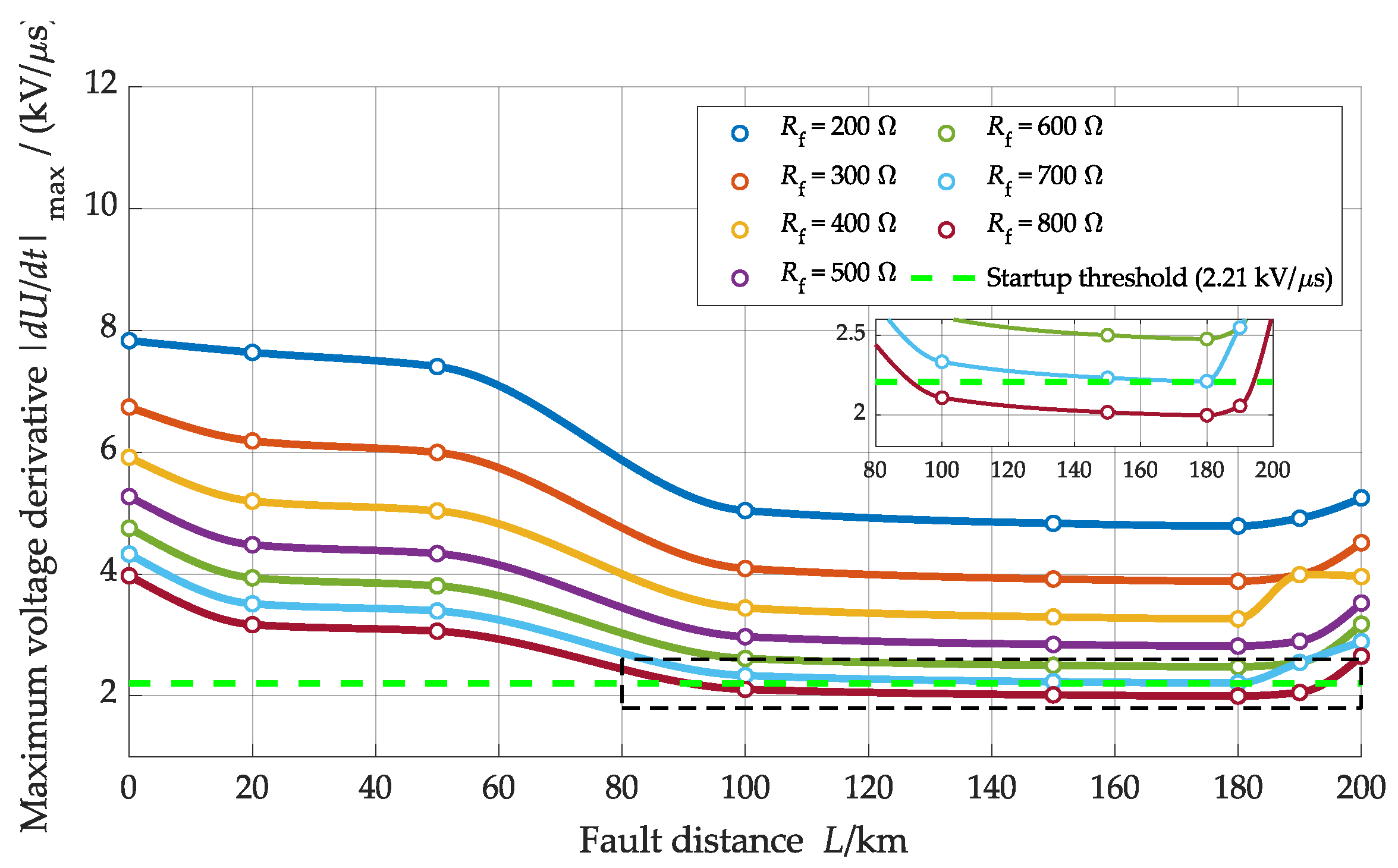
Figure 21 illustrates the maximum voltage derivative across different fault resistances and fault distances.
As shown in
Figure 21, the voltage derivative protection method only reliably identifies internal faults when the fault resistance is between 0 and 600 Ω. When a fault exceeding 600 Ω occurs at the far end, this method fails. The main reason is that the high-frequency components of the initial voltage TW attenuate due to the combined effects of line distributed capacitance and fault resistance during propagation, significantly smoothing the TW front and reducing the voltage derivative amplitude.
In contrast, our proposed scheme effectively reduces the impact of fault resistance on the characteristic quantity amplitude through the first step of normalization. Moreover, rather than relying on a single numerical threshold at a specific instant, our method uses the evolutionary pattern of the fault waveform across the entire time window for fault discrimination. Therefore, it reliably distinguishes internal and external faults even under a fault resistance of 800 Ω.
5.4.2. Comparison with an Exponential Coefficient-Based Single-Ended Protection Scheme
The scheme in reference [
20] uses a standard fitting function as the reference and applies the LM algorithm to perform exponential fitting on the fault voltage waveform, thereby extracting the propagation exponential coefficient of the line-mode fault voltage TW. The protection threshold is set based on the maximum exponential coefficient extracted under external faults:
where
Idex_external is the maximum absolute exponential coefficient under external faults and
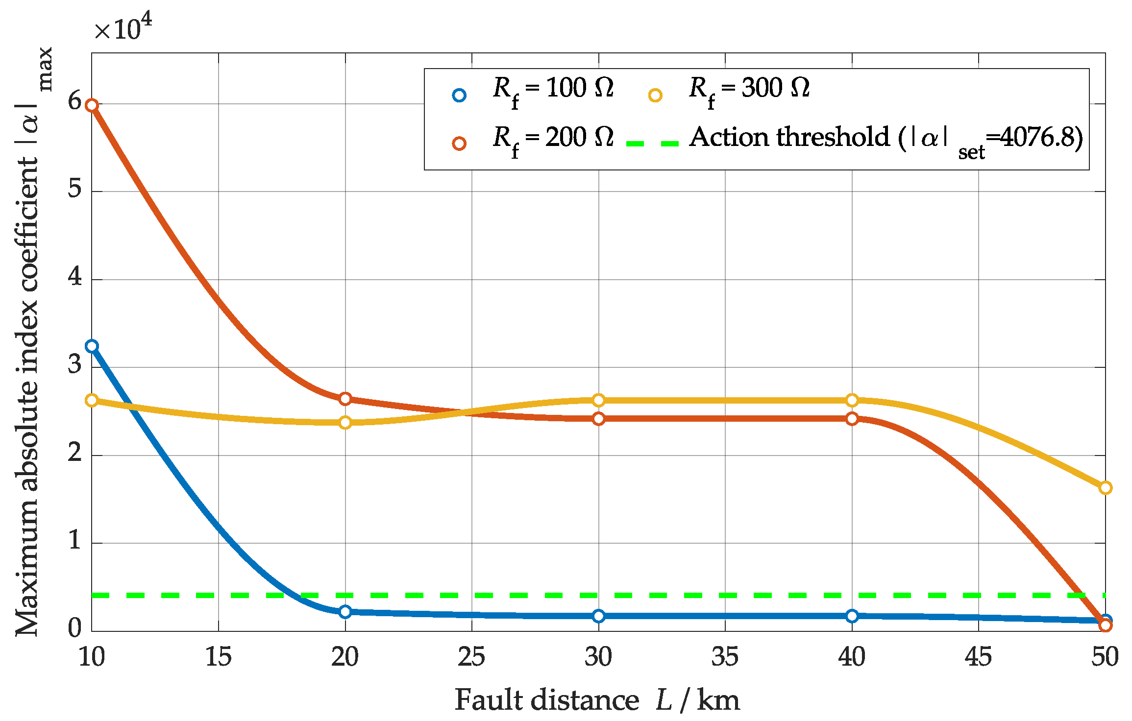
Krel is the reliability coefficient, set to 1.2. The scheme was tested across different fault resistances and fault distances under the same sampling frequency and system conditions, as shown in
Figure 22.
As shown in
Figure 22, this method extracts large exponential coefficients and operates reliably under near-end and metallic faults. However, as the fault distance increases and fault resistance is introduced, its performance degrades, failing for 100 Ω and 200 Ω faults at 10 km and 50 km. The primary cause of this is that for near-end faults, refracted and reflected TWs enter the sampling window alongside the initial TW. When the LM algorithm is applied for exponential fitting, these TWs disrupt the exponential decay pattern, leading to a degraded fitting accuracy or even fitting failure.
In contrast, the proposed scheme introduces an adaptive correction mechanism that promptly identifies and suppresses the effects of subsequent TW refractions and reflections. This mechanism restores its intrinsic decay characteristics while preserving the features of the initial reverse fault TW, thereby avoiding interference from TW refractions and reflections and ensuring accurate fault feature extraction.
5.4.3. Comparison with an Exponential Fitting Residual-Based Protection Scheme
The scheme in reference [
21] uses the fitting residuals obtained from the analytical time-domain expression of the external fault reverse voltage TW as the fault characteristic quantity, and a protection criterion is proposed to discriminate internal and external faults.
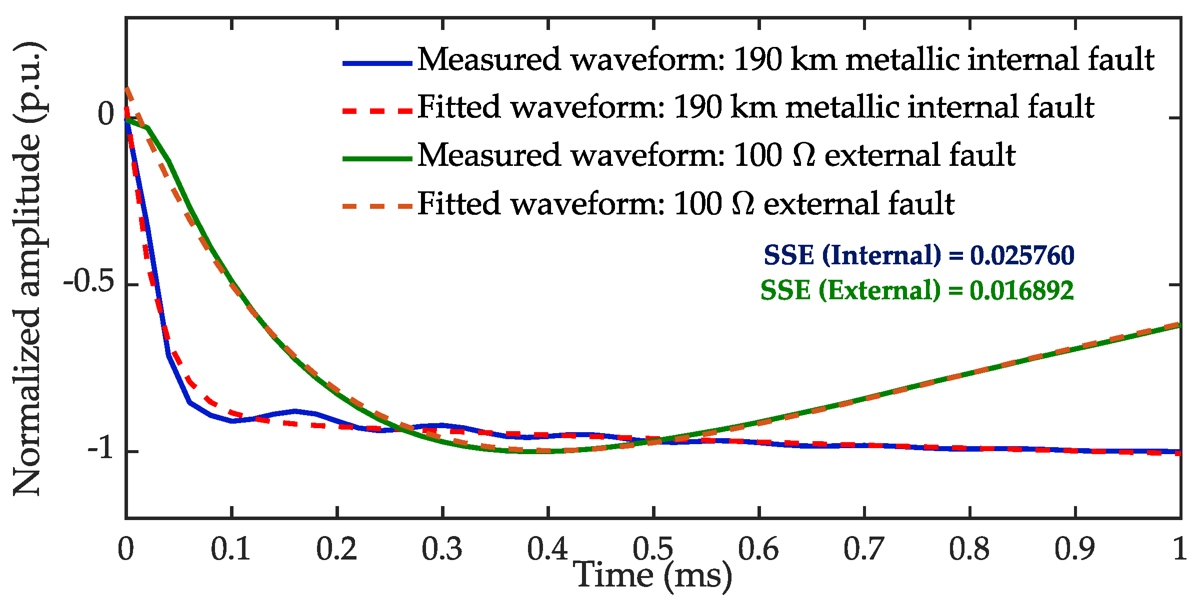
Figure 23 shows the 1 ms measured waveforms under two typical conditions alongside their corresponding double-exponential model fitting curves.
As shown in
Figure 23, the double-exponential model achieves a high fitting accuracy for both fault types, with the fitted curves closely matching the original waveforms. Notably, the fitting residuals for a 190 km internal far-end fault and a 100 Ω external fault are very similar, indicating insufficient discrimination.
When this scheme uses the LM algorithm to optimize parameters for external fault waveforms, the sole objective is to minimize the fitting residual. When the convergence tolerance is set too strict, the LM algorithm tends to overfit the measured waveform, yielding a parameter set with an extremely high fitting accuracy for external faults. Although this parameter set effectively reduces the fitting error for external faults, it inherently weakens the model’s capacity to characterize the features distinguishing different fault types. Consequently, when an internal far-end fault waveform resembles an external fault waveform due to long-distance propagation, the double-exponential model likewise yields a small fitting residual, causing the residual values of internal and external faults to approach each other.
In contrast, in the LM-PINV composite fitting strategy proposed in this paper, the characteristic exponential parameters are extracted and fixed offline, while the PINV algorithm is used for online matching calculation. This effectively overcomes the nonlinear overfitting problem under low-resistance faults and significantly improves the reliability of discriminating between internal and external faults.
6. Conclusions
In this study, fault reverse TWs are analyzed to address the problems of fitting algorithms in single-ended protection schemes for flexible DC transmission lines, namely that they are prone to overfitting under low-fault-resistance conditions and suffer from reduced reliability owing to the interference of refracted and reflected TWs. Accordingly, a single-ended protection scheme based on composite fitting residuals is proposed and validated.
(1) Analytical expressions for the reverse TWs of line-mode voltages under internal and external faults are derived, revealing essential differences in their waveform structural characteristics: internal faults exhibit single-exponential attenuation characteristics, whereas forward external faults exhibit double-exponential attenuation characteristics.
(2) An adaptive traveling wave flattening and normalization preprocessing method is proposed to eliminate the effects of TW refraction and reflection and fault resistance. On this basis, a composite LM–PINV fitting strategy is utilized to calculate fitting residuals through online matching with offline-extracted characteristic parameters to establish protection criteria.
(3) Extensive simulation tests demonstrate that the proposed method effectively identifies various internal and external faults at a sampling frequency of 50 kHz. It successfully eliminates protection dead zones at the near and far ends of the line, reliably protecting the entire transmission line with high sensitivity even under a fault resistance of 800 Ω. Moreover, the protection operates correctly under 30 dB Gaussian white noise interference conditions, demonstrating strong robustness and excellent protection performance.