Multi-Focus Image Fusion Using Soft Decision Maps and Dual Fusion Rules

Abstract

Multi-Focus Image Fusion is a technique that combines the in-focus regions from multiple images of the same scene, captured at different focal planes, to generate a single image with an extended Depth of Field compared to the source images. Despite improved fusion quality, recent approaches are constrained by high computational cost and the need for large training datasets, reducing their feasibility in resource-limited scenarios. In this work, a multi-focus fusion method based on a soft decision map is proposed, where the map is generated from local focus measurements in each scene. Subsequently, two Fusion Rules are employed: the Additive Fusion Rule, commonly used in the state of the art, and the Multiplicative Fusion Rule, which, to the best of our knowledge, has not been previously reported in the MFIF context. The method is evaluated using the public MFI-WHU and Lytro datasets through both reference-based and non-reference metrics. The results demonstrate that the proposed method produces visually coherent fused images and achieves competitive performance in terms of structural similarity, edge preservation, and information content, while maintaining low computational complexity.

1. Introduction

In recent years, conventional optical systems used to capture images of a scene for subsequent analysis have improved significantly. However, one of their main limitations remains the difficulty of achieving an extended Depth of Field without compromising resolution [1]. Techniques involving the acquisition of multiple images at different focus levels using a varifocal lens, combined through weighted superposition, have demonstrated the ability to reduce defocus sensitivity and improve image clarity [2]. Methods based on the use of hyperbolic phase masks in optical systems operating at full pupil apertures have been proposed to control depth of field. These approaches reduce the impact of focus errors while increasing the Modulation Transfer Function, improving image quality [3]. Among the most widely used techniques to avoid the use of special lenses and phase filters is Multi-Focus Image Fusion (MFIF), which aims to integrate multiple images of the same scene captured at different focal planes and subsequently fuse the information using different image-processing and artificial-intelligence techniques [4]. The ability to combine high-resolution information from different regions is essential, as it helps mitigate the loss of relevant information in subsequent analysis or recognition tasks; This capability is particularly important in areas such as microscopy, where structures located at different focal depths must be visualized simultaneously [5]. Similarly, recent MFIF techniques have been applied in systems aimed at preserving discriminative features for computer-vision tasks [6], in methodologies focused on estimating depth information from image sequences or stacks acquired at different focal planes [7], and in real-world scenarios involving complex acquisition conditions, illumination variations, and dynamic scenes that require robust fusion strategies [8].

Traditionally, low-computational-cost and easy-to-implement MFIF methods have relied on the use of Focus Measure Operators (FMO) to estimate the Local Focus Measurement (LFM) in the input images [4]. This principle remains relevant in recent MFIF methods, where focus-aware representations are employed to guide the integration of complementary visual information [9]. Among the most widely used focus-estimation approaches are spatial-domain operators based on local gradients, energy measures, and second-order derivatives. These methods have been extensively employed in MFIF due to their simplicity and effectiveness in detecting focused regions [10]. Statistical focus measures, including variance-based operators, are also widely used to quantify local sharpness and image activity [11]. In addition, frequency-domain and multi-scale approaches have been investigated for focus estimation. Representative examples include methods based on the Fourier transform, discrete cosine transform (DCT), wavelet transform, and other multiresolution decompositions [12]. These methods are well suited for real-time applications due to their efficiency; however, when the Fusion Rule (FR) relies on binary decisions, i.e., selecting the pixel from the source image with the higher focus measure, they may produce abrupt transitions and artifacts in regions where both images exhibit similar levels of sharpness [13]. Subsequently, methods based on multiscale transforms, guided image filtering, cross bilateral filtering, and Gaussian curvature filtering, among others, have been developed to improve spatial consistency and edge preservation. In this context, Ming et al. propose an MFIF method in the Nonsubsampled Contourlet Transform (NSCT) domain [14], where a distance-weighted regional energy measure is used for fusing low-frequency components, whereas a tensor-based structure operator is employed to process high-frequency components, enabling better preservation of details and edges. Additionally, a consistency verification mechanism is incorporated to enhance the robustness of focused region selection. Similarly, Wan et al. develop a multiscale decomposition-based approach that combines energy measures for low-frequency components with a parameter-adaptive pulse-coupled neural network (PA-PCNN) model for high-frequency components [15], effectively reducing artifacts in transition regions. Chen et al. [16], introduce an MFIF algorithm, noteworthy because of its computational efficiency and suitability for real-time processing, based on multiscale feature aggregation, where the input images are first downsampled to estimate local defocus levels using difference-of-Gaussians and Laplacian filters; then, they are upsampled before applying the final decision map. Although these methods represent significant improvements in mitigating abrupt transitions and artifacts in regions with similar sharpness levels, the use of multiscale transforms in most of these approaches considerably increases their computational cost.

Recently, supervised deep-learning approaches have demonstrated the ability to learn focus-related features, improving the preservation of structural details in fused images [17]. In parallel, unsupervised learning methods have emerged as an attractive alternative by eliminating the need for reference-fused images, while achieving competitive fusion performance through task-oriented feature learning and loss functions [18]. In this context, Zhang et al. propose an end-to-end image fusion framework based on a convolutional neural network (IFCNN) [19], in which features extracted from source images are fused using element-wise rules and subsequently reconstructed to generate the final image. This approach eliminates the need for post-processing and enables joint model optimization, while leveraging multi-focus datasets with reference images to improve performance and generalization capability. On the other hand, Xu et al. develop a unified unsupervised image fusion network (U2Fusion) [20], which employs a loss function focused on preserving structural information, thereby removing the need for fully focused reference images during training. Tian et al. [17] propose a two-stage MFIF method that combines a DenseNet-based encoder–decoder network with a polarized self-attention module for image reconstruction, along with a fusion strategy based on edge maps derived from encoded features. These maps enable pixel-level discrimination of focused regions and generate a decision map that guides a weighted fusion process, improving detail preservation and smooth transitions between regions. Liu et al. [18] introduce a multi-focus fusion method based on an encoder–decoder architecture with multiscale residual blocks and hybrid attention, trained in an unsupervised manner. The model incorporates an up-and-down sampling projection (UDP) module to enhance edge information and generates a decision map from feature analysis in the spatial–frequency domain, which guides the final fusion. This approach achieves improved detail preservation and greater robustness in fused image quality. More recently, Xie et al. [21] propose SwinMFF, an end-to-end MFIF framework based on the Swin Transformer architecture. By leveraging self-attention mechanisms to model long-range dependencies across source images, this method improves image fidelity and alleviates boundary artifacts commonly observed in end-to-end fusion approaches. Experimental results demonstrate that SwinMFF achieves competitive performance against a wide range of state-of-the-art methods. Song et al. [22] introduce MLP-MFF, a lightweight end-to-end fusion framework based on pyramidal MLP modules. This approach aims to achieve efficient feature extraction and fusion while reducing computational requirements. Experimental results indicate competitive fusion performance with substantially lower model complexity. However, despite their strong performance, many of these approaches require training processes that involve large volumes of data and substantial computational resources, which may limit their applicability in resource-constrained environments or in scenarios where sufficient data are not available [23].

Considering the previously described scenario, in this work, an MFIF methodology is developed based on a spatial-domain FMO, capable of maintaining low computational cost while achieving competitive performance. To this end, particular attention is given to one of the most critical aspects of the fusion process: the transition from binary decision maps (BDM) to soft decision maps (SDM), which preserve spatial coherence without introducing abrupt transitions or significantly increasing algorithmic complexity. This issue is addressed in this work by formulating a fusion scheme based on an LFM derived from the Tenengrad criterion [11]. Specifically, energy maps are generated for each source image, from which an SDM is constructed to guide the fusion process through a novel FR. This proposed approach effectively reduces the presence of artifacts. Additionally, two FR are analyzed: the widely used linear additive interpolation and the proposed Multiplicative FR. Experimental validation, together with a detailed execution time analysis, is conducted on two widely used datasets for MFIF: the Lytro dataset, introduced by Nejati et al. [24], and the MFI-WHU dataset, proposed by Zhang et al. [25]. The performance is evaluated using non-reference quality metrics. The results demonstrate that the proposed framework achieves spatial consistency and stable quantitative performance with low computational cost, supporting its viability as a lightweight and reproducible alternative.

2. Proposed Method

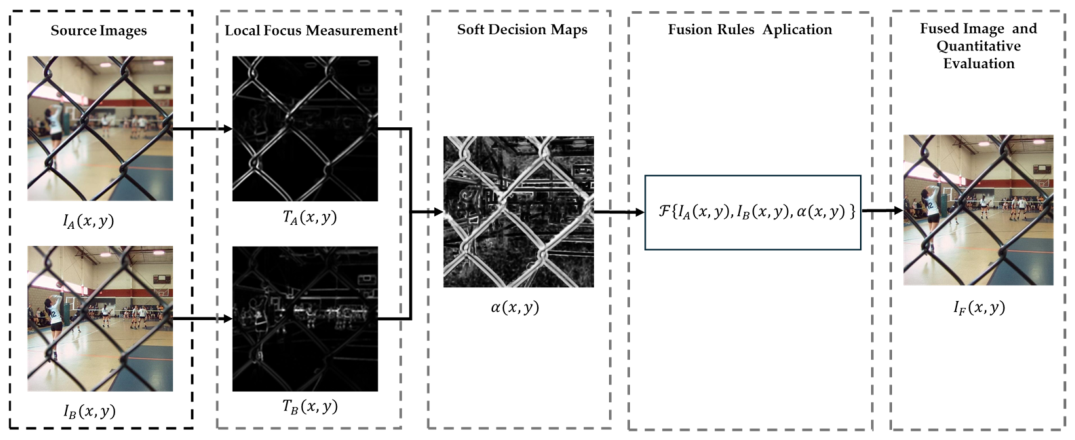
The proposed method is structured into four main stages: LFM computation, SDM construction, FR application, and quantitative evaluation. Figure 1 illustrates the overall workflow of the proposed method.

Given a pair of multi-focus input images $I_A(x,y)$ and $I_B(x,y)$, the focus measures $T_A(x,y)$ and $T_B(x,y)$ are first computed. Subsequently, a soft decision map $\alpha (x,y)$ is constructed, containing values within the interval $[0,1]$. Finally, the FR $F\{∎\}$ is applied to obtain the fused image $I_F(x,y)$, which is then evaluated using qualitative metrics.

2.1. Datasets

The proposed method is evaluated using two widely used datasets in the MFIF literature: Lytro (comprising 20 pairs of images captured at different focal planes) and MFI-WHU (consisting of 120 pairs of multi-focus images). In both cases, each image pair corresponds to the same scene with variations in the focused regions, enabling the evaluation of the algorithm's ability to properly integrate sharp areas from different source images.

In the case of the MFI-WHU dataset, where defocused regions are synthetically generated, a fully focused image (Ground Truth, GT) is also provided for each scene. This feature enables the use of reference-based metrics for a more accurate quantitative evaluation. In contrast, the Lytro dataset contains only multi-focus image pairs without GT, making it suitable for assessing the method's performance in non-reference scenarios, which are closer to real-world applications where a fully focused image is not available.

2.2. Local Focus Measure Estimation

To estimate the LFM in the source images, the classical Tenengrad focus measure [14] is employed. This is a low-computational-cost approach based on gradient magnitude, capable of estimating local sharpness. The measure relies on the premise that focused regions exhibit higher high-frequency content and, consequently, larger gradient magnitudes.

Thus, for a grayscale version of the source images $I(x,y)$, the horizontal and vertical gradient components, $G_X(x,y)$ and $G_Y(x,y)$, are computed along the $X$ and $Y$ directions, as defined in (1) and (2), respectively.

$$G_X\left(x,y\right)={\displaystyle \sum _{i=-1}^1}{\displaystyle \sum _{j=-1}^1}{K}_X\left(i,j\right)I\left(x+i,y+j\right)$$

(1)

$$G_Y\left(x,y\right)={\displaystyle \sum _{i=-1}^1}{\displaystyle \sum _{j=-1}^1}{K}_Y\left(i,j\right)I\left(x+i,y+j\right)$$

(2)

where $K_X$ and $K_Y$ represent the Sobel masks in the horizontal and vertical directions, respectively. Subsequently, the Tenengrad focus measure is applied to obtain the local gradient energy.

$$T\left(x,y\right)={\displaystyle \frac{1}{2w+1}}{\displaystyle \sum _{i=-w}^w}{\displaystyle \sum _{j=-w}^w}\left\{{G_X(x+i,y+j)}^2{{+G}_Y(x+i,y+j)}^2 \right\}$$

(3)

In (3), $w$ corresponds to the radius of the neighborhood centered at $(x,y)$. This procedure is applied independently to each source image $I_A(x,y)$ and $I_B(x,y)$ using $w=3$, which corresponds to a 7 × 7 neighborhood window, generating the energy maps $T_A (x,y)$ and $T_B (x,y)$, correspondingly, representing the LFM computed across each input image.

2.3. Soft Decision Map

A key aspect of the proposed methodology is the construction of a decision map that serves as a reference to determine the contribution of the LFM from each source image, thereby improving the performance of the FR. To this end, the approach is based on the premise that, in most classical MFIF methods, the FR relies on binary decision maps, where each pixel is entirely selected from the image with the higher focus measure. Although this approach is simple, as previously mentioned, it introduces abrupt transitions and may generate artifacts in regions where both images exhibit similar levels of focus. Therefore, to address this limitation, a non-binary decision map is adopted, namely, an SDM $\alpha (x,y)\in \left[\mathrm{0,1}\right]$, whose values are bounded within this interval. To construct it, a local-energy ratio is computed as:

$$\alpha \left(x,y\right)={\displaystyle \frac{T_A(x,y)}{T_A\left(x,y\right)+T_B\left(x,y\right)+\epsilon }}$$

(4)

where $T_A(x,y)$ and $T_B(x,y)$ denote the previously computed LFM for each input image, and $\epsilon ={1\times 10}^{-6}$ is a small positive constant introduced to avoid division by zero in regions where both LFM are close to zero. This value is selected to ensure numerical stability while having a negligible influence on the resulting SDM when relevant focus information is present.

From (4), it can be observed that $\alpha (x,y)\approx 1$ when $T_A(x,y)\gg T_B(x,y)$, i.e., when the LFM of image $I_A(x,y)$ is significantly higher than that of $I_B(x,y)$. Conversely, $\alpha (x,y)\approx 0$ when $T_A(x,y)\ll T_B(x,y)$. Finally, when both LFM are similar, $\alpha (x,y)\approx 0.5$. This SDM improves regions where the input images exhibit similar LFM, resulting in smoother transitions. This expression can be generalized to $N$ input images and their corresponding LFM $T_k(x,y)$. In this case, the SDM for the $k$-th image can be defined as:

$${\alpha }_k\left(x,y\right)={\displaystyle \frac{T_k(x,y)}{{\sum }_{i=1}^N{T}_i\left(x,y\right)+\epsilon }}$$

(5)

where $T_k(x,y)$ is the LFM computed from the source image $I_k(x,y)$, while the denominator corresponds to the sum of all LFM $T_i(x,y)$.

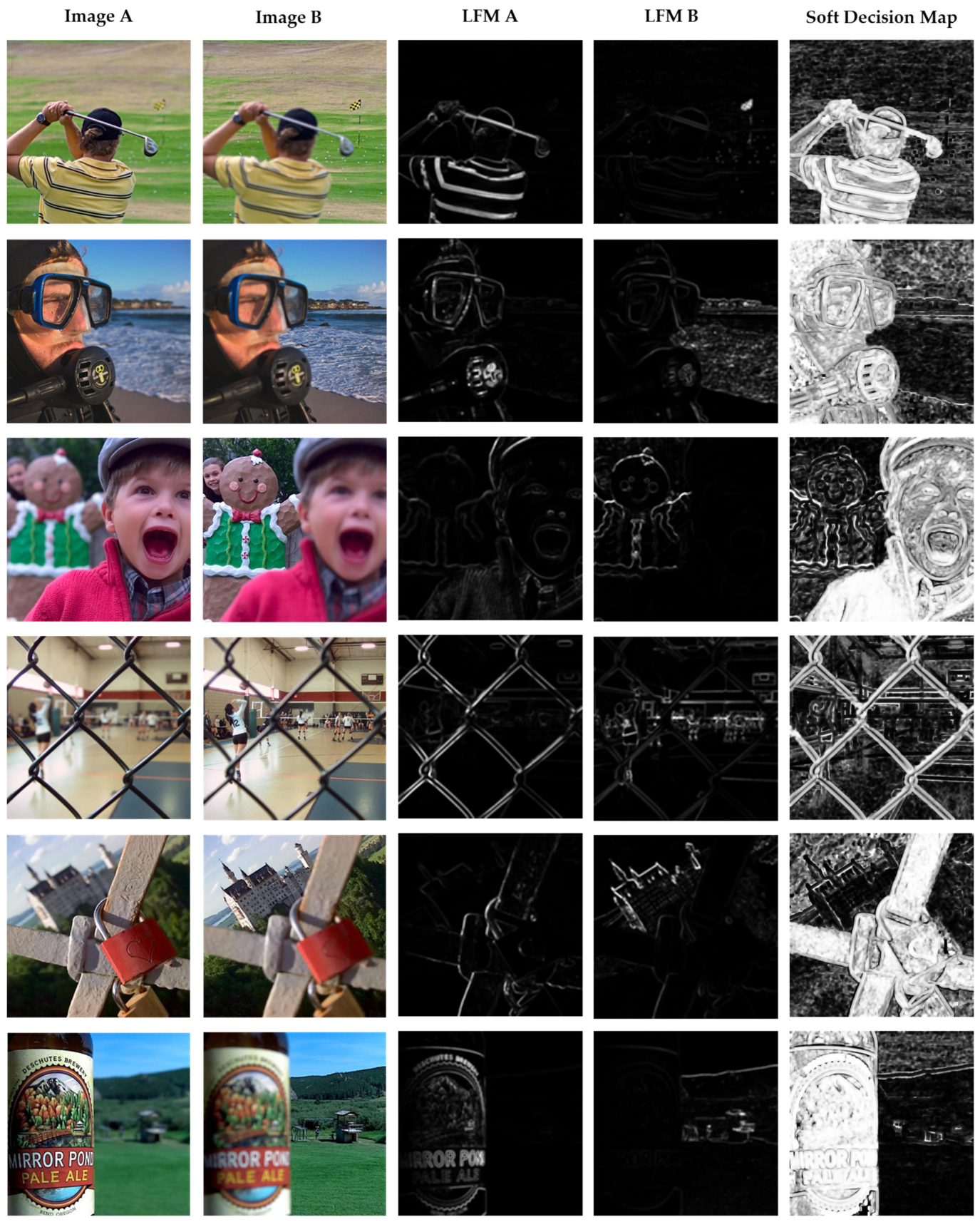
Figure 2 presents the numerical simulation of the proposed procedure. The first and second columns show the input images, Image A and Image B, respectively, whereas the third and fourth columns display the computation of the LFM for each image, LFM A and LFM B, respectively. Finally, the last column shows the SDM, where non-binary variations are represented in grayscale according to the previously computed local focus measures.

2.4. Fusion Rule

For the FR described in (6), two types of fusion operators $F\{∎\}$ are analyzed to study the quality of the fused image based on the two input images and the SDM. First, the well-known weighted linear (additive) fusion is employed; additionally, a fusion strategy based on a weighted geometric mean (multiplicative), is proposed, which, to the best of our knowledge, based on the reviewed literature, this FR has not been previously reported in the MFIF context considered in this work.

$$I_F\left(x,y\right)=\left\{I_A\left(x,y\right),I_B\left(x,y\right),\alpha (x,y)\right\}$$

(6)

2.4.1. Additive Fusion

The first FR corresponds to the well-known linear interpolation, widely used in the state of the art [26,27], and is defined as:

$$I_F\left(x,y\right)=\alpha \left(x,y\right)I_A\left(x,y\right)+\left(1-\alpha \left(x,y\right)\right)I_B(x,y)$$

(7)

From (7), it is clear that in regions where $\alpha =1$, the fused output image is determined by image $I_A$. Conversely, when $\alpha =0$, it is determined by image $I_B$. For intermediate values of $\alpha$, the fused image is obtained as a weighted average of both images. This expression can be generalized to $N$ input images as the weighted sum of all images:

$$I_F\left(x,y\right)={\displaystyle \sum _{k=1}^N}{I}_k\left(x,y\right){\alpha }_k; {\displaystyle \sum _{k=1}^N}{\alpha }_k=1$$

(8)

2.4.2. Multiplicative Fusion

To explore a nonlinear behavior, a FR based on a multiplicative-type weighted geometric mean is proposed, defined as:

$$I_F\left(x,y\right)={I_A\left(x,y\right)}^{\alpha \left(x,y\right)}{I_B(x,y)}^{\left(1-\alpha \left(x,y\right)\right)}$$

(9)

Before the fusion process, all source images are converted to a floating-point representation and normalized to the range $\left[0, 1\right]$. To ensure numerical stability, pixel values are constrained to the interval $\left[\epsilon , 1\right]$, where $\epsilon =1\times {10}^{-6}$, before applying the exponentiation. This avoids numerical issues associated with zero-valued pixels while preserving the behavior of the multiplicative FR. From (9), similarly to the linear FR, for $\alpha =1$ and $\alpha =0$, the fused image is determined by $I_A$ or $I_B$, respectively. For intermediate values of $\alpha$, the fused image corresponds to a weighted geometric mean of both images. This expression can be generalized to $N$ input images as the product of the weighted images:

$$I_F\left(x,y\right)={\displaystyle \prod _{k=1}^N}{I}_k{\left(x,y\right)}^{{\alpha }_k}; {\displaystyle \sum _{k=1}^N}{\alpha }_k=1$$

(10)

The proposed FR exhibits behavior analogous to the Cobb–Douglas production model, widely used in economics, where multiple factors contribute multiplicatively to the output through exponents that represent their influence [28]. This strategy tends to emphasize the input-image contributions in terms of their structural information, promoting greater discrimination between regions with similar focus levels while preserving fine details.

2.5. Quantitative Evaluation

To evaluate the performance of the proposed methodology, both reference-based and non-reference metrics are employed. Reference-based metrics assess the similarity between the fused image and a ground-truth reference image, whereas non-reference metrics evaluate the quality of the fused image based on perceptual properties.

Non-Reference Metrics

For both datasets, widely used non-reference metrics from the image fusion literature are employed:

• NMI (Normalized Mutual Information): measures the amount of information shared between the fused image and the source images [29]; and is defined as:

  $$NMI=2\left[{\displaystyle \frac{MI(I_F, I_A)}{H\left(I_F\right)+H\left(I_A\right)}}+{\displaystyle \frac{MI(I_F, I_B)}{H\left(I_F\right)+H\left(I_B\right)}}\right]$$

  (11)

  where $MI(I_F,I_A)$ and $MI(I_F,I_B)$ denote the mutual information between the fused image and each input image, respectively; and $H\left(I_F\right)$, $H\left(I_A\right)$, and $\mathrm{H}\left({\mathrm{I}}_{\mathrm{B}}\right)$, denote the marginal entropy of the fused image and each input image, respectively.
• Q_AB/F (Quality Assessment Based on Edge Information): evaluates the preservation of edges and gradient orientations in the fused image [30]; and is defined as:

  $$Q_{AB/F}={\displaystyle \frac{{\displaystyle {\sum }_{i=1}^N}{\displaystyle {\sum }_{j=1}^M}\left(Q_{AF}\left(i,j\right)w_A\left(i,j\right)+Q_{BF}\left(i,j\right)w_B(i,j)\right)}{{\displaystyle {\sum }_{i=1}^N}{\displaystyle {\sum }_{j=1}^M}\left(w_A\left(i,j\right)+w_B(i,j)\right)}}$$

  (12)

  where $Q_{AF}$ and $Q_{BF}$ indicate the loss of edge information transferred from the input images to the fused image of size $M\times N$. $w_A$ and $w_B$ are weights computed by applying an edge operator at each pixel $(i,j)$ in the input images.
• Q_CB (Chen–Blum Contrast Fusion Quality Index): quantifies the consistency of local contrast with respect to the source images [31]; and is defined as:

  $$Q_{CB}={\lambda }_A\left(i,j\right)Q_C^{AF}\left(i,j\right)+{\lambda }_B(i,j)Q_C^{BF}(i,j)$$

  (13)

  where $Q_C^{AF}$ and $Q_C^{BF}$ represent the preservation of local contrast between each source image and the fused image, whereas ${\lambda }_A$ and ${\lambda }_B$ are weighting factors associated with visually important regions or regions with the highest focus level within each input image.
• SF (Spatial Frequency): measures the overall SF of the image; higher values indicate greater high-frequency content and, consequently, a higher level of detail [32]; and is defined as:

  $$SF=\sqrt{{RF}^2+{CF}^2}$$

  (14)

  $$RF=\sqrt{{\displaystyle \frac{1}{MN}}{\displaystyle \sum _{i=0}^{M-1}}{\displaystyle \sum _{j=1}^{N-1}}{\left(I_F\left(i,j\right)-I_F\left(i,j-1\right)\right)}^2}$$

  (15)

  $$CF=\sqrt{{\displaystyle \frac{1}{MN}}{\displaystyle \sum _{i=1}^{M-1}}{\displaystyle \sum _{j=0}^{N-1}}{\left(I_F\left(i,j\right)-I_F\left(i-1,j\right)\right)}^2}$$

  (16)

  where $RF$ and $CF$ denote the row and column spatial frequencies of the fused image $I_F$ of size $M\times N$, respectively.

These metrics quantify the global and structural similarity between the fused image and the fully focused ground-truth reference image.

2.6. Computational-Cost Analysis

In addition to the quality assessment, the execution times corresponding to each stage of the proposed methodology are recorded. The total execution time of the algorithm is defined as the sum of the time required by the following stages: (a) LFM computation, (b) SDM construction, and (c) FR application.

3. Experimental Evaluation

In this section, the MFI-WHU dataset, consisting of 120 pairs of multi-focus images and their corresponding GT images, is used to evaluate the performance of the proposed method using the no-reference metrics NMI, QAB/F, QCB, and SF. Similarly, the Lytro dataset, which contains 20 pairs of multi-focus images, is employed to assess the performance of the proposed method using the same set of no-reference metrics. The obtained results are compared with those of eight representative state-of-the-art fusion algorithms: Multi-Focus Image Fusion based on Residual Removal (MFIF-RR) [33], Multimodal Medical Image Fusion based on Joint Bilateral Filter (MMIF-JBF) [34], Generative Adversarial Network for Multi-Focus Image Fusion (MFIF-GAN) [35], a General Unsupervised Image Fusion Network based on Memory Unit (MUFusion) [36], Small-Area-Aware Multi-Focus Image Fusion (SAMF) [37], Adaptive Region Division Multi-Focus Image Fusion (RDMF) [38], Bridging the Gap between Multi-Focus and Multi-Modal Image Fusion (MFIF-MMIF) [9], and Gradient-Based Multi-Focus Image Fusion (Gradient-MFIF) [39]. The baseline results for these state-of-the-art MFIF methods are retrieved from Li and Li (2025) [39], which provides a unified benchmark of the aforementioned methods evaluated on common public datasets using the same set of objective quality metrics. This benchmark enables a consistent and fair comparison with the proposed approach.

For the proposed method, a 7 × 7 neighborhood window is used for LFM computation and SDM construction. In addition, two FR are evaluated: the conventional Additive FR and the Multiplicative FR introduced in this work. The reported results correspond to the average values obtained across all image pairs in each dataset. Before the fusion process, all source images are converted to a floating-point representation and normalized to the range [0, 1]. Subsequently, for the computation of the LFM, the grayscale version of each previously normalized image is used. From these LFM, the SDM is generated. Finally, the proposed FR are applied to the three RGB channels of the source images. In all experiments, the images from the public MFI-WHU and Lytro datasets are processed while preserving their original spatial resolution, without resizing. Performance evaluation is carried out using NMI, SF, Q_AB/F, and Q_CB, following the corresponding formulations described in Section Non-Reference Metrics.

In addition to fusion quality, the computational cost of the proposed method is evaluated, measured in seconds, to assess its suitability for real-time applications. The experiments are conducted on a workstation running Pop!_OS 22.04 LTS (64-bit), equipped with an Intel Core i7-10750H processor (12 threads, up to 5.0 GHz) and 16 GB of RAM. All computations are performed exclusively on the Central Processing Unit (CPU).

3.1. Quantitative Comparison

Table 1. Performance comparison of state-of-the-art methods on the MFI-WHU dataset.

Method	NMI	QAB/F	QCB	SF
MFIF-RR	1.184	0.728	0.822	26.760
MMIF-BJF	1.038	0.723	0.778	26.696
MFIF-GAN	1.184	0.732	0.822	26.850
MUFusion	0.728	0.599	0.647	22.585
SAMF	1.188	0.726	0.820	26.667
RDMF	1.174	0.728	0.823	26.591
MFIF-MMIF	1.038	0.717	0.791	25.846
Gradient MFIF	1.185	0.733	0.825	26.783
Proposed (Additive Fusion)	0.949 ± 0.147	0.735 ± 0.014	0.907 ± 0.008	23.711 ± 8.633
Proposed (Multiplicative Fusion)	0.953 ± 0.146	0.734 ± 0.014	0.912 ± 0.008	23.886 ± 8.667

and

Table 2. Performance results on the Lytro dataset using non-reference metrics.

Method	NMI	QAB/F	QCB	SF
MFIF-RR	1.1261	0.7530	0.8018	19.4040
MMIF-BJF	0.8931	0.7140	0.6690	18.6682
MFIF-GAN	1.1313	0.7529	0.8005	19.4271
MUFusion	0.7983	0.6624	0.6770	18.9482
SAMF	1.1191	0.7511	0.7951	19.3820
RDMF	1.1221	0.7518	0.8010	19.3444
MFIF-MMIF	0.9329	0.7318	0.7338	18.5671
Gradient MFIF	1.1292	0.7531	0.8024	19.4308
Proposed (Additive Fusion)	0.974 ± 0.1267	0.756 ± 0.035	0.915 ± 0.02	18.00 ± 5.996
Proposed (Multiplicative Fusion)	0.982 ± 0.123	0.756 ± 0.035	0.924 ± 0.02	18.32 ± 6.139

present the quantitative comparison between the proposed method and eight representative methods from the literature, using non-reference metrics on the two evaluated datasets. It should be noted that the performance metrics reported in [39] for the MFI-WHU dataset do not include the reference-based measures PSNR (Peak Signal-to-Noise Ratio) and SSIM (Structural Similarity Index). To provide a more comprehensive evaluation of the proposed approach, these metrics are computed using the fully focused GT images available in the dataset. Specifically, PSNR quantifies the reconstruction error relative to the GT image, with higher values indicating lower distortion, whereas SSIM assesses structural similarity by jointly considering luminance, contrast, and local image structure, with values closer to 1 indicating greater similarity. The proposed method, in its additive FR and multiplicative FR variants, achieves PSNR values of 33.84 dB and 33.75 dB, respectively, while both variants obtain an SSIM value of 0.985. These results demonstrate that the fused images exhibit a high degree of fidelity and structural consistency with respect to the fully focused GT images.

Regarding the non-reference metrics in Table 1, the Multiplicative Fusion variant achieves a slightly higher NMI value than the Additive Fusion variant; however, its performance remains slightly below that of most state-of-the-art methods. On the other hand, for the $Q_{CB}$ and $Q_{AB/F}$ metrics, both fusion variants proposed in this work exhibit highly competitive performance, achieving values of up to $Q_{CB}=0.912$ and $Q_{AB/F}=0.735$. These results indicate effective preservation of local contrast, as well as superior retention of edge information and structural details in the fused images. In particular, the $Q_{CB}$ and $Q_{AB/F}$ values achieved by the proposed methods outperform those of the compared approaches, highlighting their ability to efficiently preserve visually relevant information throughout the fusion process. It is worth noting that both proposed variants obtain slightly lower SF values; however, since this metric measures high-frequency content without distinguishing between meaningful details and noise, these results suggest that the proposed method preserves relevant structures better while simultaneously reducing the amplification of unwanted noise components.

Table 2 presents the results obtained on the Lytro dataset using only non-reference metrics. Consistent with the results observed for the MFI-WHU dataset, the proposed variants achieves a slightly higher NMI values than the Additive Fusion variant; however, its performance remains slightly below that of most state-of-the-art methods. Regarding the $Q_{AB/F}$ and $Q_{CB}$ metrics, the proposed methods achieve the best results, reaching values of up to 0.756 and 0.924, respectively. These results demonstrate excellent edge preservation and high contrast quality in the fused images. On the other hand, the obtained SF values are slightly lower than those reported by some of the competing methods. However, as previously discussed, this metric does not distinguish between meaningful details and noise. Therefore, the results suggest that the proposed method favors the preservation of relevant structures while limiting noise amplification, ultimately contributing to improved visual quality in the fused images.

Based on the results obtained across both datasets, the proposed method demonstrates a more balanced performance compared with state-of-the-art approaches when all evaluation metrics are considered jointly. It particularly stands out in terms of Q_AB/F and Q_CB, indicating superior edge preservation and better local contrast consistency in the fused images. Moreover, it maintains competitive NMI, reflecting effective information retention and high structural fidelity. Overall, these results demonstrate that the proposed method provides a favorable balance among structural quality, information content, and perceptual image quality.

3.2. Qualitative Results

To visually compare the fusion results produced by the proposed method, Figure 3 and Figure 4 present the output obtained by using the two FR considered in this work on both datasets. Unlike the quantitative comparison, this section focuses exclusively on the proposed variants, as they achieve a competitive performance compared with the state-of-the-art methods according to the evaluated objective metrics.

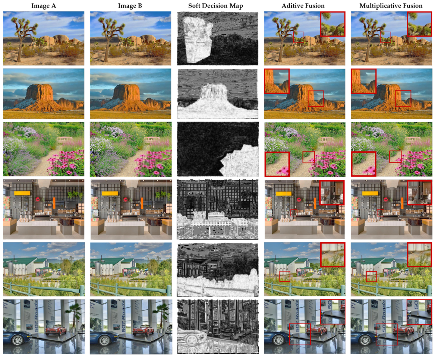
Figure 3 presents six image pairs from the MFI-WHU dataset, showing the source images (Image A and Image B), the SDM generated by the proposed methodology, and the fused images obtained using the Additive and Multiplicative FR. As can be observed, the SDM effectively identifies the regions with the highest local focus level in each image, thereby facilitating the fusion process. In the resulting fused images, the Additive FR produces smoother transitions between regions, helping to reduce the occurrence of visual artifacts. In contrast, the Multiplicative FR provides sharper edge and texture definition, enhancing the preservation of fine details in the fused image.

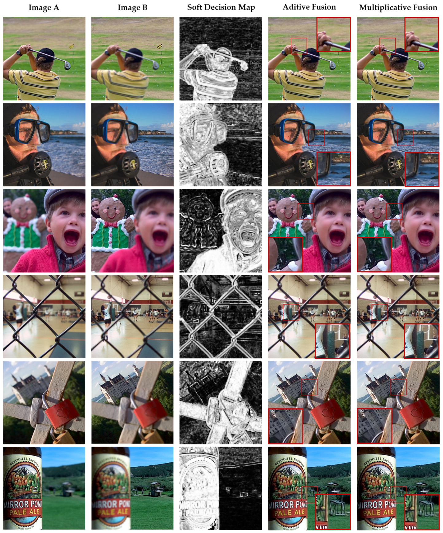
Figure 4 presents six image pairs from the Lytro dataset. Similar to the results observed on the MFI-WHU dataset, the Additive FR produces visually homogeneous images with smooth transitions between regions and without abrupt changes. In contrast, the Multiplicative FR stands out for its ability to preserve fine details and enhance the visual perception of the scene, particularly in regions with greater structural complexity and depth.

3.3. Computational Cost

In addition to the quality of the fused images, the computational cost of the proposed method is evaluated to assess its suitability for real-time applications. The algorithm is implemented in Python (Version 3.12.7) using standard numerical and image-processing libraries. Since the methodology relies primarily on local gradient operations and simple arithmetic computations, and simple algebraic operations, it does not require GPU acceleration, thereby maintaining low computational complexity and facilitating reproducibility across different hardware platforms.

Execution times are measured on an Intel Core i7-10750H CPU and correspond to the processing time per image pair. The reported values are presented as mean ± standard deviation over all image pairs in each dataset, namely 20 pairs for Lytro and 120 pairs for MFI-WHU. All images are processed at their original spatial resolution, without resizing. The timing measurements include the computation of the LFM, the generation of the SDM, and fusion-rule application. File input/output operations are excluded from the measurements, and all experiments are performed using CPU resources only.

Table 3. Average execution time using the Additive and Multiplicative FR on both datasets.

Method	MFI-WHU	Lytro
Proposed (Additive fusion)	0.007 ± 0.002 s	0.007 ± 0.0003 s
Proposed (Multiplicative fusion)	0.026 ± 0.008 s	0.027 ± 0.0007 s

presents the results of the computational cost analysis. The proposed method achieves low execution times in both datasets. In particular, the Additive Fusion variant requires approximately 0.007 s per image pair, whereas the Multiplicative Fusion variant requires approximately 0.026–0.027 s. This difference is attributed to the higher computational cost associated with the multiplicative and exponential operations involved in the Multiplicative Fusion Rule, compared with the weighted summation used in Additive Fusion.

Although a direct comparison of computational complexity with the considered state-of-the-art methods is not feasible, since most of them rely on deep learning techniques, multiscale transforms, image-domain transformations, and other computationally intensive processes, it is important to emphasize that the proposed method is composed of lightweight operations. As a result, it provides an efficient implementation with low execution times and modest computational requirements.

4. Discussion

The obtained results allow analyzing the proposed methodology's performance from three complementary perspectives: (i) fusion quality assessed through objective metrics, (ii) qualitative analysis focused on edge preservation, contrast, and information transfer, and (iii) computational cost. Taken together, the results demonstrate that the proposed method provides competitive performance regarding non-reference metrics when compared with state-of-the-art methodologies, considering the balance between fusion quality and computational efficiency. In particular, the high PSNR and SSIM values obtained with Additive FR and Multiplicative FR indicate that both methods effectively reconstruct fused images that are highly consistent with the fully focused reference images. Furthermore, it is worth noting that these metrics are not reported by the compared state-of-the-art methods, making it difficult to directly assess their accuracy with respect to a GT image.

When analyzing the no-reference metrics, the proposed method achieves a well-balanced performance across NMI, Q_AB/F, and Q_CB, improving information preservation, edge retention, and local contrast enhancement. Although the obtained NMI values are not the highest among the evaluated methods, they remain very close to those reported by approaches with significantly higher computational complexity. This suggests that the proposed method efficiently integrates the most relevant information from the source images while avoiding unnecessary redundancy in the fused result.

It is important to highlight the slightly lower values obtained for the SF metric. Although high SF values are often associated with a high level of detail, this metric does not differentiate between meaningful information and noise components. In this context, the results suggest that the proposed method avoids artificially enhancing high-frequency components, thereby promoting a more controlled fusion process. As a result, noise amplification is reduced while preserving the structures and details that are truly relevant to the scene.

The qualitative analysis reinforces the findings obtained from the quantitative metrics, revealing clear differences between the two proposed fusion strategies. Additive Fusion produces smoother and more homogeneous images, with gradual transitions between regions, thereby enhancing visual consistency and reducing the presence of artifacts. In contrast, Multiplicative Fusion, due to its nonlinear nature, emphasizes fine details and local contrast, resulting in improved edge and texture definition. These differences confirm that both approaches exhibit complementary characteristics. While Additive Fusion prioritizes smoothness and visual consistency, Multiplicative Fusion favors detail preservation and structural discrimination. Therefore, the most suitable strategy can be selected according to the specific requirements of the target application.

From a computational perspective, the proposed method demonstrates high efficiency, achieving very low execution times that make it suitable for real-time applications. The difference observed between the Additive and Multiplicative Fusion schemes is directly related to the complexity of the operations involved in each approach. Nevertheless, both variants maintain low processing times, confirming the feasibility of the proposed method for deployment in computationally constrained environments.

5. Conclusions

In this work, an MFIF method based on LFM and an SDM is proposed, incorporating two FR strategies: Additive Fusion and Multiplicative Fusion. Both variants are evaluated on the MFI-WHU and Lytro datasets using non-reference metrics, qualitative assessment, and computational cost analysis. The results show that the proposed method achieves competitive and well-balanced performance compared with state-of-the-art approaches, particularly in edge preservation (Q_AB/F) and contrast enhancement (Q_CB), while maintaining adequate shared information (NMI) and high structural fidelity (SSIM). Although the SF values are slightly lower, this suggests a controlled fusion process that preserves relevant structures without unnecessarily enhancing high-frequency components. The qualitative results show that the two fusion strategies have complementary behavior. Additive Fusion produces smoother and more visually homogeneous images, making it suitable when visual consistency is prioritized. In contrast, Multiplicative Fusion better preserves fine details and enhances local contrast, which is useful when structural definition is critical. From a computational perspective, the method achieves low execution times because it relies on simple local operations, making it suitable for real-time applications without specialized hardware. Overall, the proposed framework offers a favorable balance between fusion quality, structural preservation, perceptual quality, and computational efficiency. Future work will explore hybrid MFIF frameworks that integrate the proposed methodology with deep-learning techniques for feature extraction and decision-map refinement. These studies will include quantitative comparisons with representative methods, while maintaining computational efficiency as a key objective.